Johns Hopkins University, Dept. of Biostatistics Working Papers
4-12-2007
A BAYESIAN HIERARCHICAL FRAMEWORK
FOR SPATIAL MODELING OF f MRI DATA
F. DuBois Bowman
Department of Biostatistics, The Rollins School of Public Health, [email protected]
Brian S. Caffo
Department of Biostatistics, The Johns Hopkins Bloomberg School of Public Health
Susan Spear Bassett
Department of Psychiatry and Behavioral Sciences, Johns Hopkins Medical Institutions
Clinton Kilts
Department of Psychiatry and Behavioral Sciences, Emory University
Suggested Citation
Bowman, F. DuBois; Caffo, Brian S.; Spear Bassett, Susan; and Kilts, Clinton, "A BAYESIAN HIERARCHICAL FRAMEWORK FOR SPATIAL MODELING OF fMRI DATA" (April 2007).Johns Hopkins University, Dept. of Biostatistics Working Papers.Working Paper 139.
A Bayesian Hierarchical Framework for Spatial Modeling of
fMRI Data
F DuBois Bowman∗, Brian Caffo†, Susan Spear Bassett‡, Clinton Kilts§
April 12, 2007
Abstract
Functional neuroimaging techniques enable investigations into the neural basis of human cognition, emotions, and behaviors. In practice, applications of functional magnetic resonance imaging (fMRI) have provided novel insights into the neuropathophysiology of major psychi-atric, neurological, and substance abuse disorders, as well as into the neural responses to their treatments. Modern activation studies often compare localized task-induced changes in brain activity between experimental groups. One may also extend voxel-level analyses by simultane-ously considering the ensemble of voxels constituting an anatomically defined region of interest (ROI) or by considering means or quantiles of the ROI. In this work we present a Bayesian exten-sion of voxel-level analyses that offers several notable benefits. First, it combines whole-brain voxel-by-voxel modeling and ROI analyses within a unified framework. Secondly, an unstruc-tured variance/covariance for regional mean parameters allows for the study of inter-regional functional connectivity, provided enough subjects are available to allow for accurate estima-tion. Finally, an exchangeable correlation structure within regions allows for the consideration of intra-regional functional connectivity. We perform estimation for our model using Markov Chain Monte Carlo (MCMC) techniques implemented via Gibbs sampling which, despite the high throughput nature of the data, can be executed quickly (less than 30 minutes). We apply our Bayesian hierarchical model to two novel fMRI data sets: one considering inhibitory control ∗Department of Biostatistics, The Rollins School of Public Health
†Department of Biostatistics, Johns Hopkins Bloomberg School of Public Health ‡Department of Psychiatry and Behavioral Sciences, Johns Hopkins Medical Institutions §Department of Psychiatry and Behavioral Sciences, Emory University
in cocaine-dependent men and the second considering verbal memory in subjects at high risk for Alzheimer’s disease. The unifying hierarchical model presented in this manuscript is shown to enhance the interpretation content of these data sets.
Key words and phrases: functional imaging, image analysis, MCMC, medical imaging,
neuroimag-ing, regions of interest.
1 Introduction
Functional neuroimaging techniques enablein vivo investigations into the neural basis of human
cognition, emotions, and behaviors. In practice, applications of functional magnetic resonance imaging (fMRI) have provided insights into the pathogenesis and pathophysiology of major psy-chiatric, neurologic, and substance abuse disorders, as well as into the neural responses to their
treatments. We commonly employ fMRI to conductactivationstudies and studies offunctional
con-nectivity, depending on the research objectives. Activation studies generally seek to characterize
the magnitude and volume of neural responses to experimental tasks by detecting differences in patterns of brain activity between various experimental conditions, between different subgroups of subjects, and between two or more scanning sessions, e.g. before and after treatment. The objective of functional connectivity studies is to determine different areas of the brain that share similar temporal task-related (or resting-state) brain activity properties. Currently applied tech-niques consist of distinct statistical methodology for activation and functional connectivity studies. We develop a common statistical framework for activation and functional connectivity studies, and activation results from our approach account for prominent functional connections in the brain.
We develop a statistical modeling framework that builds on the two-stage approach commonly applied in activation studies for fMRI data. The conventional two-stage approach considers in-dividualized models at the first stage and population- or group-level models at the second stage (Worsley et al., 2002), both fitting separate models at each voxel. The voxel-by-voxel analyses employ estimation techniques that assume an improbable lack of correlation between voxel pairs. However, there is emerging recognition of the importance of modeling spatial correlations between voxels both for estimation and for statistical inferences. Some investigators attempt to capture
correlations between the measured brain activity in a given voxel with the activity in neighboring voxels. For example, Katanoda et al. (2002) address spatial correlations by incorporating the time series from neighboring (physically contiguous) voxels. Similarly, G¨ossl et al. (2001) and Woolrich et al. (2004a) consider correlations between neighboring voxels using a conditional autoregressive (CAR) model in a Bayesian framework, and specifically Woolrich et al. (2004a) model correlations as a function of the geometric mean of the number of neighboring voxels. Penny et al. (2005) present a Bayesian model that assumes spatially correlated prior distributions for the regression coefficients. They consider first-order neighbors (possibly extendable) in their spatial model and assume that the covariance matrix is known up to a multiplicative constant by defining a known spatial kernel matrix and by specifying a prior gamma distribution for the unknown constant.
Other authors extend spatial modeling beyond a localized neighborhood by simplifying the structure of the data. For example, Worsley et al. (1991) present a quadratic decay spatial cor-relation model for PET data from a selected number of anatomical regions, rather than voxels, significantly reducing the data and the dimensions of the correlation matrix. In a loosely related ap-plication, Albert and McShane (1995) present a generalized estimating equations (GEE) approach for spatially correlated binary data from a study of brain lesions, with a relatively small number
(e.g. 88) of spatial locations in each slice. Bowman (2007) considers data from a defined region
of interest and presents a spatio-temporal model that specifies spatial correlations based on a func-tionally defined distance metric. In this model, the magnitude of correlations decay as a function of decreasing similarity, rather than simply as a function of increasing physical distance, allowing the possibility of long range correlations due, for example, to white-matter axonal connections.
Bowman (2005) presents a whole-brain spatio-temporal model that partitions voxels into func-tionally related networks and applies a spatial simultaneous autoregressive model to capture intra-regional correlations between voxels. A key practical advantage of this approach is that it leads to fast estimation. Woolrich et al. (2004b) propose a Bayesian modeling framework for fMRI data allowing both separable and nonseparable spatio-temporal models. As an alternative to model-ing spatial correlations, one may indirectly address non-independence between voxels by initially smoothing the data, performing separate univariate analyses at each voxel, and then applying random field theory to determine statistical significance for the entire set of voxels, which makes
assumptions about spatial dependencies between voxels (Worsley et al., 1992; Worsley, 1994). The random field theory approach to hypothesis testing links voxel-wise statistics, generally by assuming a stationary or isotropic random field, but it does not directly estimate spatial covari-ances/correlations under a linear model. Holmes et al. (1996) outlines several issues with the random field approach, including low degrees of freedom to support the theory, noisy statistic images, a questionable assumption of constant error variance across an entire image, and initial spatial smoothing of the data.
The spatial modeling approaches of Katanoda et al. (2002), G¨ossl et al. (2001), and Woolrich et al. (2004a) provide local smoothing, but limiting spatial associations to a very restricted area (e.g. consisting of contiguous voxels) departs from our current knowledge regarding neurophys-iology including functional networks that are spatially disperse (e.g. the visual system). Broca’s area and Wernicke’s area are specific examples of two noncontiguous anatomical regions that may exhibit long range correlations, given their joint involvement in many language related tasks (Mat-sumoto et al., 2004). Bowman (2007) demonstrates that a relatively distant pair of voxels may exhibit high positive correlations, even when compared to a more proximal pair of voxels. Local spatial models disregard the possibility of such long-range correlations. Although the approach of Penny et al. (2005) is capable of extending the localized region, it makes an assumption of a known local spatial kernel, rather than estimating all of the variances and spatial covariances from the data.
Considering a coarsened data structure, such as the methods of Worsley et al. (1991) and Albert and McShane (1995), simplifies computations, but sacrifices the potential for localization using fMRI (or PET) data. Bowman (2005) frames a spatial model within a simplified data structure by modeling intra-regional correlations. While this method may incorporate long-range spatial correlations and provides inferences at a refined voxel level as well as broader regional levels, it suffers from the assumption that inter-region voxel pairs are uncorrelated. In contrast to the computationally efficient method of Bowman (2005), the approaches by Woolrich et al. (2004a), G¨ossl et al. (2001), and Bowman (2007) require extensive computations. Consequently, these methods are less practical due to the long computation times or are limited to small or moderate anatomic regions. For example, Bowman (2007) only considers analyses for regions of interest,
such as the cerebellum, and the method of Woolrich et al. (2004a) takes roughly 6 hours to analyze data from a single slice.
In this paper, we develop a Bayesian hierarchical statistical model for spatially correlated neu-roimaging data. Specifically, we develop a new spatial model for making inferences regarding task-related changes in brain activity, which identifies and accounts for prominent functional con-nections in the brain. Hierarchical models are general tools for estimating and making inferences about quantities that can be conceptualized through a multi-level process. The Bayesian hierarchi-cal approach provides a viable alternative to classihierarchi-cal statistihierarchi-cal methods for fitting complex models because it divides the parameters across different stages of the model that can be estimated using Markov chain Monte Carlo (MCMC) methods. Bayesian methods offer inferential advantages by providing samples from the joint posterior probability distribution for all of the model parame-ters, rather than p-values, providing greater flexibility in the inferences that may be drawn from a functional neuroimaging study.
Below, we discuss the proposed Bayesian hierarchical model, estimation procedures, and ap-plications of our model to experimental data from two fMRI studies. The main advantages that our proposed spatial model yields are that it: 1) provides a novel approach to uncover prominent functional connections between remote voxels, 2) often provides higher accuracy and increased sta-tistical power for inferences regarding task-related changes in brain activity by adjusting for spatial associations in the data, 3) extends the modeling assumptions underlying previously applied meth-ods from the limited amount of research in this area, and 4) establishes a unified framework that yields results for voxel-specific inferences, regional or VOI inferences, and functional connectivity.
2 Experimental fMRI data
2.1 Inhibitory control in cocaine-dependent men
Impairments in the ability to exert inhibitory control over drug-related behaviors, in spite of ad-verse consequences, represents a common characteristic of drug addictions (Kalivas and Volkow, 2005). These inhibitory control deficits exhibited by cocaine addicts can be modeled using response inhibition tasks outside of a drug seeking context. We consider an fMRI study that evaluates the
impact of cocaine addiction and treatment-related cocaine abstinence on neural representations of motor inhibition tasks targeting prepotent response inhibition.
Data are available for15cocaine-dependent men who have both pre- and post-treatment scans,
with the follow-up scans occurring roughly 24 days following the initial image acquisitions and
after completion of an intensive outpatient behavioral therapy program without relapse. Baseline
and follow-up scans are also available for 17 control subjects, matched to the clinical sample on
age, race, gender, handedness, education, and early life adversity. Within each session or treatment period, the data consist of serial fMRI scans on each person. Subjects received information about the procedures and risks of the study and provided written consent to participate in the study protocol approved by an Institutional Review Board.
Targeting inhibitory control processes, we consider scans corresponding to a Stop-signal task, designed to evaluate the ability to cancel a prepotent motor response (Aron and Poldrack, 2006). The task involves repeated presentations of visual Go stimuli (uppercase alphabetical letters), ap-pearing for 500 milliseconds with an inter-stimulus interval of2.3sec. Subjects execute the speeded Go response by pressing a button as quickly as possible. A Stop signal, an auditory tone (at1,000
Hz), lasting 500 milliseconds, occurs at random in16%of the trials. The presentation of the Stop
signal following the Go stimulus is an indicator to the subject to attempt to refrain from executing the Go response.
2.2 Alzheimer’s disease
Alzheimer’s disease is a debilitating degenerative disorder impacting millions of older adults in the United States alone (Brookmeyer et al., 1998). Currently there is no known cure, or effective treatments, for Alzheimer’s disease. Since pathologic changes occur before the onset of clinical symptoms, pre-clinical differences in neurological function between eventual Alzheimer’s cases and controls are of fundamental interest to early detection and intervention strategies. This observation is emphasized by the fact that the available treatments have greater clinical benefit the earlier they are introduced (see Tariot and Federoff, 2003, for example).
Bassett et al. (2006) demonstrated that fMRI activation patterns differ between subjects at high risk for Alzheimer’s disease and group-matched controls in an auditory word-pair-associate
task. This task, developed by Bookheimer et al. (2000), was chosen for its role as a processing demand for the medial temporal lobe (MTL), as the MTL is often indicated as an early site of neuropathological changes associated with Alzheimer’s disease . The auditory task consists of a memory “encode” phase, whereby subjects are presented unrelated word pairs in a block and a “recall” block, where subjects are asked to recall the second word of the pair when presented with the first. The paradigm consisted of two six minute sessions, each consisting of seven unique word-pairs.
Subjects were defined as at-risk for Alzheimer’s disease by having an autopsy confirmed affected parent and at least one additional clinically diagnosed first degree relative. Both at-risk and control
subjects were over50 years of age and free of memory impairments at the time of the study. All
subjects provided written consent and the study was approved by the Johns Hopkins Institutional Review board. The at-risk and control groups did not statistically differ on any key covariates.
However, there was some degree of asymmetry in terms of the number of APOE²4alleles, which
are a known marker for Alzheimer’s disease, and gender, with a higher percentage of females in the at-risk group.
Using this paradigm and sample, Bassett et al. (2006) found changes in neural activation be-tween the at-risk patients and the controls in the temporal lobe, including the frontal gyrii and right hippocampus. In this manuscript, we analyze a followup study on the same group of individ-uals using the same experimental paradigm. We focus only on comparison of the encode blocks to resting state. Notably, this study included nearly100subjects in each group, and limited the image acquisition to a small axial volume surrounding the MTL. As such, the study offers unique data for investigating functional connectivity between regions of interest.
3 A hierarchical model for functional neuroimaging data
We formulate a model that builds on the conventional two-stage modeling approach for fMRI data that emulates a random effects analysis. Our model captures temporal correlations via the random effects structure and by addressing serial dependencies between each subject’s repeated measure-ments, e.g. assuming an autoregressive-type model (Worsley et al., 2002). We extend the
con-ventional approach by fitting a spatial Bayesian hierarchical model at the second stage, where we capture correlations between voxels within defined neuroanatomical structures as well as between different anatomical regions. Incorporating spatial correlations into our statistical model allows us to quantify and make inferences about functional connections between intra-regional voxels and between defined anatomical nodes (regions).
3.1 Stage I: general linear model with serially correlated errors
In light of our two fMRI data examples examining response inhibition among cocaine-dependent men and verbal memory for subjects at-risk for Alzheimer’s disease, we present the Stage I model initially for an fMRI study. However, the general framework that we present is also applicable to PET regional cerebral blood flow (rCBF) studies, and one may consider a range of substantive applications that seek to identify localized regions of significant task-related (or between-group) changes in measured brain activity. The first-stage of our approach resembles a general linear model (GLM) for each individual’s vector of serial responses at the voxel level (Friston et al., 1995). To set notation, let i = 1, . . . , Kj index subjects, s = 1, . . . , S represent scans, andv = 1, . . . , V index voxels. We arrange the serial fMRI blood oxygenation-level dependent (BOLD) responses for subject i, measured at voxel v, in the S ×1 vector Yi(v). The S×q design matrix Xiv includes
independent variables of interests such as experimental conditions, and Hiv contains covariates
that are not of substantive interest, e.g. including a high-pass filtering matrix used to remove unwanted low-frequency trends from the data. For fMRI analyses, we convolve the design matrix with a prespecified hemodynamic response function.
We specify the first-stage model as follows:
Yi(v) =Xivβi(v) +Hivνi(v) +²i(v), (1) whereβi(v) ={βi1(v), . . . , βiq(v)}0 andβij(v)is the effect corresponding to stimulusj (for subject
i),νi(v)includes parameters associated withHiv, and the mean-zero vectors of random errors²i(v) are independent and follow a multivariate normal distribution with varianceVar{²i(v)}=τv2I. To make the variance model assumption tenable, one may apply a pre-whitening transformation, e.g. based on a first-order autoregressive model, to address serial correlations between multiple scans.
3.2 Stage II: spatial Bayesian hierarchical model
We consider an anatomical parcellation of the brain consisting of g = 1, . . . , G regions, where we
may setGas high as116(Tzourio-Mazoyer et al., 2002). Alternative anatomical parcellations are
also available, for instance, one based on defined Brodmann regions (Garey, 1994). Generally, we expect a fair degree of similarity of the fMRI time courses for voxels within a region. For regiong,
which containsVg voxels, we denote the individualized Stage I estimate of the mean fMRI BOLD
response vector associated with stimulusjbyβigj ={βigj(1), . . . , βigj(Vg)}0. These estimates result from applying a Stage I model analogous to that specified in Equation 1, with effects in the design matrices suitably defined to correspond to the experimental tasks. We also modify our earlier notation here by collecting localized effects from all voxels in regionginto a single vector . Stage two of our analysis proposes a Bayesian hierarchical model that accounts for spatial correlations between intra-regional voxels and also between regions. In particular, our model has the following hierarchical structure:
βigj|µgj, αigj, σgj−2 ∼ Normal(µgj+1αigj, σgj2 I)
µgj |λ2gj ∼ Normal(µ0gj, λ2gjI) σgj2 |Γj ∼ Gamma(a0, b0) (2) αij |Γj ∼ Normal(0,Γj) λ−gj2 ∼ Gamma(c0, d0) Γ−j1 ∼ Wishart©(h0H0j)−1, h0 ª
whereµgj = (µgj(1), . . . , µgj(Vg))0 andαij = (αi1j, . . . , αiGj)0.
The first level of our hierarchical model specifies a multivariate normal likelihood function for
the response vectors, βigj , containing each subject’s mean BOLD activity from the experimental
tasks of interest (from Stage I). For each voxel,v= 1, . . . , Vg, the subject-specific quantitiesβigj(v) are assumed to vary randomly about a mean consisting of both a population-level mean parameter
µgj(v)and an individualized (random effect) componentαigj. Given the random effects parameter,
αigj, the covariance matrix ofβigj is given byσ2
gjI. Our model yields a conditional independence
mediated by the random effects parameters.
At the next level, the model expresses a prior belief that each voxel’s population mean, (for the
jth effect), arises from a normal distribution with a mean given by the overall region mean, i.e.
µ0gj(v) = µ0gj, for all voxels v = 1, . . . , V, plus mean-zero random error with variance λ2gj. The data will help to inform this prior assumption, but it seems to represent a reasonable starting point to assume that voxels within anatomically-defined regions exhibit task-related activity that deviates around an overall mean for that region. At the final level, our hierarchical model captures potential
functional connections between anatomical brain regions through the covariance matrix Γj. We
provide additional details regarding functional connectivity below in Section 3.3.
In addition to voxel-specific quantities, interest may also lie in regional parameters that pool a collection of voxels in a regionRg. From our model, it is natural to define regional parameters such as the mean regional activation: θgj =
P
v∈Rgµgj(v)/Vg. Another candidate would consider the
upper percentiles of regional activation. We can easily estimate these regional parameters using samples from the joint posterior distribution for all of our model parameters, taking into account the potential correlations between voxel-specific parameters from the region. The first level of the hierarchical model in 2 can be conceived from the following linear model formulation
βigj |µgj=µgj+1αigj+²igj, (3) where²igj ∼Normal(0, σgj2 I). Note that conditional on µgj,βigj has an exchangeable covariance structure, based on this model expression. Specifically,
Var(βigj |µgj) =γgg(j)J+σ2gjI,
whereγgg(j)isgth diagonal element fromΓj, representing the regional variance. The exchangeable model builds in (equal) correlations between all pairs of voxels within a defined anatomical region.
3.3 Functional connectivity
Our Bayesian hierarchical model (2) allows us to capture information regarding the functional connectivity both within a defined anatomical structure and between brain regions. Friston et al. (1993) describes functional connectivity as the correlations between remote neurophysiological
events. There has been considerable methodological developments for quantifying functional con-nectivity, including seed-based approaches (Hampson et al., 2002) that compute correlations be-tween a selected voxel (seed) and other voxels within the brain. Also, Patel et al. (2006a) and Patel et al. (2006b) develop a Bayesian modeling approach that quantifies functional connectivity as well as hierarchical relationships between functionally connected voxels, referred to as ascendancy.
Our model captures the functional connectivity between voxels within a defined anatomical region as well as inter-regional functional connectivity. A measure of the strength of the intra-regional functional connectivity is given by
ρgj= γ
(j)
gg
γgg(j)+σgj2
. (4)
Thus, ρgj reflects the coherence or the similarity in neural activity between voxels within a given anatomical structure and may vary for different effects, e.g. for patients and controls and for baseline versus post-treatment measurement occasions. One may structure the model to address intra-regional correlations within the same hemisphere or employ an extended model to addition-ally capture bilateral intra-regional correlations between voxels in separate hemispheres, e.g. the right and left amygdala.
Another component of the functional connectivity is that which occurs between anatomical regions, captured in our framework by modelingαij = (αi1j, . . . , αiGj)0as
αij |Γj ∼N(0,Γj)
We specify a Wishart prior forΓ−j1, allowing a flexible unstructured covariance matrix for theαij. The multivariate structure enables us to compute the inter-regional functional connectivity matrix (with respect to stimulusj) by
Rj ={Diag(Γj)}−1/2Γj{Diag(Γj)}−1/2, (5) where the(g1, g2)element inRjrepresents the functional connectivity between anatomical regions
3.4 Prior specifications
To effect our Bayesian hierarchical model, we seta0 = 0.1, b0 = 0.005,c0 = 0.1,d0 = 0.01, and
h0 = G. These values were evaluated to ensure that they resulted in a diffuse enough prior so
that results were governed by the observed data. The selection for h0 establishes a diffuse prior
for the covariance matrix, without raising concerns about an improper posterior distribution. We empirically specifyµ0gjby calculating the global mean across all subjects and intra-regional voxels.
For the inverse-Wishart prior, the degrees of freedom must satisfy h0 ≥ G to yield a proper
prior distribution. The spatial prior forαij becomes non-informative ash0approaches0(West and
Harrison, 1989), so we seth0=Gto reflect the most diffuse prior that our data can support, while
employing a proper prior distribution. A seemingly natural choice forH0j is a point estimate ofΓj. We use the sample covariance matrix corresponding to thejth effect to obtainH0j, calculated from
the subject- and effect-specific mean activity levels in each of the anatomical regions. Note that according to our model, the use of the sample covariance matrix provides a conservative estimate of the true variation as follows. Given our hierarchical model, the variance-covariance matrix of β¯ij = ( ¯βi1j, . . . ,β¯iGj)0, where β¯igj = V1g
PVg
v=1βigj(v), has additive contributions fromΓj and
diag(σ12j/V1, . . . , σGj2 /VG). However, we specify a prior based on a matrixH0j that subsumes both components of variation. We favor this use of a conservative point estimate, to safeguard against under-estimating the variability. In addition to specifying a diffuse prior and using a conservative estimate, we examine the sensitivity of our results to the sample covariance matrix by artificially reducing the correlations (covariances) using
H∗0j = (1−ω)H0j+ω{diag(H0j)}.
where 0 ≤ ω ≤ 1. To avoid introducing prior information that does not seem physiologically
plausible and that is not supported by the data, we consider small to moderate departures from the sample covariance matrix in our sensitivity analyses. For example, we considerω ∈ [0,0.25], reflecting up to a25%decrease in the correlation estimates produced by our data.
4 Estimation and posterior inference
We implement MCMC methods for estimation using Gibbs sampling. Applying MCMC methods in our context is complicated by the massive amount of data, the vast number of spatial locations, and the large number of parameters. While our model maps well to characteristics of functional neu-roimaging data and is neurophysiologically plausible, the conjugate model specification facilitates estimation by providing substantial reductions in computing time and memory.
We draw simulations from the joint posterior distribution by applying Gibbs sampler to the associated full conditional distributions. To simplify our presentation of the full conditional dis-tributions, let D−j1 = diag
³ V1σ1−j2, . . . , VGσGj−2 ´ , β¯gj = K1 j PKj v=1βigj, µ¯ = (¯µ1, . . . ,µ¯Gj)0, with ¯ µgj = V1g PVg v=1µgj(v), anduigj = ¡ βigj−µgj−1αigj ¢0¡ βigj−µgj−1αigj ¢
. The full conditionals are given by the following:
µgj ∼ Normal h Ωgj n λgj−2µ0gj+Kjσgj−2(¯βgj−1α¯gj) o ,Ωgj i σgj−2 ∼ Gamma a0+KjVg/2, 1 b0 + 1 2 Kj X i=1 uigj −1 αij ∼ Normal h Ψj n D−j1(¯βij −µ¯j) o ,Ψj i (6) λ−gj2 ∼ Gamma ( c0+Vg/2, µ 1 d0 + (µgj−µ0gj)0(µ gj−µ0gj) 2 ¶−1) Γ−j1 ∼ Wishart h0H0+ Kj X i=1 αijα0ij −1 , h0+Kj , whereΩgj = ³ λ−gj2+Kjσgj−2 ´−1 IandΨj = ³ Γ−j1+D−j1 ´−1 .
A key advantage of our Bayesian modeling framework, relative to prior approaches employing classical statistical methods, is that we obtain samples from the joint posterior distribution for all of the model parameters. A related advantage is that we can easily estimate functions of the model parameters using the posterior samples. Obtaining posterior samples for all parameters and relevant functions of the model parameters facilitates inferences by allowing us to formulate associated probability statements and to compute MCMC-based credible intervals, giving a specified probability that the parameter of interest lies in a particular interval. In addition to the parameters in model (2), we will estimate ρg to quantify intra-regional functional connectivity, Rj for
inter-regional connectivity, and θgj for regional-level effects, e.g. comparing pre- and post-treatment brain activity levels in specified anatomical regions.
5 Results
We apply our Bayesian hierarchical model to both the fMRI study of inhibitory control in cocaine-dependent men as well as to the auditory memory encoding and retrieval study of individuals who are at high risk for developing Alzheimer’s disease.
5.1 Voxel-level activations
Cocaine dependence data
Our analysis provides voxel-specific probabilities of any event that is definable as a function of the model parameters, providing a flexible framework to make inferences pertaining to a range of study objectives. We focus on inferences about neural processing alterations related to inhibitory control for cocaine-dependent men before and after intensive behavioral therapy for their addic-tion. To adjust for learning (or other) effects associated with repeated scanning at baseline and at the follow-up period, we quantify treatment-emergent changes in measured brain activity in the cocaine addicts relative to the corresponding alterations in the healthy control subjects. In sum-marizing the results from our analysis of the inhibitory control data, we quantify treatment-related changes in brain activity as the post-treatment quantity of interest (e.g. group average within a voxel or within a region) minus the pre-treatment quantity. Similarly, we quantify changes for the control subjects as follow-up estimates minus the baseline estimates.
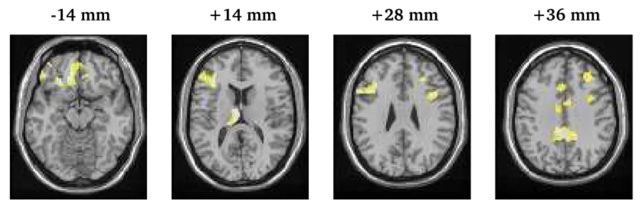
Figure 1 displays axial slices showing voxels exhibiting treatment-emergent inhibitory control-related changes in neural processing for the cocaine-dependent men that exceed the corresponding changes in the controls. The highlighted voxels have posterior probabilities exceeding 0.70 and include the medial orbital frontal cortex (BA 11), the left thalamus and left middle frontal gyrus (BA 46), the left and right middle frontal gyrus (BA 9), and the cingulate gyrus (BA 31, 32). The voxel-specific effects of treatment indicate the recruitment of thalamo-cortical pathways in attaining the relapse prevention goals of behavioral therapies. Functional inferences include the involvement of
-14 mm +14 mm +28 mm +36 mm
Figure 1: Maps of voxel-specific treatment-emergent activations for the cocaine-dependent subjects, adjusted for the corresponding baseline-to-follow-up changes in the control subjects. The maps portray voxel-specific posterior probabilities, exceeding0.70, of increased activity from baseline to the post-treatment period for the cocaine addicts, relative to (minus) the corresponding difference in the control subjects. The axial slices are at various distances (in millimeters (mm)) from the anterior-posterior commissural plane. The activations include the medial orbital frontal cortex (BA
11) [at−14mm], the left middle frontal gyrus (BA 46) and left thalamus [at+14mm], bilaterally
in the middle frontal gyrus (BA 9) [at+28mm], and along the cingulate gyrus (BA 31, 32), with
the posterior cingulate activation appearing most spatially extensive [at+36].
alterations in drug valuation and in the mental representation of drug contingencies, facilitation of regulatory control of responses to drug incentives, and the engagement of cognitive control processes related to response conflict monitoring drug availability.
Alzheimer’s disease data
The Alzheimer’s disease data showed no significant areas of voxel-level activation differences be-tween groups. Specifically, in no regions did at-risk subjects present evidence of significantly higher or lower activation than controls. The areas that survived thresholds were diffuse and not localized, which mirrors results found using standard voxel-level techniques. This may in part be due to the finer decomposition of imaging area into small regions of interest used in this analysis. As shown below, there was more support for the association of Alzheimer’s risk with alterations in regional activations and differences in connectivity.
5.2 Regional activations and functional connectivity
In addition to voxel-level inferences, our model provides a framework for investigating (de)activations at a regional level. Regional-level analyses have the advantage that they may pool strength from voxels across the entire region to reveal task-induced alterations in neural processing, even when the voxel-specific analyses do not reveal such changes. However, it is important to note that, de-pending on the number of activated voxels in a region and the magnitudes of these activations, one may not detect regional increases (decreases) in activity, despite having voxels within the region that show elevated (decreased) activity.
Cocaine dependence data
We evaluate regional treatment-related differences in the neural response to the inhibitory control task by computing mean estimates of the post-treatment period minus the pre-treatment period for the cocaine-dependent subjects, relative to the corresponding estimate in the control subjects. Specifically, we obtain probabilities that the treatment response in the cocaine addicts exceeds the (learning) response in the control group, and similarly we quantify the likelihood that the learning response in the controls exceeds the treatment-emergent response for the addicts.
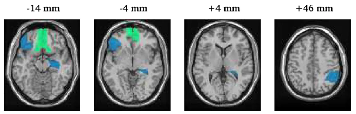
Figure 2 displays regions for which the posterior probabilities of treatment-related brain activity changes in the cocaine-dependent subjects are greater than (green) and less than (blue) than the changes in the healthy control subjects. The data provide evidence of treatment-related increases in inhibitory control-related activity in the medial orbital frontal cortex and the gyrus rectus, with posterior probabilities of0.85and0.94, respectively, estimated from the posterior distribution sam-ples. Examining the posterior mean estimates for the baseline to follow-up changes in brain activity separately for each group, we observe that the cocaine-dependent subjects exhibit an increase in activity in the medial orbital frontal cortex following treatment, whereas the control subjects show little change. The cocaine addicts also reveal large increases in activity following treatment in the gyrus rectus (0.79) compared to a slight increase in the controls (0.02). Our findings indicate that there is an estimated 85% chance that the change in neural functioning in the medial orbital frontal cortex from pre- to post-treatment exceeds the corresponding change in the control subjects, and
similarly there is an estimated94%chance that the treatment response in the gyrus rectus outpaces the learning response in the controls.
Our analysis also determines that the right inferior parietal cortex (posterior probability (pp)=0.89), the right hippocampus (pp=0.95), and the left inferior orbital frontal cortex (pp=0.95) all show greater baseline to follow-up changes in neural processing for the controls than pre- to post-treatment changes in the cocaine addicts. Both the cocaine addicts and the healthy controls show decreased activity in the right inferior parietal cortex at follow-up, on average, so one may view our results as indicating an89%chance that the decrease in the cocaine addicts is more extensive than the decrease in the controls. In the right hippocampus and in the left lateral orbital frontal cortex, the cocaine addicts demonstrate a decrease in activity following treatment, while the controls
re-veal increased activity. Therefore, our results indicate an estimated 95%chance that the baseline
to follow-up change in the regional mean BOLD response is greater in the controls than it is in the cocaine-dependent subjects. The results of the region-level analysis suggests the engagement of behavioral regulatory functions related to treatment-emergent activation of the ventromedial pre-frontal cortex and the lesser demand for the attentional, habit suppression and memory retrieval processes necessary to foregoing cocaine use in early abstinence states.
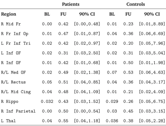
Our model yields estimates of the within-region correlations, based on the posterior means of
ρgj, giving a measure of regional coherence or intra-regional functional connectivity (see Table 1). We obtain separate estimates of the regional coherence for the cocaine addicts before and after treatment as well as for the control subjects at baseline and at follow-up. Both groups of subjects exhibit more synchronized intra-regional neural processing during the follow-up session relative to baseline, revealed by the increases in intra-regional correlations for each anatomical region. The cocaine addicts show a fair degree of coherence following treatment between voxels comprising the left thalamus (0.55), the right inferior parietal lobule (0.50), the gyrus rectus (0.51), and the medial orbital frontal cortex (0.49). The control subjects exhibit the strongest intra-regional correlations at the follow-up assessment in the medial (0.53) and right lateral (0.50) portions of the orbital frontal cortex.
We also evaluate whether the data provide evidence of more synchronous intra-regional neu-ral functioning at follow-up relative to baseline by considering the ratio of the pre-treatment (or
-14 mm -4 mm +4 mm +46 mm
Figure 2: Map of regional treatment-emergent activations (green) and deactivations (blue) for the cocaine-dependent subjects, adjusted for the corresponding baseline-to-follow-up changes in the control subjects. The axial slices portray regional (de)activations at various distances (in millime-ters) from the anterior/posterior commissural plane. All regions displayed have posterior probabil-ities of (de)activation exceeding0.80. The deactivations include the right inferior parietal cortex
(at+46mm), the right hippocampus (at−4and+4mm), and the left lateral orbital frontal cortex
(at−4 and−14 mm). The maps reveal evidence for activation in the right and left medial orbital
frontal cortex (at−4and−14mm) as well as the right and left gyrus rectus (at−14mm).
baseline) correlation to the post-treatment (or follow-up) correlation for each region, sayρg1/ρg2
(see Table 1). A value of this ratio falling below one indicates greater intra-regional coherence at follow-up, relative to baseline. The strongest evidence for more synchronous intra-regional neu-ral functioning at the follow-up session exists for the cocaine addicts, with the upper bounds of
the MCMC-based 90% credible intervals for ρ1/ρ2 falling below one for the right middle frontal
gyrus, the right pars operculum of the inferior frontal cortex, the pars triangularis of the left infe-rior frontal cortex, the right lateral orbital frontal cortex, the gyrus rectus, and the right infeinfe-rior parietal cortex, while all of the 90% credible intervals for the controls overlap one. These results suggest that a further description of treatment-related cocaine abstinence is the greater coherence of neural information processing in frontal and parietal brain regions involved in response inhibi-tion.
Patients Controls Region BL FU 90% CI BL FU 90% CI R Mid Fr 0.00 0.42 [0.00,0.48] 0.01 0.23 [0.01,8.89] R Fr Inf Op 0.01 0.47 [0.01,0.87] 0.04 0.36 [0.06,6.69] L Fr Inf Tri 0.02 0.42 [0.02,0.97] 0.02 0.20 [0.05,7.96] L Inf OF 0.02 0.31 [0.03,2.50] 0.02 0.31 [0.03,5.04] R Inf OF 0.01 0.42 [0.01,0.68] 0.01 0.50 [0.01,1.98] R/L Med OF 0.02 0.49 [0.02,1.38] 0.07 0.53 [0.06,4.63] R/L Rectus 0.05 0.51 [0.04,0.85] 0.04 0.36 [0.04,3.17] R/L Mid Cing 0.04 0.48 [0.04,1.09] 0.01 0.21 [0.02,4.09] R Hippo 0.032 0.43 [0.03,1.52] 0.029 0.26 [0.05,6.75] R Inf Parietal 0.00 0.50 [0.00,0.54] 0.03 0.45 [0.03,3.15] L Thal 0.04 0.55 [0.04,1.18] 0.036 0.38 [0.05,2.28]
Table 1: Posterior median estimates of the intra-regional correlations (functional connectivity) for selected anatomically-defined brain regions. Separate estimates appear for patients and
con-trols as well as for baseline and follow-up scanning sessions. The 90% credible intervals
corre-spond to the ratio of the baseline regional correlation relative to the regional correlation during the follow-up period. (BL=Baseline, FU=Follow-up at 4 weeks, CI=credible interval, R=right, L=left, Inf=inferior, Fr=frontal, Mid=middle, OF=orbital frontal, Cing=cingulum, Hippo=hippocampus, Op=Operculum, Thal = Thalmus)
Alzheimer’s disease data
A similar analysis on the regional mean parameters and intra-regional functional connectivity was
performed on the Alzheimer’s disease data. There were46total regions of interest, each having a
relevant intersection with the imaging area. Though all46were considered, areas of the temporal
and limbic lobes are of particular interest, having been indicated as having either increased or de-creased encoding activity between at-risk subjects and controls in the first wave of the Alzheimer’s data or being thought to be involved with the (verbal memory) paradigm. Note that, due to the larger number of subjects and smaller imaging area, this data set allowed for a finer decomposition
-10 mm -5 mm -1 mm +4 mm
Figure 3: Map of regional activations and deactivations for subjects at risk for Alzheimer’s disease relative to control subjects. The axial slices portray regional (de)activations at various distances (in millimeters) from the anterior-posterior commissural plane. All regions displayed have posterior probabilities of (de)activation exceeding0.80. At risk had increased activation in the right superior temporal lobe (labeled A, orange), the left superior temporal lobe (labeled B, yellow ), the left superior portion of the temporal pole (labeled, D, red), the orbital part of the right inferior frontal lobe (labeled C, blue).
of the regions of interest than the cocaine dependence data.
With regard to mean level activation, θg1 was larger thanθg2 - i.e. controls had a higher
esti-mated average activation in regiong than at-risk subjects - in92%of the simulations for the pars
orbitalis of the left inferior frontal gyrus. In contrast, 90% and 94% of the simulations showed
greater mean regional activity for the at-risk subjects in the left and right superior temporal gyri and the left superior portion of the temporal pole. However, in all four cases, the95% (equi-tail) credible interval for the difference,θg1−θg2, overlapped zero.
Table 2 shows the estimates of intra-regional functional connectivity for all of the regions of interest, as well as confidence intervals for the ratio of at-risk to control subjects. Of note is the high amount of intra-regional connectivity suggested in the left and right mid temporal and left inferior (orbital) frontal cortex regions. As expected, however, these regions had few voxels. In general, there was a strong, linear negative trend between the number of voxels within a region and the estimated intra-regional functional connectivity, because smaller regions are likely to ex-hibit a greater degree of voxel correlation. It is difficult to assess to what extent the estimated correlations represent intrinsic factors, such as image resolution and preprocessing versus
neu-rophysiologic connectivity within the region. However, we emphasize that the images were not spatially smoothed as part of their preprocessing.
While decomposing the intra-regional connectivity into intrinsic imaging and processing fac-tors and neurophysiologic connectivity is not possible, group-level differences in estimated intra-regional connectivity between control and at-risk subjects should reflect in actual differences in connectivity, since both groups were imaged on the same scanner and processed in the same way.
The 95% credible intervals for the ratio of the correlations between the groups did not overlap
one (indicating differential connectivity between groups) in the: left and right anterior cingulate gryrus (CIs of [0.52,0.92] and[0.47,0.84], respectively), the left mid cingulate gyrus ([0.53,0.98]), the pars triangularis of the right inferior frontal cortex ([0.54,0.96]), and the left superior frontal gyrus ([0.54,0.92]). It is of interest to note that these regions were sites of differential activation patterns in the first wave of images for this study (Bassett et al., 2006). Also, controls showed significantly lower intra-regional functional connectivity than the at-risk subjects in these cases.
This pattern was somewhat persistent; for example, 28of the 46 posterior mean estimates of this
correlation were larger for at-risk subjects. These findings suggest that at-risk subjects tend to have greater intra-regional connectivity than controls. This is consistent with the hypothesis that at-risk subjects are calling on greater neural processing reserves to perform the task.
5.3 Inter-regional Functional Connectivity
We examine the functional connectivity between anatomical regions by applying equation (5) to obtain an estimate of the correlation matrix from our posterior MCMC samples.
Cocaine dependence data
The correlation matrices, indexed byj, correspond to the cocaine addicts prior to treatment (j= 1),
the cocaine addicts following treatment (j = 2), the control subjects at baseline (j = 3), and
the controls at follow-up (j = 4). Figure 2 displays the correlation matrices corresponding to the respective posterior median covariance matrices obtained from the MCMC-based posterior samples, thresholded to retain correlations with magnitudes exceeding 0.4. To facilitate interpretation, we display positive correlations below the main diagonal and negative correlations above the main
diagonal of the correlation matrices, and naturally all of the diagonal elements equal one.
Our analysis suggests that treatment-related relapse prevention is associated with increased positive and negative connectivity within the inhibitory control network. Following treatment, the cocaine-dependent subjects exhibit positive functional connectivity between the right inferior frontal operculum and both the right lateral orbital frontal cortex(0.75)and the right inferior pari-etal cortex (0.92). Moreover, the right lateral orbital frontal cortex and the right inferior parietal cortex exhibit high correlations(0.75), revealing a three-way association between these nodes. The data also reveal functional connections between the right middle frontal gyrus and both the gyrus rectus (0.52)and the right hippocampus (0.58). We also identify functional connections between the left inferior frontal cortex (pars triangularis) and both the left thalamus(0.51)and right lateral orbital frontal cortex (0.51). Lastly, the gyrus rectus and the medial orbital frontal cortex exhibit functional connections during the inhibitory control task for the cocaine-dependent subjects, with an estimated correlation of0.51. These results suggest that the relapse prevention goals of addic-tion therapy are encoded by enhanced synchronous activity in a neuronal network mediating the volitional control of habitual behaviors. Furthermore, the association of treatment-related cocaine abstinence with increased coincident activity in a neuronal network mediating extinction learning and memory retrieval suggests that relapse prevention is related to the extinction of prior learned drug contingencies.
Alzheimer’s disease data
We also considered inter-regional functional connectivity in the Alzheimer’s disease data set. Figure 5 shows the posterior means of the correlation matrices for both the control and at-risk subjects for the46 regions of interest, thresholded at0.4. Here, positive correlations are shown above and below the diagonal, as no negative correlations survived the threshold. As expected, the largest de-gree of inter-regional functional connectivity was found in bi-lateral regions. For example, among the controls there was a large posterior mean correlation between the left and right caudate (.62), the left and right medial portion of the cingulate gyrus (.67), the left and right middle frontal gyri (.61), and the left and right thalamus (.63). In addition, there was a large degree of connectivity, with several posterior mean correlations being above.5, within the frontal lobe subregions and
cin-R Mid Fr
R IF Oper
L IF Tri
L Inf OF R Inf OF Med OF
Gyrus Rectus
Mid Cing R Hippo
R Inf Parietal L Thal R1 R Mid Fr R IF Oper L IF Tri L Inf OF R Inf OF Med OF Gyrus Rectus Mid Cing R Hippo R Inf Parietal L Thal −1 −0.5 0 0.5 1 R Mid Fr R IF Oper L IF Tri
L Inf OF R Inf OF Med OF
Gyrus Rectus
Mid Cing R Hippo
R Inf Parietal L Thal R2 R Mid Fr R IF Oper L IF Tri L Inf OF R Inf OF Med OF Gyrus Rectus Mid Cing R Hippo R Inf Parietal L Thal −1 −0.5 0 0.5 1 R Mid Fr R IF Oper L IF Tri
L Inf OF R Inf OF Med OF
Gyrus Rectus
Mid Cing R Hippo
R Inf Parietal L Thal R3 R Mid Fr R IF Oper L IF Tri L Inf OF R Inf OF Med OF Gyrus Rectus Mid Cing R Hippo R Inf Parietal L Thal −1 −0.5 0 0.5 1 R Mid Fr R IF Oper L IF Tri
L Inf OF R Inf OF Med OF
Gyrus Rectus
Mid Cing R Hippo
R Inf Parietal L Thal R4 R Mid Fr R IF Oper L IF Tri L Inf OF R Inf OF Med OF Gyrus Rectus Mid Cing R Hippo R Inf Parietal L Thal −1 −0.5 0 0.5 1
Figure 4: Posterior median estimates of inter-regional functional connectivity for cocaine addicts prior to treatment (R1) and following treatment (R2) and for control subjects at baseline (R3) and at follow-up (R4). The images are thresholded to remove all correlations with absolute values less than 0.4. In each image, positive correlations are shown below the main diagonal and negative correlations are shown above the diagonal.
Controls 5 10 15 20 25 30 35 40 45 5 10 15 20 25 30 35 40 45 −1 −0.8 −0.6 −0.4 −0.2 0 0.2 0.4 0.6 0.8 1 At−risk 5 10 15 20 25 30 35 40 45 5 10 15 20 25 30 35 40 45 −1 −0.8 −0.6 −0.4 −0.2 0 0.2 0.4 0.6 0.8 1
Figure 5: Posterior mean estimates of inter-regional functional connectivity for the Alzheimer’s disease data set. Corresponding region names and indices are given in Table 2.
gulate gyrus subregions. The at-risk subjects showed a higher degree of functional correlation, with correlations of .69,.77,.66 and.67 for the same regions, respectively. Of interest, the correlations within the frontal and cingulate gyri were also higher.
The most striking features of Figure 5 are the overwhelmingly positive correlations between the various regions and an overall pattern of much greater inter-regional functional connectivity among the at-risk group. This latter conclusion mirrors the result that at-risk subjects also showed a greater degree of intra-regional connectivity.
To formally compare the inter-regional functional connectivity between the two groups, two omnibus summaries of the variance matrices were used, the ratio of the determinants and greatest
root statistic (see Mardia et al., 1979). The ratio of determinants had a95% credible interval of
[1.08,109.55] while the greatest root statistic had a credible interval of [0.87, .91]. (The greatest root statistic is 1/2 when the two variance matrices are equal.) Both intervals suggest a differ-ence in inter-regional functional connectivity between the at-risk subjects and the controls. The investigations above suggest that there is, in general, a greater degree of inter-regional functional connectivity among the at-risk subjects. This is consistent with the hypotheses that subjects in the early stages of Alzheimer’s disease are calling on a greater amount of neuronal resources to perform the task demands.
5.4 Markov chain diagnostics
The volume of data in question prevents formal use of MCMC convergence tools, such as consistent batch means (Jones et al., 2006). Instead, more informal approaches were taken. Trace plots were used to assess convergence to stationarity for region-specific univariate parameters, such as
σgj. Trace plots for voxel-specific parameters were investigated by taking a small random sample
of voxels. All plots suggested rapid convergence to stationarity. For the reported region-level parameters, ad-hoc batch means methods, with batch sizes determined by informal investigation
of the serial autocorrelation in the Markov chain were employed. Typical batch sizes were100. A
small number of burn-in samples (200) were used when starting values appeared to in the extreme
tails of the stationary density.
The impact of hyper-parameters on results was investigated first by comparing posterior mean estimates with corresponding moment-based estimates and secondly by sensitivity analysis per-formed by varying the prior parameters with regard to the degree of diffuseness. The impact of the Wishart prior specification was investigated as described in Section 3.4. Starting values were obtained using moment-based estimates. The choice of minimally informative gamma hyper-parameters was guided by comparing the gamma full conditionals to those obtained with the shape set to0and the scale set to∞.
6 Discussion
We propose a spatial Bayesian hierarchical model for analyzing functional neuroimaging data, which has several key advantages over alternative approaches. First, our model provides a uni-fied framework to obtain neuroactivation inferences as well as functional connectivity inferences, rather than treating these as distinct analytical objectives. Secondly, we may investigate neuroac-tivation at both the voxel level and at a regional or VOI level. It is important to note that the voxel-level inferences provided by our approach account for prominent spatial correlations or func-tional connections in the brain, as detected by our Bayesian model. Similarly, the regional or VOI inferences account for spatial correlations in the data. Often, conducting a VOI analysis involves averaging the measured brain activity within the defined VOI, and then performing all subsequent
analyses as though the data represent a single location. Two drawbacks of this approach are that it risks oversimplifying effects in VOI’s that do not exhibit relatively uniform activity throughout, e.g. failing to identify significant activity in a VOI that is partially active. Moreover, these analyses use variance estimates of the VOI-averages that assume independence between voxels, when we would rarely expect such an assumption to hold in practice. Our approach overcomes these two limitations because our model retains voxel-specific estimates of changes in measured brain activ-ity to detect partially activated regions, and our model accounts for the correlations between the parameters involved in the regional summaries.
Additional advantages of our model stem from our use of a Bayesian paradigm, which here pro-vides a range of flexible inferences. The Bayesian framework enables us to formulate probabilistic statements that help to quantify the evidence provided by our experimental data. The inference framework also allows us to compute credible intervals (or Bayesian confidence intervals) to make statistical inferences. Further, the MCMC estimation procedures produce samples from the joint posterior distribution of all of the model parameters, which facilitates estimation of and inferences about functions of the model parameters. In our fMRI examples, the intra-regional coherence (cor-relation) parameters served as particular examples that increased the interpretation content of our analyses. Despite the apparent complexity and rather rich formulation of our Bayesian hierarchical model as well as the high throughput nature of the data, computations for estimation are quite fast. For instance, estimation for the Bayesian hierarchical models for our two fMRI examples took less than 30 minutes each on a Linux cluster containing 4 processors with AMD Operton 850 CPUs (2.4Ghz) and 8GB RAM.
Acknowledgments
The work of Bowman was supported by the National Institute of Mental Health (NIH grant K25-MH65473). The work of Basset and Caffo was supported by NIH grants AG016324 and EB003491.
References
Albert, P. and McShane, L. (1995). A generalized estimating equations approach for spatially correlated binary data: Applications to the analysis of neuroimaging data. Biometrics, 51:627–638.
Aron, A. and Poldrack, R. (2006). Cortical and subcortical contributions to stop signal re-sponse inhibition: role of the subthalamic nucleus.Journal of Neuroscience, 26:2424–2433.
Bassett, S., Yousem, D., Christinzio, C., Kusevic, I., Yassa, M., Caffo, B., and Zeger, S. (2006). Familiar riks for alzheimer’s disease alters fMRI activation patterns.Brain, 129:1229–1239.
Bookheimer, S., Strojwas, M., Cohen, M., Saunders, A., Pericak-Vance, M., Mazziotta, J., and Small, G. (2000). Patterns of brain Activation in people at risk for alzheimer’s disease.New
England Journal of Medicine, 343:450–456.
Bowman, F. (2005). Spatiotemporal modeling of localized brain activity. Biostatistics, 6:558– 575.
Bowman, F. (2007). Spatio-temporal models for region of interest analyses of functional neuroimaging data. Journal of the American Statistical Association.
Brookmeyer, R., Gray, S., and Kawas, C. (1998). Projections of Alzheimer’s disease in the United States and the public health impact of delaying disease onset. American Journal of
Public Health, 88:1337–13342.
Friston, K., Frith, C., Liddle, P., and Frackowiak, R. (1993). Functional connectivity: the principal-component analysis of large (PET) data sets. Journal of Cerebral Blood Flow and
Metabolism, 13:5–14.
Friston, K., Holmes, A., Worsley, K., Poline, J., Frith, C., and Frackowiak, R. (1995). Statistical parametric maps in functional imaging: A general linear approach.Human Brain Mapping, 2(189–210).
Garey, L. (1994). Brodman’s localisation in the cerebral cortex: the principles of comparative
localisation based on cytoarchitectonics. Springer, London. English translation of
Vergle-ichende Lokalisationslehre der Grosshirnrindeby Korbinian Brodman.
G¨ossl, C., Auer, D., and Fahrmeir, L. (2001). Bayesian spatiotemporal inference in functional magnetic resonance imaging. Biometrics, 57:554–562.
Hampson, M., Peterson, B., Skudlarski, P., Gatenby, J., and Gore, J. (2002). Detection of functional connectivity using temporal correlations in MR images. Human Brain Mapping, 15:247–262.
Holmes, A., Blair, R., G, W., and Ford, I. (1996). Nonparametric analysis of statistic images from functional mapping experiments. Journal of Cerebral Blood Flow and Metabolism, 16:7–22.
Jones, G., Haran, M., Caffo, B., and Neath, R. (2006). Fixed-width output analysis for Markov chain Monte Carlo. Journal of the American Statistical Association, 101:1537–1547.
Kalivas, P. and Volkow, n. (2005). The neural basis of addiction: A pathology of motivation and choice. American Journal of Psychiatry.
Katanoda, K., Matsuda, Y., and Sugishita, M. (2002). Spatio-temporal regression model for the analysis of functional MRI data. NeuroImage, 17:1415–1428.
Mardia, K., Kent, J., and Bibby, J. (1979). Multivariate Analysis. Academic Press, San Diego.
Matsumoto, R., Nair, D LaPresto, E., Najm, I., Bingaman, W., Shibasaki, H., and L¨uders, H. (2004). Functional connectivity in the human language system: a cortico-cortical evoked potential study. Brain, 127:2316–2330.
Patel, N., Bowman, F., and Rilling, J. (2006a). A bayesian approach to determining connec-tivity of the human brain. Human Brain Mapping, 27:267–276.
Patel, N., Bowman, F., and Rilling, J. (2006b). Determining hierarchical functional networks from auditory stimuli fMRI. Human Brain Mapping, 27:462–470.
Penny, W., Trujillo-Barreto, N., and Friston, K. (2005). Bayesian fMRI time series analysis with spatial priors. NeuroImage, 24:350–362.
Tariot, P. and Federoff, H. (2003). Current treatment for Alzheimer’s disease and future prospects. Alzheimer’s disease and Associated Disorders, 17:105–113.
Tzourio-Mazoyer, N., Landeau, B., Papathanassiou, D., Crivello, F., Etard, O., Delcroix, N., Mazoyer, B., and M, J. (2002). Automated anatomical labeling of activations in SPM using a macroscopic anatomical parcellation of the MNI MRI single-subject brain. NeuroImage, 15:273–289.
West, M. and Harrison, J. (1989).Applied Bayesian forecasting and time series analysis. Chap-man and Hall / CRC, Boca Raton.
Woolrich, M., Behrens, T., and Smith, S. (2004a). Constrained linear basis sets for HRF modelling using variational Bayes. NeuroImage, 21:1748–1761.
Woolrich, M., Jenkinson, M., Brady, J., and Smith, S. (2004b). Fully Bayesian spatio-temporal modeling of fMRI data. IEEE Transactions on Medical Imaging.
Worsley, K. (1994). Local maxima and the expected Euler characteristic of excursion sets of
χ2, F, and t fields. Advances in Applied Probability, 26:13–42.
Worsley, K., Evans, A., Marrett, S., and Neelin, P. (1992). A three-dimensional statistical analysis for rCBF activation studies in the human brain. Journal of Cerebral Blood Flow
and Metabolism, 12:900–918.
Worsley, K., Evans, A., Strother, S., and Tyler, J. (1991). A linear spatial correlation model, with applicability to positron emission tomography. Journal of the American Statistical
Association, 86:55–67.
Worsley, K., Liao, C., Aston, J., Petre, V., Duncan, G., Moralese, F., and Evans, A. (2002). A general statistical analysis for fMRI data. NeuroImage, 15:1–15.
Region Ctr AR CI Region Ctr AR CI 1 L Cau 0.30 0.27 [0.86,1.43] 24 R Insula 0.13 0.17 [0.58,1.08] 2 R Cau 0.38 0.35 [0.84,1.34] 25 L Pal 0.34 0.34 [0.77,1.26] 3 L A Cing 0.18 0.26 [0.52,0.92] 26 R Pal 0.30 0.30 [0.76,1.29] 4 R A Cing 0.16 0.26 [0.47,0.84] 27 R PHG 0.61 0.60 [0.87,1.18] 5 L Mid Cing 0.16 0.22 [0.53,0.98] 28 L Po 0.32 0.36 [0.68,1.11] 6 R Mid Cing 0.20 0.26 [0.59,1.04] 29 R Po 0.25 0.27 [0.72,1.23] 7 L Inf Op Fr 0.22 0.27 [0.61,1.07] 30 L Pr 0.19 0.22 [0.66,1.18] 8 R Inf Op Fr 0.18 0.20 [0.68,1.23] 31 R Pr 0.19 0.15 [0.95,1.75] 9 L Inf OF 0.57 0.63 [0.78,1.06] 32 L Put 0.31 0.31 [0.76,1.28] 10 R Inf OF 0.37 0.41 [0.72,1.12] 33 R Put 0.31 0.29 [0.84,1.40] 11 L Inf Tr Fr 0.21 0.27 [0.60,1.05] 34 L Rol Op 0.25 0.27 [0.72,1.24] 12 R Inf Tr Fr 0.18 0.26 [0.54,0.96] 35 R Rol Op 0.18 0.19 [0.70,1.27] 13 L Mid Fr 0.17 0.20 [0.65,1.17] 36 L SMA 0.19 0.20 [0.71,1.28] 14 R Mid Fr 0.19 0.19 [0.72,1.30] 37 R SMA 0.25 0.26 [0.73,1.24] 15 L Sup Fr 0.23 0.33 [0.54,0.92] 38 R SMG 0.50 0.48 [0.87,1.26]
16 L Sup Med Fr 0.23 0.23 [0.75,1.32] 39 L Mid Temp 0.51 0.54 [0.80,1.14]
17 R Sup Med Fr 0.32 0.36 [0.69,1.12] 40 R Mid Temp 0.48 0.45 [0.86,1.33]
18 R Sup Fr 0.27 0.34 [0.62,1.03] 41 L Sup TP 0.35 0.36 [0.77,1.23]
19 L He 0.48 0.42 [0.94,1.41] 42 R Sup TP 0.50 0.45 [0.91,1.33]
20 R He 0.27 0.30 [0.70,1.17] 43 L Sup Temp 0.28 0.27 [0.81,1.37]
21 L Hippo 0.38 0.47 [0.65,1.00] 44 R Sup temp 0.23 0.18 [0.94,1.69]
22 R Hippo 0.40 0.38 [0.85,1.33] 45 L Thal 0.13 0.17 [0.58,1.10]
23 L Insula 0.20 0.21 [0.71,1.28] 46 R Thal 0.15 0.17 [0.66,1.23]
Table 2: Posterior mean and credible interval (CI) estimates of regional correlations for the 46
regions of interest considered in the Alzheimer’s disease study. (Retaining labels from Table 1. Additional notation is as follows, Cr = Control, AR = At-risk, A = Anterior, Cau = Caudate, He = Heschl gyrus, Med = medial, Pal = Pallidum, Pc = Postcentral gyrus, PHG = Parahippocampal gyrus, Pr = precentral gyrus, Rol = Rolandic, SMA = Supplementary motor area, SMG = Supra-marignal gyrus, Sup = Superior, Temp = Temporal gyrus, TP = Temporal pole, Tr = Triangular)