"Testing for the Null Hypothesis of Cointegration with Structural Breaks"

(1)

CIRJE Discussion Papers can be downloaded without charge from: http://www.e.u-tokyo.ac.jp/cirje/research/03research02dp.html

Discussion Papers are a series of manuscripts in their draft form. They are not intended for circulation or distribution except as indicated by the author. For that reason Discussion Papers may

CIRJE-F-319

Testing for the Null Hypothesis of

Cointegration with Structural Breaks

Yoichi Arai University of Tokyo

Eiji Kurozumi Hitotsubashi University

(2)

Testing for the Null Hypothesis of Cointegration

with Structural Breaks

∗

Yoichi Arai

†

Faculty of Economics

University of Tokyo

Eiji Kurozumi

Department of Economics

Hitotsubashi University

This version: February, 2005

Abstract

In this paper we propose residual-based tests for the null hypothesis of cointegration with structural breaks against the alternative of no cointegration. The Lagrange Multiplier test is proposed and its limiting distribution is obtained for the case in which the timing of a structural break is known. Then the test statistic is extended in two ways to deal with a structural break of unknown timing. The first test statistic, a plug-in version of the test statistic for known timing, replaces the true break point by the estimated one. We also propose a second test statistic where the break point is chosen to be most favorable for the null hypothesis. We show the limiting properties of both statistics under the null as well as the alternative. Critical values are calculated for the tests by simulation methods. Finite-sample simulations show that the empirical size of the test is close to the nominal one unless the regression error is very persistent and that the test rejects the null when no cointegrating relationship with a structural break is present.

Key words: Cointegration, Integrated time series, No cointegration, Structural breaks.

JEL Classification: C22, C32.

∗_{This paper was written while Eiji Kurozumi was visting at the Department of Economics, Boston University. We}

are grateful to Pierre Perron for many helpful comments.

†_{Corresponding author: Yoichi Arai, Faculty of Economics, University of Tokyo, 7-3-1 Hongo, Bunkyo-ku, Tokyo}

(3)

1 Introduction

Cointegration has been the subject of intensive research after Granger (1983) and Engle & Granger (1987) introduced the concept. A number of tests for cointegration have been proposed since then. The three most commonly used tests concerning cointegration are the residual-based test for the null hypothesis of no cointegration by Engle & Granger (1987) and Phillips & Ouliaris (1990), the residual-based test for the null hypothesis of cointegration by Shin (1994) and the cointegrating rank test by Johansen (1988, 1991). Each has a different purpose yet complements the others.

These tests for cointegration have been generalized to accommodate structural breaks of unknown timing, reflecting the recent upsurge of research on structural breaks.1 _The residual-based test for the null of no cointegration against the alternative of cointegration with structural breaks of unknown timing is proposed by Gregory & Hansen (1996). Quintos (1997) and Seo (1998) consider tests for the null of cointegration against the alternative of cointegration with structural breaks of unknown timing by extending the approach of Johansen (1988, 1991). Inoue (1999) and L¨utkepohl et al. (2004) have developed the cointegrating rank test allowing structural breaks of unknown timing in the trend and the level respectively. However, no residual-based test for the null hypothesis of cointegration with structural breaks against the alternative of no cointegration has yet been established.

The above-mentioned tests for cointegration with structural breaks specify “no cointegration” or “cointegration without any structural break” as the null. Hence rejection of these null hypotheses is often understood as the existence of cointegration with structural breaks. However,from the view of classical hypothesis testing, if we are primarily concerned about cointegration with structural breaks, it seems a more natural choice for the null hypothesis. Thus in this paper we propose a test for the null of cointegration with structural breaks against the alternative of no cointegration.

The proposed test is a residual-based test derived from single equation models. It is an extension of the test for the null of cointegration by Shin (1994), just as the test by Gregory & Hansen (1996) is an extension of the test for the null of no cointegration by Engle & Granger (1987) and Phillips & Ouliaris (1990). The Lagrange Multiplier (LM) test statistic is presented and the limiting distribution is derived for the case in which a structural break occurs at known timing. We show that the limiting distribution of the test statistic is free of nuisance parameter dependencies except for the number of I(1) regressors and the location of the structural break. Then we develop two test statistics for the case in which the break point is unknown. The first test statistic is a plug-in version of the test statistic for known timing that replaces the true break point by the estimated one. The second test statistic we propose is derived from the idea that the break point is chosen

(4)

to give the most favorable result for the null. We show the limiting properties of both statistics under the null as well as the alternative hypotheses. Critical values are calculated for the tests by simulation methods. Finite-sample simulations show that the empirical size of the test is close to the nominal one unless the regression error is very persistent and that the test rejects the null when no cointegrating relationship with a structural break is present.

The rest of the paper is organized as follows. Section 2 describes three types of single-equation cointegration regression models with a structural break. In Section 3 we present test statistics for the null hypothesis of cointegration with a structural break of known timing against the alternative of no cointegration. The tests are generalized to the case where a structural break occurs at unknown timing in Section 4. Section 5 provides some simulation results and Section 6 concludes. All proofs are in the Appendix.

2 Models

In this section we consider single-equation cointegrating regression models with structural breaks. The observed data is yt = (y1t, y02t)0 where y1t is a scalar andy2t is an (m×1)-vector, i.e. y2t =

(y21,t, y22,t, . . . , y2m,t)0. It is useful to define the dummy variable

ϕtτ =    0 if t≤[nτ], 1 if t >[nτ],

where [s] denotes the largest integer not exceedings. That is,ϕtτ = 1{t >[nτ]}where 1{·}denotes

the indicator function. τ and [nτ] represent the break fraction and the break date, respectively. Following Gregory & Hansen (1996), three forms of structural breaks are considered:

Model 1: Level shift

y1t=µ1+µ2ϕtτ+β0y2t+et, t= 1, . . . , n. (1)

Model 2: Level shift with trend

y1t=µ1+µ2ϕtτ+αt+β0y2t+et, t= 1, . . . , n. (2)

Model 3: Regime shift

y1t=µ1+µ2ϕtτ+β01y2t+β20y2tϕtτ +et, t= 1, . . . , n. (3) where in each case

et = γt+v1t,

(5)

Hereutis i.i.d. (0, σ2

u). This formulation of the error processethas been frequently used in tests for

parameter constancy, stationarity, and cointegration (see, eg. Nabeya & Tanaka, 1988, Kwiatkowski et al., 1992 and Shin, 1994). Our null hypothesis of cointegration with structural breaks corresponds to et being stationary, i.e. σu2 = 0. Note that et=v1t under the null hypothesis and assumeut is

independent ofv1t.

Our test for the null of cointegration with structural breaks is residual-based. If the timing of the break is known, regression model (1), (2) or (3) is estimated by ordinary least squares (OLS) depending on the hypothesis of interest, and then we test for stationarity of the regression error. In the next section, the test statistic is presented and its limiting properties are analyzed.

3 Testing the null of cointegration with structural breaks of

known timing

In this section we propose a test statistic for the null of cointegration with structural breaks when the breaks occur at known timing. We begin by proposing a test statistic and developing its limiting properties in a simple setting.

3.1 When regressors are strictly exogenous

For the moment, we assume that the regressors are strictly exogenous. Before moving on to the test, we will analyze limiting properties of the OLS estimators for coefficients in models 1, 2 and 3 because they play important roles in developing limiting distributions of the test statistic. To do so, we shall place some assumptions on innovation sequences and introduce some notation. Define ∆y2t=v2t.

Letvt= (v1t, v20t)0 and assume thatvtsatisfies the following assumption.

ASSUMPTION 3.1 (a) {vt} is mean-zero and strong mixing with mixing coefficients of size

−pβ/(p−β)andE|vt|p<∞for some p > β >5/2.

(b) y0 is a random vector withE|y0|<∞

Under Assumption 3.1, the multivariate invariance principle holds with long–run variance Ω:

n−1/2

[nr]

X

t=1

vt⇒B(r), 0≤r≤1 (4)

whereB(r) = (B1(r), B2(r)0)0is an (m+ 1)-dimensional Brownian motion with covariance matrix Ω andB1(r) andB2(r) denote Brownian motions of 1 andmdimensions, respectively (see Herrndorf,

(6)

1984 and Phillips & Durlauf, 1986 for the proof). We assume that Ω can be written as Ω =   ω11 ω210 ω21 Ω22  = lim n→∞n −1_E₍_ξ nξn0), (5) = Σ + Λ + Λ0, (6) where ξs = s X t=1 vt (7) Σ =   σ11 σ210 σ21 Σ22  = lim n→∞n −1 n X t=1 E(vtv0t), (8) Λ =   λ11 λ12 λ21 Λ22  = lim n→∞n −1 n X t=2 t−1 X j=1 E(vjv0_t). (9)

We assume that covariance matrices ω11 and Ω22 of B1(r) and B2(r) are positive definite. This implies that the elements of y2t are not cointegrated and also rules out multicointegration (see

Granger & Lee (1989) for further explanations of the concept of multicointegration).

Let the least squares estimator ofb be ˆbτ, wherebis a vector that consists of the coefficient

vectors in each model. For example, b = (µ1, µ2, β0) 0

for model 1. Note that the OLS estimator ˆ_bτ _{depends on} _τ _{because it is a function of} _ϕtτ_{. Define “}_⇒_{” as denoting weak convergence of the} associated probability measures with respect to the uniform metric over eitherτ ∈[0,1] orT where

T = [τ ,¯τ], 0< τ <τ <¯ 1. Since the results shown in the following lemma do not represent a mere pointwise convergence, we will refer them as holding “uniformly over τ” (see Gregory & Hansen, 1996 for further explanations). The limiting properties of the OLS estimator of ˆbτ are given in the following lemma.

LEMMA 3.1 Let Assumption 3.1 hold. Assume ω21 = 0; that is, y2t is strictly exogenous with

respect to v1t. Then under the null hypothesis asn→ ∞,

Dn(ˆbτ−b)⇒ Z 1 0 Xτ(r)Xτ(r)0dr −1Z 1 0 Xτ(r)dB1(r)

uniformly overτ ∈[0,1]whereb,Dn andXτ depend on the model. If the least squares estimator is from OLS estimation of model 1, then

b = (µ1, µ2, β0) 0 Dn = diag n1/2, n1/2, nIm , Xτ(r) = (1, ϕτ(r), B2(r)0) 0

(7)

whereIm is anm-dimensional identity matrix and ϕτ(r) = 1{r > τ}. If the least squares estimator is from OLS estimation of model 2, then

b = (µ1, µ2, α, β0) 0 Dn = diag n1/2, n1/2, n3/2, nIm , Xτ(r) = (1, ϕτ(r), r, B2(r)0) 0 .

If the least squares estimator is from OLS estimation of model 3, then

b = (µ1, µ2, β10, β 0 2) 0 Dn = diag n1/2, n1/2, nIm, nIm , Xτ(r) = (1, ϕτ(r), B2(r)0, B2(r)0ϕτ(r)) 0 .

Next we describe how to compute the test statistic. For a given change point τ, estimate one of the models 1–3 by OLS according to our hypothesis of interest. Denote the residual by ˆetτ. Note that the residual depends on the choice of change pointτ. Following Shin (1994), the Lagrange Multiplier (LM) test can be written as

Vnτ =n−2 n X t=1 ˆ S_tτ2/ωˆ11τ (10) where ˆStτ = Pt

s=1ˆesτ and ˆω11τ is any consistent estimator of ω11. ˆω11τ depends on τ because

it in turn depends on the residual ˆetτ. One of many valid candidates for ˆω11τ is the standard

semiparametric estimator (see e.g., Newey & West, 1987, Andrews, 1991 and Shin, 1994). It is defined by ˆ ω11τ =n−1 n X t=1 ˆ e2_tτ+ 2n−1 ` X s=1 k(s/`) n X t=s+1 ˆ etτeˆt−s,τ (11)

wherek(·) is a kernel function and` is a bandwidth parameter.

The test statistic given by (10) leads to the following limiting distribution as the sample size

ngoes to infinity.

THEOREM 3.1 Suppose the conditions in Lemma 3.1 are satisfied. Then under the null hypothesis asn→ ∞

Vnτ ⇒

Z 1

0

Q2_τ(r)dr

uniformly overτ ∈[0,1]where

Qτ(r) =W1(r)− Z r 0 Wτ(s)ds 0Z 1 0 Wτ(s)Wτ(s)0ds −1Z 1 0 Wτ(s)dW1(s)

(8)

andWτ(r)depends on the model. If the residuals are from OLS estimation of model 1, then

Wτ(r) = (1, ϕτ(r), W2(r)0)0

whereW2(r)is an m-dimensional standard Brownian motion independent of the scalar valued stan-dard Brownian motion W1(r). If the residuals are from OLS estimation of model 2, then

Wτ(r) = (1, ϕτ(r), r, W2(r)0)0.

If the residuals are from OLS estimation of model 3, then

Wτ(r) = (1, ϕτ(r), W2(r)0, W2(r)0ϕτ(r))0.

Theorem 3.1 shows that the limiting distributions of the test statistics depend only on the timing of breakτ and the number of I(1) regressorsm.

3.2 When regressors are not strictly exogenous

Next we generalize the results in the last section to the case where regressors are not strictly exoge-nous. It is well known that the exogeneity assumption made in the last section is overly restrictive. Thus our generalization is of practical importance.

We employ the asymptotically efficient estimation technique developed by Saikkonen (1991) to extend the results of the last section. In the following, we show that we can construct a test statistic whose limiting distribution is free of nuisance paramters as a result of this efficient estima-tion technique. First we show how this technique works under the null hypothesis. Note that the regression erroretin (1)–(3) is equal tov1tunder the null. Consider the following modified regression

models:

Model 1’: Level shift (C)

y1t=µ1+µ2ϕtτ+β0y2t+ K

X

i=−K

π0i∆y2,t−i+ε∗t, t= 1, . . . , n. (12)

Model 2’: Level shift with trend (C/T)

y1t=µ1+µ2ϕtτ+αt+β0y2t+ K

X

i=−K

π_i0∆y2,t−i+ε∗t, t= 1, . . . , n. (13)

Model 3’: Regime shift (C/S)

y1t=µ1+µ2ϕtτ+β10y2t+β20y2tϕtτ+

K

X

i=−K

(9)

whereπiis an (m×1) parameter vector for−K≤i≤Kand ∆y2t=y2t−y2,t−1. These are regression models where the leads and lags of ∆y2t are added to models 1–3. Note that the regression error

here is notv1t butε∗t. The relationship between them is characterized below. Researchers who are

familiar with the technique of Saikkonen (1991) may wonder whether we might need the leads and lags of ∆y2tϕtτ in addition to those of ∆y2t. In fact we do not, and the reason will be explained after

we introduce some assumptions and describe some basic results. To derive the limiting distribution of the OLS estimator in models 1’–3’, we need to make the following assumption on the error process

vtin (1)–(3):

ASSUMPTION 3.2 (a){vt}is strictly stationary with spectral density matrixfvv(λ)bounded away from zero so that

fvv(λ)≥αIn, λ∈[0, π],

whereα >0.

(b)The covariance function of vt is absolutely summable

∞

X

j=−∞

||Γ(j)||<∞,

whereΓ(j) =E(vtv0_t₊_j)and|| · || is the standard Euclidean norm.

(c) Denote the fourth cumulants of εt by κijkl(m1, m2, m,3) (for a definition, see Brillinger, 1981, chap. 2). We assume

∞

X X X

m1,m2,m3=−∞

|κijkl(m1, m2, m3)|<∞.

It is well known that we can deduce under Assumption 3.1 that

v1t= ∞ X j=−∞ π_j0v2,t−j+εt where ∞ X j=−∞ ||πj||<∞

andεtis a stationary process with the property that

E(v2tεt+k) = 0, k= 0,±1,±2, . . . . (15)

See Brillinger (1981) for more details. Furthermore,

2πfεε(0) =ω11−ω021Ω −1 22ω21

(10)

where fεε(λ) is the spectral density of ε at frequency λ. We shall now explain why we do not have to include the leads and lags of ∆y2tϕtτ. The key requirement for our asymptotically efficient estimation technique is thatεt be exogenous with respect to the regressors. Note that (15) means that εt is strictly exogenous with respect to v2t. This in turn implies thatεt is strictly exogenous

with respect to not only ∆y2tbut also to ∆y2tϕtτ. Thus including the leads and lags of ∆y2tsuffices

to ensure thatεtis strictly exogenous with respect to regressors that include both y2tandy2tϕtτ.

Observe thatε∗_t in (12)–(14) can be represented as

ε∗_t =εt+

∞

X

|j|>K

π0_jv2,t−j.

Ifπj = 0 for|j|> K, thenε∗t is strictly exogenous with respect tov2t. This makes it relatively easy

to derive the limiting distributions of the OLS estimators of the coefficients and the accosiated test statistics. However, this is not the case in general. Thus we also need to make an assumption on the truncation parameterK.

ASSUMPTION 3.3 K tends to infinity withn at a suitable rate: (a) K3/n→0, (b) n1/2 ∞ X j>|K| ||πj|| →0.

First we will show the limiting properties of the OLS estimator of the coefficients as we did in the last section. For a given change pointτ, we estimate one of models 1’–3’ by OLS according to our hypothesis of interest. Let ˜bτbe the OLS estimator ofbbased on the modified regression model. For example,b= (µ1, µ2, β0)0 for model 1’. Also let ˜πi be the least squares estimator2ofπi.

LEMMA 3.2 Let Assumptions 3.2 and 3.3 hold. Also suppose that the process (εt, v02t)0 satisfies

Assumption 3.1 imposed onvt. Then under the null hypothesis asn→ ∞,

Dn(˜bτ−b)⇒ Z 1 0 Xτ(r)Xτ(r)0dr −1Z 1 0 Xτ(r)dB1·2(r)

uniformly overτ∈[0,1]whereB1·2(r)≡B1(r)−ω210 Ω −1

22B2(r). b,Dn andXτ depend on the model

and are as defined in Lemma 3.1. In addition, we have

K X j=−K ||πj˜ −πj||2₌_Op _K n .

(11)

Next we propose a test statistic and show its limiting properties under both the null and the alternative hypotheses. Denote the residual based on OLS estimation of the modified regression models by ˜etτ. Note that this residual depends on the choice of break fractionτ. The test statistic is given by ˜ Vnτ =n−2 n X t=1 ˜ S2tτ/ω˜1·2τ (16) where ˜Stτ =Pt

s=1esτ˜ and ˜ω1·2τis any consistent estimator ofω1·2=ω11−ω 0

21Ω22ω21. The subscript

τof ˜ω1·2τis meant to imply that the residual is from OLS estimation of the model in which the change

point τ is known. To derive the limiting properties of the test statistic under the alternative, we need to specify what kind of consistent estimator we are using. We employ the following estimator:

˜ ω1·2τ=n−1 n X t=1 ˜ e2_tτ+ 2n−1 ` X s=1 k(s/`) n X t=s+1 ˜ etτe˜t−s,τ (17)

where ˜etτ is the residual obtained from the modified regression,k(·) is a kernel function and ` is a

bandwidth parameter. We assume that` goes to infinity as the sample sizen goes to infinity and

`=o(n1/2_).

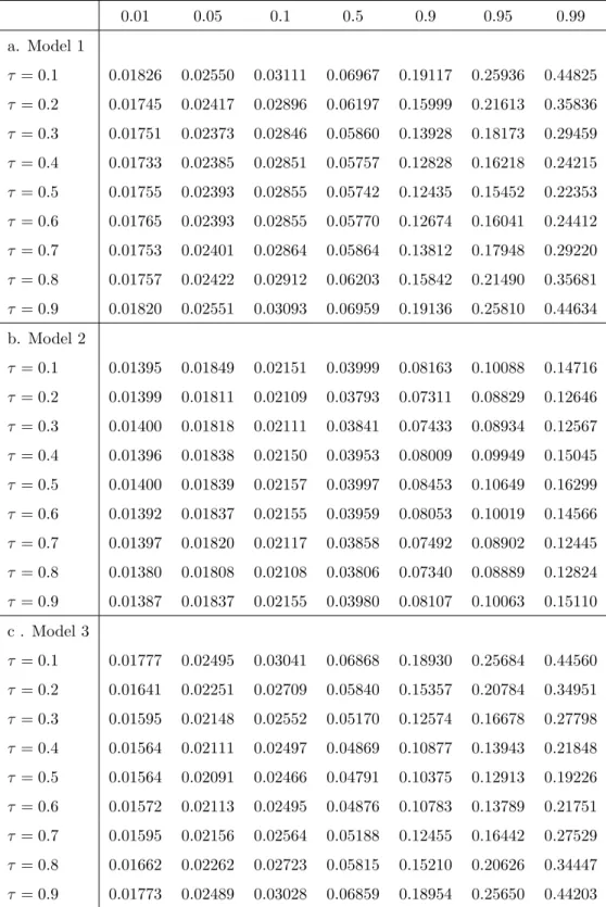
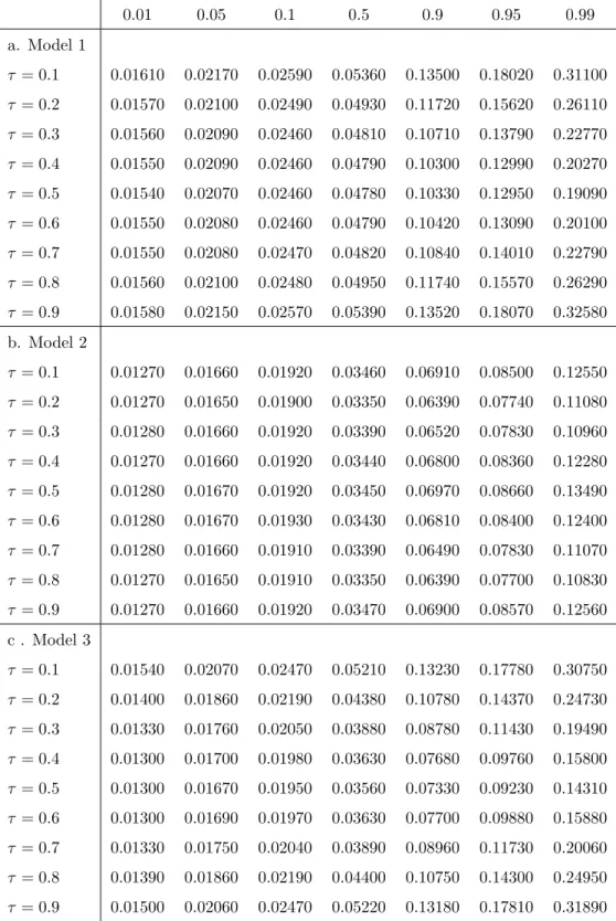
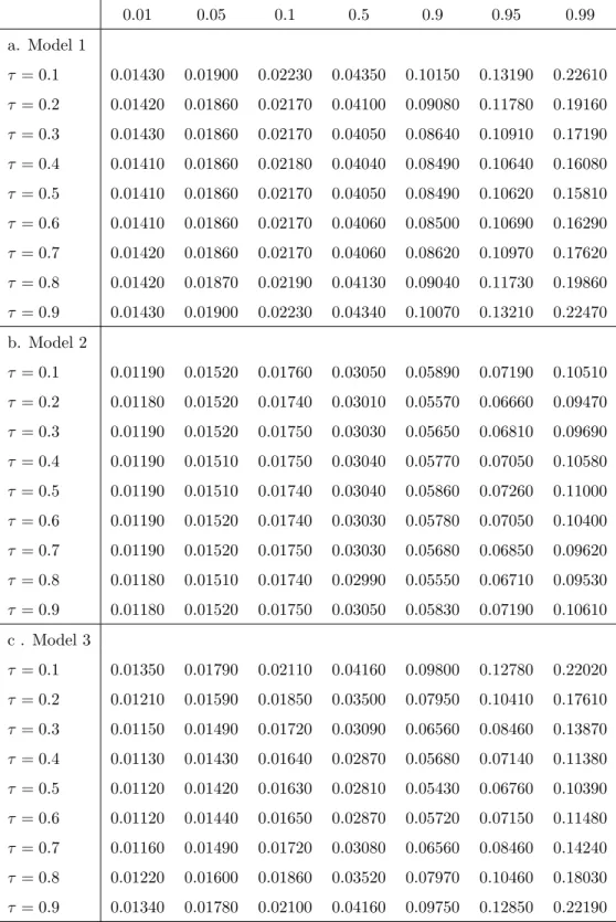
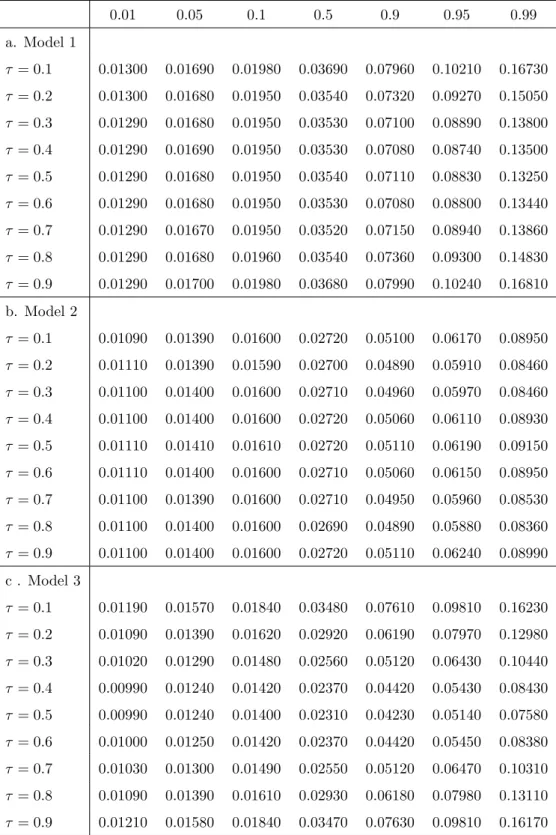
THEOREM 3.2 Suppose the conditions in Lemma 3.2 are satisfied. Then (i) under the null hy-pothesis Vnτ˜ has the same limiting distribution as Vnτ uniformly over τ ∈ [0,1]. (ii) Under the alternative,Vnτ˜ =Op(n/`).

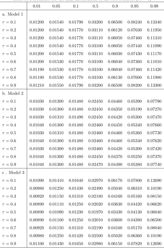
The first part of Theorem 3.2 implies that the test statistics based on models 1’–3’ have the same limiting distributions as those in Theorem 3.1 even if the I(1) regressors are not strictly exogenous. Critical values of the tests are calculated form= 1–5 in Tables 1–5, respectively. They are based on the representation of the limiting distributions in Theorem 3.1 wheremis the number of I(1) regressors. Each table is calculated for values ofτ = 0.1–0.9. The critical values are obtained from 50,000 replications at sample sizen= 2,000. The second part of Theorem 3.2 shows that the test is consistent. Indeed, the test statistic diverges to infinity at a rate (n/l) under the alternative. This result is analogous to that in Kwiatkowski et al. (1992) and Shin (1994), where the rate of divergence of the test statistics depends on the bandwidth parameter`. The consistency of the test proposed in Theorem 3.1 is straightforward, a special case of the second part of Theorem 3.2.

(12)

4 Testing the null of cointegration with structural breaks of

unknown timing

In this section, we generalize the results given in the last section to the case where a structural break occurs at unknown timing. When the location of the break point (or, equivalently, break fraction

τ) is unknown, we can employ two strategies. One is to first estimate the break fraction and then construct the test statistic by replacing the known fraction with the estimated one. The other is to construct the test statistic for all possible break points and then take the infimum of those statistics. In the framework of testing for stationarity with a structural break, the first method is suggested by Kurozumi (2002) while the second is proposed by Busetti & Harvey (2001).

To present the first test statistic and derive its asymptotic distribution, we need to begin by estimating the break fraction. Two types of estimators for the break fraction are present in the literature. One is the pseudo-Gaussian maximum likelihood estimator (MLE) proposed by Bai et al. (1998) and the other is the least squares estimator developed by Kurozumi & Arai (2005). Whereas Bai et al. (1998) show detailed limiting properties (including the limiting distribution) of the pseudo-Gaussian MLE under restrictive assumptions, Kurozumi & Arai (2005) only show particular limting properties of the least squares estimator under much less restrictive assumptions. In this paper we employ the second estimator because some of the assumptions made in Bai et al. (1998) are not very realistic. Moreover, as we shall see in the proof of Theorem 4.1, the properties given in Kurozumi & Arai (2005) are sufficient for our purpose. The estimator is defined by

ˆ

τ = arg inf

τ∈TSSRn(τ) (18)

where SSRn(τ) =Pn

t=1eˆ2tτ and ˆetτ is defined as before. The limiting properties of this estimator

are derived under the following assumption:3

ASSUMPTION 4.1 β2 in (12), (13) and (14) shrinks to zero as the sample size ngoes to infinity at the rate of n1/2_{, i.e.} _β

2=β2n =n−1/2β2o whereβ2o is a vector of constants.

Assumption 4.1 embodies the idea that the post-break coefficients of the integrated regressors shrink to the pre-break coefficients at a suitable rate. This is equivalent to considering that the magnitude of a shift is small and converges to zero as the sample size goes to infinity. Bai et al. (1998) convincingly explain three reasons for assuming this shift to be small. First, we can show some analytical properties of the estimated break point. This becomes important when we develop the limiting properties of the test statistics. Second, if we can consistently estimate the break point for a small shift, we should be able to estimate it consistently for a large shift. Third, if a shift in the

(13)

coefficients for the I(1) regressors does not converge to zero much faster than that for the intercept, the limiting behavior of the estimated break point will be dominated by the I(1) coefficients (see Bai et al., 1998 for more detailed explanations).

Now we are ready to propose a test statistic and show its limiting distribution. Let ˆτ be the estimated break fraction defined in (18) and estimate one of models 1–3 by OLS using modified regression model (12), (13) or (14). Denote the residual by ˜etτˆ. Note that this residual depends on the estimated change point ˆτ. Then the test statistic is given by

˜ Vnτˆ=n−2 n X t=1 ˜ S2_t_τ_ˆ/ω˜1·2ˆτ (19) where ˜Stˆτ = P t

s=1˜esτˆ and ˜ω1·2ˆτ is any consistent estimator of ω1·2 = ω11−ω021Ω22ω21. As an example, the standard semiparametric estimator based on ˜etτˆ would satisfy the requirement of con-sistency. The subscript ˆτ in ˜ω1·2ˆτ implies that the residual is from OLS estimation of the model

where the break fractionτ is estimated. The next theorem derives the limiting properties of the test statistic ˜Vnˆτ.

THEOREM 4.1 Suppose the conditions in Lemma 3.2 are satisfied. In addition, suppose Assump-tion 4.1 holds. Then, (i) under the null hypothesis as n→ ∞

˜

Vnτˆ−V˜nτ p

→0

uniformly overτ. (ii) Under the alternative, Vn˜ τˆ=Op(n/l).

The first part of Theorem 4.1 implies that the test statistic has the same limiting distribution given in Theorem 3.2, even if we use the estimated break fraction to construct it. Thus even if we do not know the timing of the structural break, by constructing the test statistic using the estimated break fraction, we can conduct a test for cointegration with structural breaks based on the same critical values as if the true break fraction was known. The second part of Theorem 4.1 shows that the test is consistent against the alternative.

Next we introduce the second type of test statistic. When the location of a break point is unknown in the context of testing for stationarity, Busetti and Harvey (2001) propose an approach to construct a test statistic such that the break point is chosen to be most favorable for the null hypothesis.4 _{We apply this approach to the test of cointegration with structural breaks. As in} Busetti & Harvey (2001), we assume the following instead of Assumption 4.1:

ASSUMPTION 4.2 We assume µ2 = µ2n = o(n−1/2) for models 1 and 2, and µ2 = µ2n = op(n−1/2₎_and_β

(14)

Assumption 4.2 implies that we need to impose stronger conditions on how µ2n and β2n shrink to

zero as the sample sizengoes to infinity. The test statistic is proposed by

Vn def = inf τ≤τ≤¯τ ˜ Vnτ = inf τ≤τ≤¯τ n −2 n X t=1 ˜ S_tτ2/ω˜1·2τ ! .

THEOREM 4.2 Let the conditions in Lemma 3.2 be satisfied. In addition, suppose Assumption 4.2 holds. Then, (i) under the null hypothesis,

inf τ≤τ≤τ¯ ˜ Vnτ ⇒ inf τ≤τ≤¯τ Z 1 0 Q2_τ(r)dr,

whereQτ(r) is given in Theorem 3.1. (ii) Under the alternative, the test statistic isOp(n/`).

5 Simulation Evidence

In this section we investigate finite sample properties of the test statistics. The data generating processes in our experiments are

y1t = 1 +µ2ϕtτ+ 2y2t+et (model 1), y1t = 1 +µ2ϕtτ+ 0.2t+ 2y2t+et (model 2), y1t = 1 +µ2ϕtτ+ 2y2t+β2y2tϕtτ+et (model 3)

where the dimension ofy2t(m) is equal to one,

et = γt+v1t,

y2t = y2,t−1+v2t, γt = γt−1+ut,

vt = Avt−1+t,

withA=diag{a11, a22},t∼i.i.d.N(0, I2) andut∼i.i.d.N(0, σu2) independent of{s}for alls. We

seta11=a22= 0,±0.4 or±0.8,σu2= 0, 0.01, 0.1, 1 or 10, and sample sizen= 100 or 200. The break

fraction τ is primarily set at 0.5 and other values are discussed briefly without providing results.5 The values of µ2 and β2 are discussed and specified later. We use the semiparametric consistent estimator defined by (17) with the Bartlett kernel k(s/`) = 1−s/(`+ 1). We use three kinds of bandwidth parameter`: `4= [4(n/100)1/4] and`12= [12(n/100)1/4] as used by Schwert (1989) and Kwiatkowski et al. (1992), while the third choice `a is a truncated version of the data-dependent

(15)

method proposed by Andrews (1991) and used by Arai (2004) and Kurozumi (2002):6 `a= min 1.1447 _{4 ˆ}_ρ2_n (1 + ˆρ)2₍₁₋_ρ_ˆ₎2 1/3 ,1.1447 ₄ ×0.92_n (1 + 0.9)2₍₁₋₀_.₉₎2 1/3! ,

where ˆρis the coefficient estimated by the first order autoregression ofε∗_t. The number of leads and lags used to estimate the parameters is determined by aF test for the significance of leads and lags with a maximum lag length `4.7 The level of significance is 0.05 and the number of replications is 1,000 in all experiments.

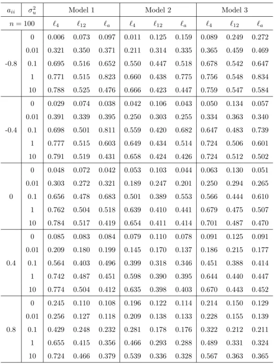
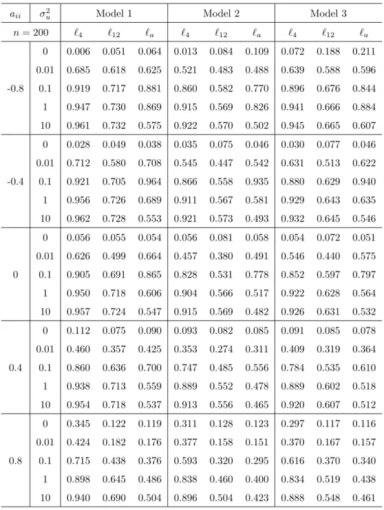
For the known break point case the test statistics are invariant to the true values of the coefficients soµ2andβ2can be set to zero without loss of generality. Results are tabulated in Tables 6 and 7. On the whole, the empirical size of the test is close to the nominal one unless|aii|is large,

in which case the test tends to be oversized, especially whenn= 100. The bandwidth of`4is enough for the test to have an empirical size close to 0.05 whenaii is small, but a bandwidth such as `12 or `a is required for the empirical size of the test to be close to the nominal one for large aii. The test tends to be more powerful for larger n and smaller |aii|. We also note that power does not necessarily increase asσ2

uincreases, especially whenσu2 is greater than 1 and`a is used. The reason

is that a unit root process γt dominates the other stationary components whenσ_u2 is large (even in small samples), and then the longer bandwidth in `a tends to be chosen. Hence the power of the test decreases as predicted by the second part of Theorem 3.2.

[Tables 6 and 7 around here]

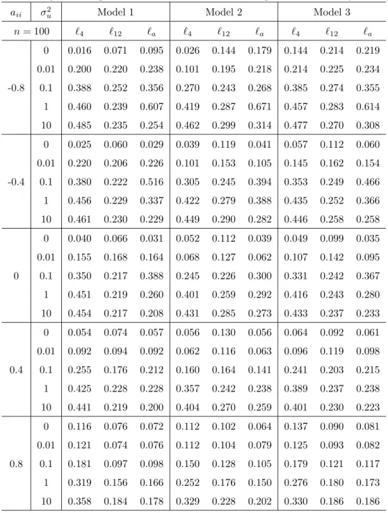
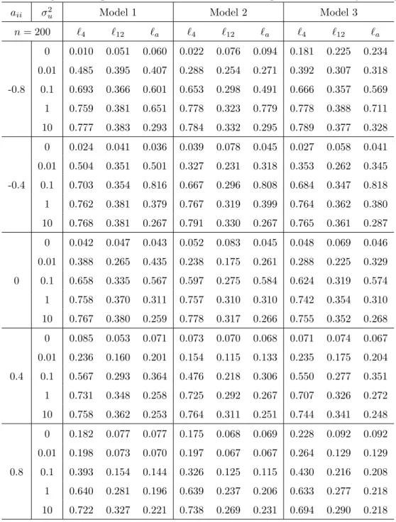
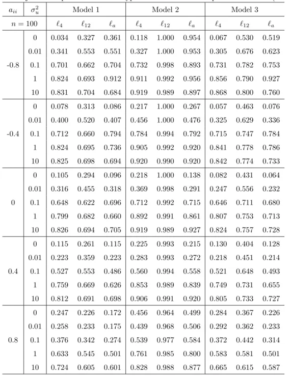
For the unknown break point case the finite-sample properties of the test statistics are affected by the magnitude of the break and so we consider two cases: for models 1 and 2 we set µ2 = 1.1 for a small shift and µ2 = 2.2 for a large shift for all sample sizes. For model 3 {µ2, β2} are set equal to {0.4,0.1} and {0.8,0.2} for a small and large shift when n = 100, while they are

{0.2,0.09} and {0.4,0.18} when n = 200. These parameters are chosen so that the magnitude of the change is about equal to a half or one standard deviation of y1,t+1, for a respective small or large shift. Note that the component of variation iny1,t+1 giveny1t is 2v2,t+1+et+1, with variance Var(2v2,t+1+et+1) = 4 + 1 = 5 when {vt}is an i.i.d. sequence, such that a half standard deviation is 0.5×√5'1.1. Then, for example, since the magnitude of the break is µ1 for models 1 and 2, it is set equal to 1.1 for the small shift case. For model 3, the magnitude of the break is µ2+β2y2,51 when n = 100 and since the standard deviation of β2y2,51 is

√

51β2, we set µ2 and β2 such that

µ2+

√

51β2'1.1 for the small magnitude case. [Tables 8 and 9 around here]

(16)

report only the small shift case because the results for the large shift case turns out to be very similar in our unreported simulation results. The size of the test is close to the nominal one when`a is used (except for the case whereaii=−0.8), but the power of the test is low whenaiiis large andn= 100. On the whole, the bandwidth parameter`4 is not a suitable choice for largeaii. We also conducted simulations forT =T2 = [0.15,0.85]. Unreported results show that the small sample properties of the proposed tests are not significantly affected by the choice ofT.

[Tables 10 and 11 about here]

The results for the inf-type test are summarized in Tables 10 and 11.8 _{The empirical sizes are} rarely below 0.10. Since the size distortions are very large even forn= 200, we do not recommend using these statistics when structural changes are considered in the model.

We now study the effect produced by the location of the break point. We conduct the same experiments as above for different values of τ: 0.05, 0.25, 0.75 and 0.95. The results are roughly symmetric aroundτ= 0.5. There is no strong tendency for the finite-sample properties of a specific value ofτ to be any better than those for other values. For example, the differences in the empirical sizes are never larger than 0.04 unless we use`12 in model 3 with known timing. These properties are preserved in the case when the break point is unknown. Hence we conclude that the effect of the location of the break point is small.

6 Concluding Remarks

In this paper we have developed residual-based tests for the null hypothesis of cointegration with structural breaks against the alternative hypothesis of no cointegration. The LM test statistic is derived and its limiting distribution is obtained for the case where the timing of a structural break is known. Then it is generalized to accommodate a structural break of unknown timing in two ways. The limiting properties of both statistics are studied under the null as well as the alternative. Finite-sample simulations show that the empirical size of the test is close to the nominal one unless the regression error is very persistent. Additionally, the test rejects the null when no cointegrating relationship with a structural break is present. It is also revealed in our limited set of simulations that the “Inf-type” statistic proposed for the case where a structural break occurs at unknown timing suffers large size distortions and hence is not very useful in practice.

(17)

APPENDIX A

Throughout the proof, ⇒ denotes weak convergence of the associated probability measure with respect to the uniform metric overτ ∈[0,1] orτ ∈ T whereT = [τ ,τ¯], 0< τ <¯τ <1. Remember that ξt = P

t

s=1vs is the partial sum of the innovations vt and B(r) is an (m+ 1)-dimensional

Brownian motion. Partitionξt= (ξ1t, ξ20t)0 andB(r) = (B1(r), B2(r)0)0 in conformity withvt. The

following lemma, which we state without proof, is fundamental for our proof.

LEMMA 6.1 (Gregory & Hansen, 1996) Under Assumption 3.1, the following joint weak con-vergence holds (a) 1 n3/2 n X t=[nτ] ξt⇒ Z 1 τ B(r)dr, (b) 1 n2 n X t=[nτ] ξtξt⇒ Z 1 τ B(r)B(r)0dr, (c) 1 n n X t=[nτ] ξtv0t+1⇒ Z 1 τ B(r)dB(r)0+ (1−τ)Λ.

Following Gregory & Hansen (1996), we refer to results such as (a), (b) and (c) in Lemma 6.1 as holding “uniformly overτ”.

Proof of Lemma 3.1: We provide a rigorous proof for model 3. A proof for model 1 is a special case of that for model 3 and that for model 2 is a simple extension of that for model 3. For model 3, we haveb = (µ1, µ2, β01, β20)0 and Dn = n1/2, n1/2, nIm, nIm

as defined in Section 3. Then the OLS estimator ofbis given by

ˆ_bτ ₌ n X t=1 XtτXtτ0 !−1 n X t=1 Xtτy1t ! whereXtτ = (1, ϕtτ, y20t, y20tϕtτ) 0

. This implies that under the null hypothesis

Dnˆbτ−b=Dn n X t=1 XtτXtτ0 !−1 DnD−n1 n X t=1 Xtτv1t ! or equivalently Dn ˆ bτ−b =

(18)

        1 n−1Pn t=1ϕtτ n− 3/2Pn t=1y02t n− 3/2Pn t=1y02tϕtτ n−1Pn t=1ϕtτ n− 1Pn t=1ϕtτ n− 3/2Pn t=1y02tϕtτ n− 3/2Pn t=1y02tϕtτ n−3/2Pn t=1y2t n−3/2P n t=1y2tϕtτ n−2P n t=1y2ty02t n−2 Pn t=1y2ty02tϕtτ n−3/2Pn t=1y2tϕtτ n−3/2P n t=1y2tϕtτ n−2P n t=1y2ty20tϕtτ n−2P n t=1y2ty02tϕtτ         −1 ×         n−1/2Pn t=1v1t n−1/2Pn t=1ϕtτv1t n−1Pn t=1y2tv1t n−1Pn t=1y2tϕtτv1t        

where we used the facts thatet=v1tunder the null andϕ2tτ =ϕtτ. It follows from Lemma 6.1 that

Dnˆbτ−bτ⇒         1 R1 0 ϕτ(r)dr R1 0 B2(r) 0_dr R1 0 B2(r) 0_ϕ τ(r)dr R1 0 ϕτ(r)dr R1 0 ϕτ(r)dr R1 0 B2(r) 0_ϕτ₍_r₎_dr R1 0 B2(r) 0_ϕτ₍_r₎_dr R1 0 B2(r)dr R1 0 B2(r)ϕτ(r)dr R1 0 B2(r)B2(r) 0_dr R1 0 B2(r)B2(r) 0_ϕτ₍_r₎_dr R1 0 B2(r)ϕτ(r)dr R1 0 B2(r)ϕτ(r)dr R1 0 B2(r)B2(r) 0_ϕτ₍_r₎_dr R1 0 B2(r)B2(r) 0_ϕτ₍_r₎_dr         −1 ×         B1(1) R1 0 ϕτ(r)dB1(r) R1 0 B2(r)dB1(r) R1 0 B2(r)ϕτ(r)dB1(r)         = Z 1 0 Xτ(r)Xτ(r)0dr −1Z 1 0 Xτ(r)dB1(r)

whereXτ(r) = (1, ϕτ(r), B2(r)0, B2(r)0ϕτ(r))0 for model 3, giving the required results. 2

Proof of Theorem 3.1: Using the notation given in the proof of Lemma 3.1, ˆStτ can be expressed as ˆ Stτ = t X s=1 ˆ esτ = t X s=1 y1s−ˆb0τXsτ = t X s=1 v1s− ˆ_bτ₋_b0 t X s=1 Xsτ

by noting thatet=v1tunder the null. It follows from Lemma 6.1 and Lemma 3.1 that

n−1/2Sˆ[nr]τ = n−1/2 [nr] X t=1 v1t− ˆ_b τ−b 0 DnD−n1n− 1/2 [nr] X t=1 Xtτ ⇒ B1(r)− Z r 0 Xτ(s)ds 0Z 1 0 Xτ(s)Xτ(s)0ds −1Z 1 0 Xτ(s)dB1(s) def = QXτ(r).

(19)

Define ΩX = diag (1,1,Ω22,Ω22) and remember that Qτ(r) =W1(r)− Z r 0 Wτ(s)ds 0Z 1 0 Wτ(s)Wτ(s)0ds −1Z 1 0 Wτ(s)dW1(s) .

where Wτ(r) = (1, ϕτ(r), W2(r)0, W2(r)0ϕτ(r))0 and W2(r) is anm-dimensional standard Brownian motion independent of a scalar-valued Brownian motionW1(r). Then we get

QXτ(r)=d ω1₁₁/2W1(r) −ω1₁₁/2 Z r 0 Wτ(s)ds 0 Ω1_X/2Ω−_X1/2 Z 1 0 Wτ(s)Wτ(s)0ds −1 Ω−_X1/2Ω1_X/2 Z 1 0 Wτ(s)dW1(s) = ω₁₁1/2Qτ(r)

where “=” signifies equality in distribution. Since ˆd ω11τ is a consistent estimator ofω11, we have

Vnτ =n−2 n X t=1 ˆ S_tτ2/ωˆ11τ ⇒ Z 1 0 Q2_τ(r)dr.

If we use the semiparametric estimator given in (11), its consistency can be shown as in Shin (1994) under general regularity conditions. 2

Proof of Lemma 3.2: Note that we now haven−2K observations, but we will useninstead of

n−2Kwithout loss of generality. Denote

π = (π0₋_K, π0₋_K₊₁, . . . , π0_K₋₁, π_K0 )0, γ = (b0, π0)0, ZtK = (∆y₂0_,t₋_K,∆y₂0_,t₋_K₊₁, . . . ,∆y₂0_,t₊_K₋₁,∆y0₂_,t₊_K)0, Utτ = (X_tτ0 , Z_tK0 )0 D∗_n = diag(n1/2Im, . . . , n1/2Im) and Dn˜ = diag(Dn, D_n∗)

whereXtτ is defined as in Lemma 3.1 and dependence ofUtτ onKis suppressed for simplicity. Also let the OLS estimator ofπandγ be ˜πτ and ˜γτ respectively. We have

˜ Dn(˜γτ−γ) = Dn˜ n X t=1 UtτU_tτ0 !−1 ˜ DnD˜−_n1 n X t=1 Utτε∗_t ! = R˜−1D˜_n−1 n X t=1 Utτε∗_t ! (20) where ˜ R=   D−1 n Pn t=1XtτXtτ0 Dn−1 Dn−1 Pn t=1XtτZtK0 D ∗ n −1 D∗_n−1Pn t=1ZtKXtτ0 Dn−1 D∗n −1Pn t=1ZtKZtK0 D∗n −1  .

(20)

Define R=   D−1 n Pn t=1XtτXtτ0 Dn−1 0 0 E(ZtKZ_tK0 )  .

Lemma A4 of Saikkonen (1991) shows that

˜ R−1−R−1 ₁=Op K/T1/2

where || · ||1 is the matrix norm ||A||1 = sup{||Ax||:||x|| ≤1} and|| · || is the standard Euclidean norm. DefineηtK=Pj>|K|πjv2,t−j. SinceRis block diagonal, (20) implies

Dn˜bτ−b = Dn n X t=1 XtτX_tτ0 !−1 DnD_n−1 n X t=1 Xtτε∗_t ! +op(1) = Dn n X t=1 XtτXtτ0 !−1 DnDn−1 n X t=1 Xtτεt ! +Dn n X t=1 XtτXtτ0 !−1 DnD−n1 n X t=1 XtτηtK ! +op(1). (21)

It was shown in the proof of Lemma 3.1 that

Dn n X t=1 XtτXtτ0 !−1 Dn=Op(1). (22)

Definewt= (εt, v₂0_t)0. Note that we have assumed that (εt, v₂0_t)0 satisfies Assumption 3.1. Then the multivariate invariance principle holds:

n−1/2

[nr]

X

t=1

wt⇒B˜(r)

where ˜B(r) = (B1·2(r), B2(r)0)0 is an (m+ 1)-dimensional Brownian motion with covariance matrix ˜

Ω = diag(ω1·2,Ω22),ω1·2=ω11−ω210 Ω22ω21, andB1·2(r) andB2(r) denote Brownian motions of 1 andmdimensions respectively. By Lemma 6.1, we have

D−n1 n X t=1 Xtτεt⇒ Z 1 0 Xτ(r)dB1·2(r) (23)

uniformly overτ. (A12) in Saikkonen (1991) also shows that

D_n−1 n X t=1 XtτηtK =op(1). (24)

Combining (21), (22), (23) and (24) gives the result required for the first part of Lemma 3.2. The second part of Lemma 3.2 is shown by Saikkonen (1991, pp.21). 2

(21)

Proof of Theorem 3.2: Using the notation given in the proof of Lemma 3.2, ˜Stτ can be expressed as ˜ S[nr]τ = [nr] X t=1 ˜ etτ = [nr] X t=1 y1t−˜b0τXtτ−π˜ 0 τZtK = [nr] X t=1 εt+ [nr] X t=1 ηtK− ˜_b τ−bτ 0 [nr] X t=1 Xtτ−(˜πτ−π) 0 [nr] X t=1 ZtK.

It follows from Lemma 6.1, and Lemma 3.2 that

n−1/2S˜[nr]τ = n−1/2 [nr] X t=1 εt+n−1/2 [nr] X t=1 ηtK −ˆbτ−b 0 DnD_n−1n−1/2 [nr] X t=1 Xtτ−(˜πτ−π)0n−1/2 [nr] X t=1 ZtK ⇒ B1·2(r)− Z r 0 Xτ(s)ds 0Z 1 0 Xτ(s)Xτ(s)0ds −1Z 1 0 Xτ(s)dB1·2(s) def = Q˜Xτ(r), if we have sup 0≤r≤1 n−1/2 [nr] X t=1 ηtK = op(1), sup 0≤r≤1 (˜πτ−π)0n−1/2 [nr] X t=1 Zt = op(1). (25)

These were shown in the proof of Theorem 2 by Shin (1994, p.113). Define ΩX= diag (1,1,Ω22,Ω22) and remember that

Qτ(r) =W1(r)− Z r 0 Wτ(s)ds 0Z 1 0 Wτ(s)Wτ(s)0ds −1Z 1 0 Wτ(s)dW1(s) . Then we get ˜ QXτ(r)=d ω1₁/_·₂2W1(r) −ω1₁/_·₂2 Z r 0 Wτ(s)ds 0 Ω1_X/2Ω−_X1/2 Z 1 0 Wτ(s)Wτ(s)0ds −1 Ω−_X1/2Ω1_X/2 Z 1 0 Wτ(s)dW1(s) = ω₁1_·/₂2Qτ(r).

Since ˆω1·2 is a consistent estimator ofω1·2, we have

˜ Vnτ =n−2 n X t=1 ˜ S_tτ2/ω˜1·2⇒ Z 1 0 Q2_τ(r)dr,

(22)

proving the first part of Theorem 3.1.

To show the second part, we derive the convergence rate of (˜bτ−b) and (˜πj−πj) under the alternative. As in the proof of Lemma 3.2, we have

˜ Dn(˜γτ−γ) = ˜R−1D˜_n−1 n X t=1 Utτ(γt+ε∗_t)

under the alternative. Since ˜R is the same as under the null hypothesis, we can investigate ˜bτ

separately from ˜πτ as we did in the proof of Lemma 3.2. Noting that

D−_n1 n X t=1 Xtτ(γt+ε∗_t) =D_n−1 n X t=1 Xtτ(γt+εt+ηtK),

we can see thatD_n−1Pn

t=1Xtτγtis of ordernand dominates the other terms. Then we have

Dn(˜bτ−b) =Op(n), (26)

under the alternative.

To derive the convergence rate of (˜πj −πj) under the alternative, let us define ˜R22 =

D∗−1

n

Pn

t=1ZtKZtK0 D

∗−1

n andR22=E(ZtKZtK0 ). Since ˜Ris asymptotically block diagonal,||D

∗ n(˜πτ− π)||is asymptotically equivalent to||R˜−₂₂1D∗−1 n Pn t=1ZtK(γt+ε∗t)||. Note that ||R˜−₂₂1D∗−_n 1 n X t=1 ZtK(γt+ε∗_t)|| ≤ ||R˜−₂₂1−R₂₂−1||1||Dn∗−1 n X t=1 ZtK(γt+ε∗t)||+||R− 1 22||1||Dn∗−1 n X t=1 ZtK(γt+ε∗t)||. Since n−1/2 n X t=1 v2,t−j(γt+ε∗t) =Op(n 1/2₎_, we have ||D_n∗−1 n X t=1 ZtK(γt+ε∗_t)||=Op(K1/2n1/2).

Using this result and the following results shown by Saikkonen (1991)

||R˜₂₂−1−R−₂₂1||1=Op(K/n1/2) and ||R−221||1=Op(1),

we can show that

||D∗_n(˜πτ−π)||=Op(K1/2n1/2).

Then it follows by noting||D∗n(˜πτ−π)||=n1/2(

PK j=−K||πj˜ −πj|| 2₎1/2_that K X j=−K ||πj˜ −πj||2₌_Op₍_K₎_. ₍₂₇₎

(23)

Next, we consider the partial sum of the regression residuals ˜etτ, [nr] X t=1 ˜ etτ = [nr] X t=1 (y1t−˜b0τXtτ−π˜τ0ZtK) = [nr] X t=1 n γt+εt+ηtK−(˜bτ−b)0DnDn−1Xtτ −( ˜πτ−π)0ZtK o . (28)

Observe that we have by (27)

sup 0≤r≤1 |(˜πτ−π)0Z[nr]K| ≤ sup 0≤r≤1 n (˜πτ−π)0(˜πτ−π)(Z[0nr]KZ[nr]K) o1/2 = sup 0≤r≤1   K X j=−K ||π˜j−πj||2 K X j=−K ||v2,[nr]−j||2   1/2 ≤ (2K+ 1)1/2 sup 0≤r≤1 ||v2[nr]||   K X j=−K ||πj˜ −πj||2   1/2 = Op(K). (29)

Then it follows by (26) and (29) that the first and fourth terms in (28) dominate the other terms and are of ordern3/2_{, such that}P[nr]

t=1e˜tτ =Op(n3/2). Then we have n X t=1   t X j=1 ˜ ejτ   2 =Op(n4).

In the same way as Kwiatkowski et al. (1992) and Phillips (1991), we can also see that

n−1Pn−j

t=1 ˜etτ˜et+j,τ =Op(n) and then ˜ω1·2τ =Op(`n) under some general regularity conditions on

k(·). Then the order of ˜Vnτ becomes n−2_×_Op₍_n4₎_×_Op₍_`−1_n−1_{) =}_Op₍_n/`_). ₂

Proof of Theorem 4.1: We note that b is now defined as b = (µ1, µ2n, β10, β20n)0. Let ˜bτ and ˜πτ

be defined as in the proof of Lemma 3.2 and also let ˜bˆτ and ˜πˆτ be the OLS estimates of b and π

obtained using the estimated change point ˆτ. First we show the following lemma.

LEMMA 6.2 Let Assumption 3.1 and 4.1 hold. Then we have, as n→ ∞

(i)n−1/2P[nr] t=1(ϕtτˆ−ϕtτ) p →0, (ii) n−1P[nr] t=1y2t(ϕtτˆ−ϕtτ) p →0, (iii)n−3/2P[nr] t=1y2ty02t(ϕtτˆ−ϕtτ) p →0, (iv)n−1/2P[nr] t=1v1t(ϕtτˆ−ϕtτ) p →0, (v)n−1P[nr] t=1y2tv1t(ϕtτˆ−ϕtτ) p →0, (vi)Dn˜bτˆ−˜bτ _p →0.

(24)

Proof of Lemma 6.2: (i) Without loss of generality we shall assume thatnτ andnτˆare integers. We have n−1/2 [nr] X t=1 (ϕtτˆ−ϕtτ) ≤ n 1/2_(ˆ_τ₋_τ₎ p →0

by Proposition 3 of Kurozumi & Arai (2005). (ii) We get n−1 [nr] X t=1 y2t(ϕtτˆ−ϕtτ) ≤ sup 0≤r≤1 y2[nr] n1/2 n 1/2_(ˆ_τ −τ) p →0 because sup₀_≤_r_≤₁y2[nr]/n1/2 =Op(1).

(iii)-(v) can be proved in the same way as (ii). To prove (vi), observe that

Dn˜bτˆ−˜bτ =Dn    n X t=1 XtτXˆ t0τˆ !−1 _n X t=1 Xtτyˆ 1t− n X t=1 XtτX_tτ0 !−1 _n X t=1 Xtτy1t    +op(1) (30)

by the argument used to prove Lemma 3.2. The required result follows if we show

Dn−1 n X t=1 XtτXˆ t0τˆ− n X t=1 XtτXtτ0 ! D−n1 p →0 (31) and D−_n1 n X t=1 (Xtτˆ−Xtτ)v1t p →0. (32) Noting that XtτˆXt0ˆτ−XtτX 0 tτ = (Xtˆτ−Xtτ)Xt0τˆ+Xtτ(Xtτˆ−Xtτ)0 and (Xtτˆ−Xtτ)0= [0,(ϕtˆτ−ϕtτ),0, y02t(ϕtτˆ−ϕtτ)]0,

we can show (31) using Lemma 6.2 (i), (ii) and (iii). Similarly, (32) follows by Lemma 6.2 (iv) and (v).

To prove the main result, it is sufficient to show that

sup 0≤r≤1 n −1/2_S_˜ [nr]ˆτ−n−1/2S[nr]τ p →0 (33) and ω˜1·2ˆτ−ω1·2τ p →0. (34)

Using the notation given above, ˜S[nr]τ and ˜S[nr]ˆτ can be written as

˜ S[nr]τ= [nr] X s=1 ˜ esτ = [nr] X s=1 y1s−˜b0τXsτ −π˜τ0ZsK

(25)

and ˜ S[nr]ˆτ = [nr] X s=1 ˜ esτˆ= [nr] X s=1 y1s−˜b0τˆXsˆτ−π˜0τˆZsK .

Then it follows that

n−1/2S˜[nr]ˆτ−n−1/2S˜[nr]τ = − ˜_b_τ_ˆ₋_b0_Dn    n−1/2D−_n1 [nr] X s=1 (Xsτˆ−Xsτ)    −b0n−1/2 [nr] X s=1 (Xsτˆ−Xsτ) −˜bτˆ−˜bτ 0 Dn    n−1/2D−_n1 [nr] X s=1 Xsτ    −(˜πτˆ−π˜τ) 0 n−1/2 [nr] X s=1 ZsK. (35)

To show (33), it suffices to show that each term in (35) converges to zero in probability uniformly over r∈ [0,1]. It follows by (i), (ii) and (vi) of Lemma 6.2 that the first term in (35) vanishes in probability as n → ∞. For the second term in (35), we have by Assumption 4.1, (i) and (ii) of Lemma 6.2 that b0n−1/2 [nr] X s=1 (Xsτˆ−Xsτ) =µ2nn−1/2 [nr] X s=1 (ϕsˆτ−ϕsτ) +β20nn−1/2 [nr] X s=1 y2t(ϕsτˆ−ϕsτ) p →0.

The third term of (35) converges to zero in probability by (a) of Lemma 6.1 and (vi) of Lemma 6.2. To show the convergence of the fourth term in (35), observe that the CLT and an argument similar to the one used to show Lemma 6.2 (vi) give

||D∗_n(˜πτˆ−˜πτ)||=op K1/2/n1/2 and n−1/2 [nr] X s=1 ZsK =OpK1/2.

Thus the fourth term also converges to zero in probability. Observing that all convergences shown above are uniform in r shows (33). (34) can be shown by noting that n1/2_(ˆ_τ ₋_τ_{) =} _o

p(1) by

Proposition 3 of Kurozumi & Arai (2005) and using standard arguments (see Shin (1994)). This finishes the proof of the first part of Theorem 4.1.

Proof of (ii): Let τ be an arbitrary break fraction and τo be the true one. Then the model can be expressed as

y1t=b0Xtτ +π0ZtK+γt+ε∗t −b

0₍_Xtτ ₋_Xtτ o),

(26)

whereb0(Xtτ−Xtτ_o) =µ2n(ϕtτ−ϕtτo) +β 0

2ny2t(ϕtτ−ϕtτo). We have by Assumption 4.1 and Lemma

6.1 that n X t=1 b0(Xtτ−Xtτ_o) =Op(n) (36) and n X t=1 y2tb0(Xtτ−Xtτo) =Op(n 3/2₎_. ₍₃₇₎

It can be deduced from (36) and (37) that

D−_n1 n X t=1 Xtτ{γt+ε∗_t−b0(Xtτ−Xtτ_o)} = D−_n1 n X t=1 Xtτγt+op(n) = Op(n).

As in the proof of Lemma 3.2, we can show that ˜Rbecomes asymptotically block diagonal and that (27) holds. Then we have by (27), (36) and (37) that

[nr] X t=1 ˜ etτ = [nr] X t=1 (y1t−˜b0τXtτ−π˜0τZtK) = [nr] X t=1 n γt+ε∗t−(˜bτ−b)0Xtτ −(˜πτ−π)0ZtK−b0(Xtτ−Xtτo) o = [nr] X t=1 γt−(˜bτ−b)0DnD−n1 [nr] X t=1 Xtτ +op(n3/2) = Op(n3/2)

under the alternative. This implies that Pn

t=1(

Pt

j=1e˜jτ)2 is of order n4. We can also show that

˜

ω1·2τ=Op(`n) as in the known break point case. Therefore ˜Vnτ =Op(n/`). Since this relation holds

for anyτ, the theorem is proved. 2

Proof of Theorem 4.2: In this proof, letτoandτ be the true break fraction and the fraction that

is used for estimation, respectively. We first show that (˜bτ−b) has the same asymptotic properties

as (˜bτo−b) in Lemma 3.2. Since the model is expressed as

y1t=b0Xtτ+π0ZtK+ε∗t−b

0₍_Xtτ₋_Xtτ o),

we can proceed the same way we did in Lemma 3.2, withε∗_t replaced byε∗_t −b0(Xtτ −Xtτ_o). Since

b0(Xtτ−Xtτ_o) =µ2n(ϕtτ −ϕtτo) +β 0

(27)

we can see that D_n−1 n X t=1 Xtτ(Xtτ−Xtτ_o)0b =         n−1/2Pn t=1{µ2n(ϕtτ−ϕtτo) +β 0 2ny2t(ϕtτ −ϕtτo)} n−1/2Pn t=1ϕtτ{µ2n(ϕtτ−ϕtτo) +β 0 2ny2t(ϕtτ −ϕtτo)} n−1Pn t=1y2t{µ2n(ϕtτ−ϕtτo) +β 0 2ny2t(ϕtτ−ϕtτo)} n−1Pn t=1y2tϕtτ{µ2n(ϕtτ−ϕtτo) +β 0 2ny2t(ϕtτ−ϕtτo)}         p → 0,

where the convergence is established because

n−1/2 n X t=1 {µ2n(ϕtτ −ϕtτo) +β 0 2ny2t(ϕtτ−ϕtτo)} ≤ n−1/2 n X t=1 |µ2n(ϕtτ−ϕtτo)|+n −1/2 n X t=1 |β₂0_ny2t(ϕtτ −ϕtτo)| ≤ n1/2|µ2n|+ sup 0≤r≤1 y2[nr] n1/2 n|β2n| p →0

by Assumption 4.2. This implies thatDn(˜bτ−b) has the same limiting distribution as that in Lemma 3.2. Similarly, we can show thatPK

j=−K||πj˜ −πj||2=Op(K/n) in the same way we did in Lemma

3.2.

Next, note that

˜ etτ = y1t−˜b0τXtτ−π˜ 0 τZtK = εt+ηtK−(˜bτ−b)0Xtτ−(˜πτ−π)0ZtK−b0_τ o(Xtτ−Xtτo)

and that (˜bτ−b) has the same asymptotic properties as (˜bτo−b) in Lemma 3.2. Then, just as in

the proof of Theorem 3.2, we can show that ˜S[nr]τ converges weakly to ˜QXτ(r) and ˜ω1·2τ converges

to ω1·2 in probability, implying that ˜Vnτ ⇒R 1 0 Q

2

τ(r)dr. Then the theorem is established using the

continuous mapping theorem.

Consistency of the test statistic can be proved in the same way as in Theorem 3.2. 2

Notes

1_{Tests for cointegration with structural breaks of “known” timing are proposed by Saikkonen & L¨}_{utkepohl (2000),}

Hansen (2003) and L¨utkepohl et al. (2003).

2_{Although ˜}_π

(28)

3_{To prove Theorem 4.1 by using the pseudo-Gaussian MLE, we need to assume the following:} _ASSUMPTION

4.1’(a) The I(1) regressory2tsatisfies:

E _ty2 2i,t y2 2i,1+y22i,2+· · ·+y22i,t

≤M for allt≥1andi= 1, . . . , m.

(b)εt is independent of the regressors for all leads and lags. (c)πi= 0for alli >|K|whereKis a finite constant.

(d)µ2 and β2 in (12), (13) and (14) depend on the sample sizen. We denote them byµ2nand β2n. We assume

µ2n=δnµ0 for the models 1 and 2, and for the model 3,µ2n=µoδn,β2n=n−1/2βoδnwhereδn is a scalar such

thatδn=o(n−ρ)for0< ρ <1/4,µ0 is a constant scalar andβ0 is a constantm-vector. These assumptions are

obviously more restrictive than Assumption 4.1. Assumption 4.1’ (b) would not be very realistic among others as we note in the last section.

4_{We also consider the analogous approach to constructing a test statistic so as to give the least favorable result for}

the null as in Zivot & Andrews (1992). The test statistic is defined as sup_τ≤τ≤¯τV˜nτ where ˜Vnτ is as in (19) and we can show results similar to those in Theorem 4.2. However, we do not present them in this and subsequent sections because unreported simulation experiments show that the finite-sample performance of such a “sup-type” test statistic is dominated by the “inf-type” one.

5_{All unreported results are available upon request.} 6_{There are typos in the expression of}_`

AKin Kurozumi (2002, pp.81). The numerator of the second argument in parentheses must be multiplied by 4 as the above expression.

7_{We use a maximum lag length less than}_`

4whenτis close to the end points in order to obtain enough observations

for estimation.

8_{Asymptotic critical values are calculated by employing the method of MacKinnon (1991).}

References

Andrews, D. W. K. (1991) Heteroskedasticity and autocorrelation consistent covariance matrix esti-mation.Econometrica59, 817–858.

Arai, Y. (2004) Testing for linearity in regressions with I(1) processes. Discussion paper CIRJE-F-303, Faculty of Economics, University of Tokyo.

Bai, J., R. L. Lumsdaine, & J. H. Stock (1998) Testing for and dating common breaks in multivariate time series.Review of Economic Studies 65, 395–432.

Brillinger, D. R. (1981) Time Series: Data Analysis and TheoryNew York: Holt, Rinehart and Winston.

Busetti, F. & A. Harvey (2001) Testing for the presence of a random walk in series with structural breaks.Journal of Time Series Analysis 22, 127–150.

(29)

Engle, R. F. & C. W. J. Granger (1987) Co–integration and error correction: Representation, esti-mation and testing.Econometrica 55, 547–557.

Granger, C. W. J. (1983) Co–integrated and error–correcting models. Discussion Paper 83–13, De-partment of Economics, University of California, San Diego.

Granger, C. W. J. & T.-H. Lee (1989) Multicointegration.Advances in Econometrics 8, 71–84.

Gregory, A. W. & B. E. Hansen (1996) Residual–based tests for cointegration in models with regime shifts.Journal of Econometrics 70, 99–126.

Hansen, P. R. (2003) Structural changes in the cointegrated vector autoregressive model.Journal of Econometrics 114, 261–295.

Herrndorf, N. (1984) A functional central limit theorem for weakly dependent sequences of random variables.Annals of Probability 12, 141–153.

Inoue, A. (1999) Tests of cointegrating rank with a trend–break.Journal of Econometrics 90, 215– 237.

Johansen, S. (1988) Statistical analysis of cointegration vectors.Journal of Economic Dynamics and Control 12, 231–254.

Johansen, S. (1991) Estimation and hypothesis testing of cointegration vectors in Gaussian vector autoregressive models.Econometrica 59, 1551–1580.

Kurozumi, E. (2002) Testing for stationarity with a break.Journal of Econometrics 108, 63–99.

Kurozumi, E. & Y. Arai (2005) Efficient estimation and inference in cointegrating regressions with structural change. Discussion Paper No. 2004-9, Graduate School of Economics, Hitotsubashi University (http://www.econ.hit-u.ac.jp/˜kurozumi/paper/efficientjan05.pdf).

Kwiatkowski, D., P. C. B. Phillips, P. Schmidt, & Y. Shin (1992) Testing the null hypothesis of stationarity against the alternative of a unit root.Journal of Econometrics 54, 159–178.

L¨utkepohl, H., P. Saikkonen, & C. Trenkler (2003) Comparison of tests for the cointegrating rank of a VAR process with a structural shift.Journal of Econometrics 113, 201–229.

L¨utkepohl, H., P. Saikkonen, & C. Trenkler (2004) Testing for the cointegrating rank of a VAR processes with level shift at unknown time.Econometrica72, 647–662.

(30)

MacKinnon, J. G. (1991) Critical values for cointegration tests. In R. F. Engle & C. W. J. Granger (eds.),Long-Run Economic Relationships, New York, pp. 267–276. Oxford University Press.

Nabeya, S. & K. Tanaka (1988) Asymptotic theory of a test for the constancy of regression coefficients against the random walk alternative.Annals of Statistics 16, 218–235.

Newey, W. K. & K. D. West (1987) A simple, positive semidefinite, heteroskedasticity and autocor-related consistent covariance matrix.Econometrica 55, 586–591.

Phillips, P. C. B. (1991) Spectral regression for cointegrated time series. In W. Barnett (ed.), Non-parametric and SemiNon-parametric Methods in Economics and Statistics, pp. 413–435. New York: Cambridge University Press.

Phillips, P. C. B. & S. N. Durlauf (1986) Multiple time series regression with integrated processes. Review of Economic Studies 53, 473–496.

Phillips, P. C. B. & S. Ouliaris (1990) Asymptotic properties of residual based tests for cointegration. Econometrica 58, 165–193.

Quintos, C. E. (1997) Stability tests in error correction models.Journal of Econometrics82, 289–315.

Saikkonen, P. (1991) Asymptotically efficient estimation of cointegration regressions. Econometric Theory 7, 1–21.

Saikkonen, P. & H. L¨utkepohl (2000) Testing for the cointegrating rank of a VAR process with structural shifts.Journal of Business and Economic Statistics 18, 451–464.

Schwert, G. W. (1989) Tests for unit roots: A monte carlo investigation. Journal of Business and Economic Statistics 7, 147–159.

Seo, B. (1998) Tests for structural change in cointegrated systems regressions. Econometric The-ory 14, 222–259.

Shin, Y. (1994) A residual–based test of the null of cointegration against alternative of no cointegra-tion.Econometric Theory 10, 91–115.

Zivot, E. & D. W. K. Andrews (1992) Further evidence on the great crash, the oil-price shock, and the unit-root hypothesis.Journal of Business and Economic Statistics 10, 251–270.

(31)

Table 1: Percentiles for the null distribution of the test statistic (m= 1) 0.01 0.05 0.1 0.5 0.9 0.95 0.99 a. Model 1 τ = 0.1 0.01826 0.02550 0.03111 0.06967 0.19117 0.25936 0.44825 τ = 0.2 0.01745 0.02417 0.02896 0.06197 0.15999 0.21613 0.35836 τ = 0.3 0.01751 0.02373 0.02846 0.05860 0.13928 0.18173 0.29459 τ = 0.4 0.01733 0.02385 0.02851 0.05757 0.12828 0.16218 0.24215 τ = 0.5 0.01755 0.02393 0.02855 0.05742 0.12435 0.15452 0.22353 τ = 0.6 0.01765 0.02393 0.02855 0.05770 0.12674 0.16041 0.24412 τ = 0.7 0.01753 0.02401 0.02864 0.05864 0.13812 0.17948 0.29220 τ = 0.8 0.01757 0.02422 0.02912 0.06203 0.15842 0.21490 0.35681 τ = 0.9 0.01820 0.02551 0.03093 0.06959 0.19136 0.25810 0.44634 b. Model 2 τ = 0.1 0.01395 0.01849 0.02151 0.03999 0.08163 0.10088 0.14716 τ = 0.2 0.01399 0.01811 0.02109 0.03793 0.07311 0.08829 0.12646 τ = 0.3 0.01400 0.01818 0.02111 0.03841 0.07433 0.08934 0.12567 τ = 0.4 0.01396 0.01838 0.02150 0.03953 0.08009 0.09949 0.15045 τ = 0.5 0.01400 0.01839 0.02157 0.03997 0.08453 0.10649 0.16299 τ = 0.6 0.01392 0.01837 0.02155 0.03959 0.08053 0.10019 0.14566 τ = 0.7 0.01397 0.01820 0.02117 0.03858 0.07492 0.08902 0.12445 τ = 0.8 0.01380 0.01808 0.02108 0.03806 0.07340 0.08889 0.12824 τ = 0.9 0.01387 0.01837 0.02155 0.03980 0.08107 0.10063 0.15110 c . Model 3 τ = 0.1 0.01777 0.02495 0.03041 0.06868 0.18930 0.25684 0.44560 τ = 0.2 0.01641 0.02251 0.02709 0.05840 0.15357 0.20784 0.34951 τ = 0.3 0.01595 0.02148 0.02552 0.05170 0.12574 0.16678 0.27798 τ = 0.4 0.01564 0.02111 0.02497 0.04869 0.10877 0.13943 0.21848 τ = 0.5 0.01564 0.02091 0.02466 0.04791 0.10375 0.12913 0.19226 τ = 0.6 0.01572 0.02113 0.02495 0.04876 0.10783 0.13789 0.21751 τ = 0.7 0.01595 0.02156 0.02564 0.05188 0.12455 0.16442 0.27529 τ = 0.8 0.01662 0.02262 0.02723 0.05815 0.15210 0.20626 0.34447 τ = 0.9 0.01773 0.02489 0.03028 0.06859 0.18954 0.25650 0.44203

(32)

(33)

(34)

(35)

(36)

Table 6: Rejection frequencies of the tests when the break point is known (n= 100)

aii σ2u Model 1 Model 2 Model 3 n= 100 `4 `12 à `4 `12 à `4 `12 à 0 0.006 0.073 0.097 0.011 0.125 0.159 0.089 0.249 0.272 0.01 0.321 0.350 0.371 0.211 0.314 0.335 0.365 0.459 0.469 -0.8 0.1 0.695 0.516 0.652 0.550 0.447 0.518 0.678 0.542 0.647 1 0.771 0.515 0.823 0.660 0.438 0.775 0.756 0.548 0.834 10 0.788 0.525 0.476 0.666 0.423 0.447 0.759 0.547 0.584 0 0.029 0.074 0.038 0.042 0.106 0.043 0.050 0.134 0.057 0.01 0.391 0.339 0.395 0.250 0.303 0.255 0.334 0.363 0.340 -0.4 0.1 0.698 0.501 0.811 0.559 0.420 0.682 0.647 0.483 0.739 1 0.777 0.515 0.603 0.649 0.434 0.514 0.724 0.506 0.601 10 0.791 0.519 0.431 0.658 0.424 0.426 0.724 0.512 0.502 0 0.048 0.072 0.042 0.053 0.103 0.044 0.063 0.130 0.051 0.01 0.303 0.272 0.321 0.189 0.247 0.201 0.250 0.294 0.265 0 0.1 0.656 0.478 0.683 0.501 0.389 0.553 0.566 0.444 0.610 1 0.762 0.504 0.518 0.639 0.410 0.441 0.679 0.475 0.507 10 0.784 0.517 0.419 0.654 0.411 0.414 0.701 0.487 0.470 0 0.085 0.083 0.084 0.079 0.110 0.078 0.091 0.125 0.091 0.01 0.209 0.180 0.199 0.145 0.170 0.137 0.186 0.215 0.177 0.4 0.1 0.564 0.403 0.496 0.399 0.318 0.346 0.451 0.388 0.414 1 0.742 0.487 0.451 0.598 0.390 0.395 0.644 0.440 0.447 10 0.774 0.504 0.412 0.635 0.398 0.403 0.670 0.443 0.452 0 0.245 0.110 0.108 0.196 0.122 0.114 0.214 0.150 0.129 0.01 0.256 0.127 0.118 0.209 0.138 0.133 0.228 0.155 0.139 0.8 0.1 0.429 0.248 0.232 0.281 0.178 0.176 0.322 0.212 0.211 1 0.655 0.415 0.356 0.466 0.293 0.288 0.489 0.331 0.324 10 0.724 0.466 0.379 0.539 0.336 0.328 0.567 0.363 0.365

(37)

Table 7: Rejection frequencies of the tests when the break point is known (n= 200)

aii σ2u Model 1 Model 2 Model 3 n= 200 `4 `12 à `4 `12 à `4 `12 à 0 0.006 0.051 0.064 0.013 0.084 0.109 0.072 0.188 0.211 0.01 0.685 0.618 0.625 0.521 0.483 0.488 0.639 0.588 0.596 -0.8 0.1 0.919 0.717 0.881 0.860 0.582 0.770 0.896 0.676 0.844 1 0.947 0.730 0.869 0.915 0.569 0.826 0.941 0.666 0.884 10 0.961 0.732 0.575 0.922 0.570 0.502 0.945 0.665 0.607 0 0.028 0.049 0.038 0.035 0.075 0.046 0.030 0.077 0.046 0.01 0.712 0.580 0.708 0.545 0.447 0.542 0.631 0.513 0.622 -0.4 0.1 0.921 0.705 0.964 0.866 0.558 0.935 0.880 0.629 0.940 1 0.956 0.726 0.689 0.911 0.567 0.581 0.929 0.643 0.635 10 0.962 0.728 0.553 0.921 0.573 0.493 0.932 0.645 0.546 0 0.056 0.055 0.054 0.056 0.081 0.058 0.054 0.072 0.051 0.01 0.626 0.499 0.664 0.457 0.380 0.491 0.546 0.440 0.575 0 0.1 0.905 0.691 0.865 0.828 0.531 0.778 0.852 0.597 0.797 1 0.950 0.718 0.606 0.904 0.566 0.517 0.922 0.628 0.564 10 0.957 0.724 0.547 0.915 0.569 0.482 0.926 0.631 0.532 0 0.112 0.075 0.090 0.093 0.082 0.085 0.091 0.085 0.078 0.01 0.460 0.357 0.425 0.353 0.274 0.311 0.409 0.319 0.364 0.4 0.1 0.860 0.636 0.700 0.747 0.485 0.556 0.784 0.535 0.610 1 0.938 0.713 0.559 0.889 0.552 0.478 0.889 0.602 0.518 10 0.954 0.718 0.537 0.913 0.556 0.465 0.920 0.607 0.512 0 0.345 0.122 0.119 0.311 0.128 0.123 0.297 0.117 0.116 0.01 0.424 0.182 0.176 0.377 0.158 0.151 0.370 0.167 0.157 0.8 0.1 0.715 0.438 0.376 0.593 0.320 0.295 0.616 0.370 0.340 1 0.898 0.645 0.486 0.838 0.460 0.400 0.834 0.519 0.438 10 0.940 0.690 0.504 0.896 0.504 0.423 0.888 0.548 0.461