Automatic Dataset Labelling and Feature
Selection for Intrusion Detection Systems
Francisco J. Aparicio-Navarro, Konstantinos G. Kyriakopoulos, David J. Parish
School of Electronic, Electrical and System EngineeringLoughborough University Loughborough, LE11 3TU, UK e-mail: {elfja2, elkk, d.j.parish}@lboro.ac.uk
Abstract—Correctly labelled datasets are commonly required.
Three particular scenarios are highlighted, which showcase this need. When using supervised Intrusion Detection Systems (IDSs), these systems need labelled datasets to be trained. Also, the real nature of the analysed datasets must be known when evaluating the efficiency of the IDSs when detecting intrusions. Another scenario is the use of feature selection that works only if the processed datasets are labelled. In normal conditions, collecting labelled datasets from real networks is impossible. Currently, datasets are mainly labelled by implementing off-line forensic analysis, which is impractical because it does not allow real-time implementation. We have developed a novel approach to automatically generate labelled network traffic datasets using an unsupervised anomaly based IDS. The resulting labelled datasets are subsets of the original unlabelled datasets. The labelled dataset is then processed using a Genetic Algorithm (GA) based approach, which performs the task of feature selection. The GA has been implemented to automatically provide the set of metrics that generate the most appropriate intrusion detection results.
Keywords—Automatic Labelling; Network Traffic Labelling; Unsupervised Anomaly IDS; Feature Selection; Genetic Algorithm
I. INTRODUCTION
An Intrusion Detection System (IDS) is a security system that monitors information from the environment to be protected, e.g. a computer or a network system, to identify evidence of attacks or intrusion attempts. This type of protection systems are commonly applied in commercial and private networks, as well as tactical network infrastructures.
IDSs are commonly classified as Misuse and Anomaly detection systems, or as Supervised and Unsupervised detection systems [1]. Misuse IDSs use predefined signatures of known attacks. By definition, misuse IDSs are supervised systems. On the other hand, anomaly IDSs create a reference of normal behaviour and consider malicious any information that significantly deviates from this reference. This type of IDS can be either supervised or unsupervised. Unsupervised IDSs are able to learn the difference between normal and malicious information autonomously, whereas supervised IDSs require training datasets to learn the difference.
It has been shown that supervised IDSs tend to generate better attack detection results than unsupervised IDSs [1]. In terms of efficient detection results, supervised IDSs would be the preferred option. However, one of the main drawbacks of
the supervised detection systems is the need for training datasets. The training datasets used in network security are commonly labelled datasets that contain both normal and anomalous information. The network traffic instances in the dataset have to be correctly labelled for supervised IDSs to learn the difference between the two types of information. If the training datasets is unlabelled, supervised IDSs assume that only non-malicious information is included.
The efficiency of IDSs could be evaluated using multiple parameters, such as the amount of resources (CPU, Memory, etc.) the system consumes, or the required time to conduct the detection. Nonetheless, the most important aspect to evaluate IDSs is the number of messages that the system correctly identifies. Traditionally, the Detection Rate (DR), False Positive Rate (FPr), and False Negative Rate (FNr) have been the parameters used to evaluate the efficiency of IDSs. These parameters provide quantifiable evidence of how effective are the IDSs at making correct detections.
For an IDS to be evaluated in terms of DR, FPr, and FNr, the real nature of the analysed information must be known. Whereas knowing the real nature of the analysed information is not needed during the intrusion detection process, this is necessary for the evaluation of the IDS efficiency. For performance evaluation tasks, the instances that compose the analysed information have to be labelled as normal or malicious. It is impossible to provide these parameters without correctly labelled datasets. Again, the need for correctly labelled datasets arises. Many researchers erroneously disregard this requirement of correctly labelled datasets when evaluating the efficiency of the IDSs, as they assume that the real nature of the analysed information is known. This could be because the detection systems are commonly evaluated off-line, in a non-real time environment.
A similar need for correctly labelled datasets arises when Feature Selection techniques are utilised. Feature Selection is used to minimise the number of metrics in a given dataset and to optimise the selection process of the most relevant set of metrics [2]. These techniques play an important role in improving the efficiency of IDSs, producing more accurate results. The use of feature selection is currently inappropriate for unsupervised IDSs, especially if the IDSs perform their detection in real-time. The implementation of automatic feature selection techniques for unsupervised IDSs is still a great challenge for researchers in intrusion detection [3]. One of the reasons for this is because feature selection works only if the
This work was supported by the Engineering and Physical Sciences Research Council (EPSRC) Grant number EP/K014307/1 and the MOD University Research Collaboration in Signal Processing.
records in the datasets have been previously labelled [3]. Feature selection requires labelled datasets in order to be able to evaluate the relevance of each metric or combination of metrics. Again, the need for correctly labelled datasets arises.
Unfortunately, collecting labelled datasets from real networks is highly complicated [4], and in many cases impossible. In normal conditions, real network traffic is not labelled. If researchers controlled the network conditions, or if the network traffic were artificially generated using network simulation software (e.g. OPNET [5]), the instances in the network traffic dataset could be labelled. However, this control of the network environment is not always possible. Even in controlled networks, assuring that the training datasets are correctly labelled or completely free of malicious information is extremely hard [6]. Training datasets are currently generated by implementing a previous off-line forensic analysis.
A possible solution to this, similar to the one proposed in [4], could be to use an existing, unsupervised anomaly IDS as an automatic anomaly classifier. In this paper, a novel approach has been proposed to automatically generate labelled network traffic datasets using the unsupervised anomaly based IDS proposed in [7]. The resulting datasets are subsets of the original gathered datasets. In the presented results, the resulting labelled dataset has then been processed using a Genetic Algorithm (GA) based approach for metric selection. The resulting dataset could also be used to train supervised IDSs. However, this later activity is out of the scope of this paper.
The paper is organised as follows. In section II, the most relevant work is reviewed. In section III, the description of the performance measures, an analysis of the processed datasets, as well as the definition of the approach for automatically datasets labelling are presented. A description of the GA in its task of feature selection and the results are presented in section IV. Finally, conclusions are given in section V.
II. RELATED WORK
The need for correctly labelled datasets has been acknowledged multiple times in the literature on intrusion detection. For instance, the authors of [10] highlight that one of the main requirements for IDS efficiency evaluation is to have access to network traffic data previously labelled as normal or malicious. They also highlight the complexity and time required to implement the labelling process. Another work that highlights the need for correctly labelled datasets is [11]. Similar to [10], the authors of this work highlight the complexity and time required for labelling network traffic data.
There is limited work in this area. One of the few recent papers that target the automatic generation of labelled network traffic datasets is presented in [4]. The authors propose using unsupervised anomaly IDS to label datasets. Their approach is known as a self-training architecture. This solution is similar to the one proposed in this paper. As for our methodology, this work assigns a particular label to each packet based on the beliefs generated by the Dempster-Shafer Theory. Using these beliefs, the authors calculate a Reliability Index (RI), and label the packets according to this index. The outcome of the RI is a value in the range [-1,1] that determines the reliability of the packet label. The closer the value to each of the range ends, the higher confidence that the assigned label is correct. The closer to 0, the higher the doubt that the assigned label is correct.
In [4], the authors define a guard region or rejection range. The packets with an RI value that falls in the guard region are rejected. Instead of using a guard region, in our work, only a single boundary threshold is defined. Whilst one of the main difficulties in [4] is to identify the appropriate limit values for the guard region, one of the main difficulties in our work is to identify the appropriate threshold value. One of the disadvantages of the approach in [4] is that the authors need to execute their algorithm multiple times, in order to find the appropriate guard region. An exhaustive search is required. Despite these multiple repetitions, it is not guaranteed that the selected guard region would be appropriate for future data. In our work, the boundary threshold is defined only once for the whole dataset. Therefore, our approach does not require an exhaustive search. Also, the labelled datasets that their approach generates are then used to train supervised IDSs, whilst our approach is used in tasks of Feature Selection.
III. AUTOMATIC DATASET LABELLING
A. IDS Performance Measures
Traditionally, the efficiency of IDSs in making correct detections could be evaluated using four well-known parameters. These are True Positive (TP), which represents attack frames correctly classified as malicious; True Negative (TN), which represents non-malicious frames correctly classified as normal; False Positive (FP), which represents non-malicious frames misclassified as non-malicious; and False Negative (FN), which represents attack frames misclassified as normal. Using these parameters is fundamental to calculating the following performance measures:
• Detection Rate (DR), which is the proportion of malicious frames correctly classified as malicious among all the malicious frames. DR(%) = TP/(FN+TP) • False Positive Rate (FPr), which is the proportion of non-malicious frames misclassified as malicious among all the frames. FPr(%) = FP/(TP+FP+TN+FN) • False Negative Rate (FNr), which is the proportion of
malicious frames misclassified as normal among all the malicious frames. FNr(%) = FN/(FN+TP)
• Overall Success Rate (OSR), or Accuracy, which is the proportion of any frame correctly classified.
OSR(%) = (TN+TP)/(TP+FP+TN+FN)
B. IEEE 802.11 Network Datasets
The experiments conducted as part of this work have been implemented in a real IEEE 802.11 testbed, deployed in our laboratory. Four devices compose the architecture of this network. An Access Point (AP), a wireless client accessing various websites on the Internet, a monitoring node and an attacker using the attacking tool Airpwn [12]. Further information about the architecture of the network and the attack can be found in [7]. Whilst this is a simplistic wireless network scenario, similar detection capabilities can be achieved in more complex scenarios. The unprocessed dataset gathered from this wireless network, which we refer to as original dataset, is composed of both malicious and non-malicious frames. The original dataset is composed of 14413 network frames or instances in total. 93.1% of this dataset, 13418 instances, are of non-malicious nature. The legitimate AP sent these frames. The
(a) (b)
remaining 6.9% of this dataset, 995 instances, is malicious information. The attacker injected these frames, using Airpwn.
It is appropriate to evaluate how well the detection system that we proposed in [7] could perform when analysing the original dataset. Using a post-gathering forensic analysis, the real nature of the instances in the original dataset has been identified. 99.9% of the original dataset was correctly detected. 14398 instances, both malicious and non-malicious, were correctly detected. Only 15 instances, 0.1% of the dataset, were incorrectly detected. The results were already presented in [7].
C. Detection Results Analysis
As mentioned above and in common with other anomaly-based IDSs, our detection system [7] does not provide a perfect individual detection solution. For each analysed instance, the system provides three levels of belief. These are belief in
Normal, which indicates how strong the belief is in the
hypothesis that the current analysed frame is non-malicious, belief in Attack, which indicates how strong the belief is in the hypothesis that the current frame is malicious, and belief in
Uncertainty, which indicates how doubtful the system is
regarding whether the current frame is malicious or normal. The belief in Normal is assigned based on the degree of the dispersion of the data in the dataset, and the belief in Attack is assigned based on the distance from the currently analysed instance to the statistical reference of normal behaviour. The belief in Uncertainty is used as an adjustment parameter, and assigned based on the other two beliefs [7].
In an optimal situation, the detection system should provide a very high belief in Normal and very low belief in Attack when the currently analysed frame is a non-malicious frame transmitted by the AP. Similarly, when the current analysed frame is not from the AP, the detection system should provide a very high belief in Attack and very low belief in Normal. In both of these situations, the belief in Uncertainty should also be low. If the system were not consistent with these criteria, it would be reasonable to assume the result is not accurate.
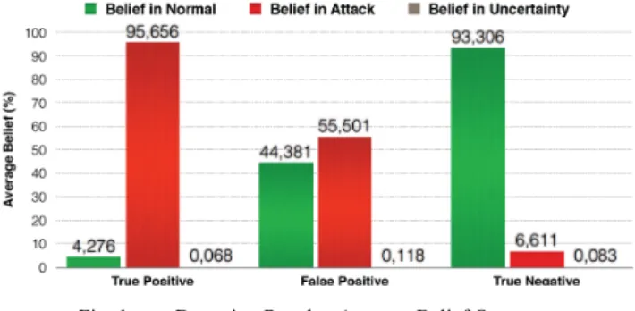
Fig. 1. Detection Results: Average Belief Outcome.
The detection results were analysed to confirm that the different beliefs were consistent with what was expected. As can be seen in Fig. 1, the correct detection is produced by very strong beliefs in the appropriate hypothesis. In the cases of TP results, the average belief in Attack is 95.66%. In the case of TN results, the average belief in Normal is 93.3%. This gives strong reasons to trust the IDS, and in turn, trust that the different instances from the original dataset could be labelled according to the final results of the IDS. Another encouraging factor about the results is that none of the malicious instances were misclassified as non-malicious. No FN were generated.
Different beliefs behaviour can be seen in the cases of FPs. In the cases in which none of the belief results provides strong support to one of the hypotheses, the non-malicious instances have been misclassified as malicious. The average belief in
Normal is 44.38%, and the average belief in Attack is 55.5%
for these frames. The ambiguous beliefs make the detection system produce erroneous results. This is a drawback for the idea of labelling the different instances of the original dataset simply according to the outcome of the detection system. The following section tackles this issue.
D. Beliefs Difference Results Analysis
The principal aim of this work is to propose a methodology to produce automatically labelled datasets. A possible solution, similar to the one proposed in [4], could be to use an existing, unsupervised anomaly based IDS as an automatic anomaly classifier, i.e. the one proposed in [7], to label the instances datasets according to these results. If it was assumed that strong belief results of the detection system were completely accurate, each instance in the original dataset could be labelled according to the decision results. However, it has been proved that this is not the case. False alarms do occur as shown below.
From the detection results presented in the previous section, it can be understood that the actual difference between the belief in Normal and the belief in Attack plays an important role in the correct detection of the attacks. Therefore, if an appropriate threshold defining the boundary between strong and weak belief results could be found, misclassified instances could be discarded from the automatically labelled dataset. The instances with differences above this threshold would be included in the labelled dataset, whereas the instances with belief results differences below this threshold would not be included. The difficulty here is to find the right mechanism to automatically define the appropriate threshold.
Fig. 2. Histogram and Boxplot - Beliefs Difference of Original Dataset, using Normal and Malicous Instances.
In order to have a clearer idea of how the belief results are distributed, an analysis of these results is presented. Fig. 2 (a) shows a histogram that represents the frequency of the beliefs difference for all the instances in the original dataset, and Fig. 2 (b) the boxplot that represents the distribution of the beliefs difference, using the actual nature of the frames as the distinction criteria. Although these are different methods, both are different representations of the same dataset values. Graphically, the results in Fig. 2 (b) show that there is no evident distinction between the distribution of the belief difference results for malicious and non-malicious information.
The mean of the differences for the whole dataset is µtotal = 0.8694, and the standard deviation is σtotal = 0.1125. This dataset includes both malicious and non-malicious instances. Considering only non-malicious information, 13418 instances, the mean value of the frequency of the beliefs difference is µnormal = 0.866, and the standard deviation is σnormal = 0.1152. Considering only malicious information, 995 instances, the mean value of the frequency of the belief difference is µattack = 0.914, and the standard deviation is σattack = 0.0445.
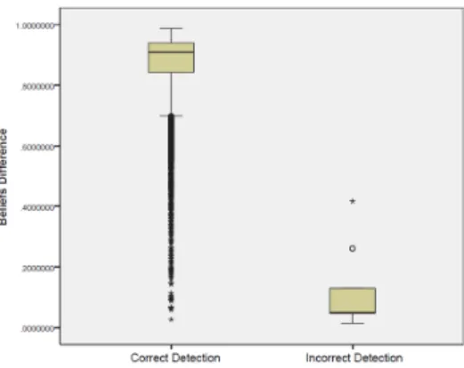
Fig. 3. Beliefs Difference - Correctly and Incorrectly Classified Instances.
Fig. 3 shows another boxplot that represents the distribution of the beliefs difference. In this case, classification results assigned by the unsupervised anomaly based IDS to the frames are used as the distinction criteria. This is whether the frames are correctly or incorrectly classified instances in the dataset. Considering only correctly classified information, 14398 instances, the mean value of the frequency of the beliefs difference is µcorrect = 0.8702, and the standard deviation is σcorrect = 0.1098. Considering only incorrectly classified information, 15 instances, the mean value of the frequency of the belief difference is µincorrect = 0.1112, and the standard deviation is σincorrect = 0.1154. In contrast to the previous representation of the belief difference results, there is a very clear distinction in the difference values between the correctly classified and the incorrectly classified instances.
E. Automatic Dataset Labelling Methodology
The methodology that has been used in this work to define the boundary threshold is based on the mean (µ) and standard deviation (σ) values. In the histogram presented in Fig. 2, the distribution of the belief difference results follows an asymmetric Normal distribution. The coefficient of Skewness value -2.706 and the Kurtosis value 10.488 prove the negative asymmetric skewed distribution. Using the properties of this distribution, the boundary threshold (γ) could be defined by (1). The definition of (1) as the threshold γ has been empirically defined. However, based on the statistical theory, (1) ensures that the labelled dataset will contain about 95.44% of the original dataset and, at the same time, it will assure that only correctly labelled instances are included in the new dataset.
First, the wireless network traffic is gathered to create the original dataset. For each frame in the dataset, the IDS provides three belief values, based on the data. Each frame is initially labelled according to the belief with the highest value. Then, for each instance, the difference between the belief in Normal
and Attack is calculated. Next, the µtotal and σtotal of the beliefs
difference is calculated and the γ is calculated. Finally, each
frame for which the belief difference is larger than γ is kept in the labelled dataset. Otherwise, the frame is removed from the labelled dataset. Using (1) over the actual values µtotal and σtotal of the original dataset, the boundary threshold value would be γ
= 0.8694 – (2×0.1125) = 0.6444. For this dataset, any instance where the difference between the belief in Normal and Attack is larger than 0.6444 will be included in the labelled dataset. In contrast, any instance where the difference between the belief
in Normal and Attack is smaller than 0.6444 will be discarded.
γ = µtotal - 2σtotal (1)
The results obtained after filtering the information using the boundary threshold are presented in Fig. 4. This histogram represents the frequency of the beliefs difference only for the instances in the original dataset that satisfy the boundary threshold condition. For this new dataset, a subset of the original dataset, the mean of the differences is µ = 0.8883, and the standard deviation is σ = 0.071. For these values, the coefficient of Skewness is -1.309 and the Kurtosis is 1.138. In total, 13702 instances, both malicious and non-malicious, compose the new labelled dataset. This is, as expected, 95.067% of the original dataset. All the incorrectly labelled instances have been discarded, as well as 696 correctly labelled instances. Nonetheless, this is a small number of instances, compared with the 13702 instances considered. This new correctly labelled dataset, composed of non-simulated IEEE 802.11 frames captured from a real WiFi network, could be used to train supervised IDSs, or processed by a feature selection approach.
Fig. 4. Histogram - Beliefs Difference of New Automatically Labelled Dataset, using Normal and Malicous Instances.
As a recap, the process of gathering the wireless network traffic, the detection process, the generation of the new training dataset and the labelling process, are all implemented automatically and autonomously by the proposed system, without the mediation of any human administrator. In addition, both the training process of the supervised IDSs [4] and, as explained in Section IV, the selection of metrics could also be implemented automatically. In addition, the small subset of discarded instances could be manually classified and added to the automatically labelled dataset if required to ensure a consistent dataset. The manual effort required to do this would be much reduced. This approach enhances the capabilities of IDSs deployed in commercial, private and tactical network infrastructures by streamlining the process and reducing the cost for the need of an administrator.
IV. FEATURE SELECTION
Feature Selection refers to a group of techniques able to minimise the number of metrics in a given dataset and optimise the selection process of the most relevant set of metrics [2]. In the field of intrusion detection, these techniques play an important role in improving the efficiency of the IDSs, detecting the maximum number of attacks and producing the minimum number of false alarms. In [9], the authors show the benefit of feature selection techniques to improve the overall detection accuracy of their system. Ideally, all IDSs should implement feature selection as part of their framework to improve the attack detection accuracy.
Nonetheless, the implementation of automatic feature selection techniques for unsupervised IDSs is still a great challenge for researchers in intrusion detection [3], especially if the IDSs perform the detection in real-time. One of the reasons is because feature selection works only if the datasets have been previously labelled [3]. Feature selection requires labelled datasets to be able to evaluate the relevance of each metric or combination of metrics.
In our previous work [7], six metrics were experimentally selected after manual off-line analysis, as the most appropriate metrics for detecting the attacks. If appropriately analysed, the IDS can identify all the different attacks that we implemented. In this work, feature selection techniques have been employed to select the most appropriate set of metrics, using the automatically labelled dataset, from amongst all the six metrics. A Genetic Algorithm (GA) based approach has been employed to implement the feature selection tasks. The GA will automatically provide the most appropriate set of metrics, for each analysed dataset. Whilst six metrics does not entail high computational demand to the feature selection technique, and the metric selection could be done through exhaustive search, the GA could reduce the computational demand in situations in which a greater number of metrics is considered.
A. Genetic Algorithm
A GA is a stochastic search technique to find the optimum solution for an optimisation problem. It is a general technique that could be applied in many research areas [8]. It is particularly useful where other application techniques are not appropriate. An example would be where the search space was too large for exhaustive analysis.
A GA uses the concept of chromosomes. A chromosome is a binary representation of solution vectors, a fixed length array with sequences of bits {0, 1}. In our system, each slot of the array represents one of the considered metrics. 1's mean that the metric is included, and 0's mean that the metric is discarded. The chromosomes evolve through successive iterations or generations. It is expected that after successive generations, the chromosomes with higher fitness function value (ffitness) prosper while those with lower ffitness disappear [8]. It is important to empathise that, since this is a stochastic technique, successive experiments of the GA over the same dataset will not always produce similar final results. The ffitness is a quality measurement that indicates how well each individual chromosome fits the design requirements.
Before starting the process, the GA requires the specification of certain parameters. For our system, these are the Initial Population Size (n), Chromosome Length (l),
Number of Repetitions (r), Crossover Probability (PC) and Mutation Probability (PM). The value l = 8 is established by the number of metrics, 6, and 2 additional parameters that compose the chromosome. The first six slots are the representation of the six different metrics. The 7th slot in the chromosome is the decimal indexation of the selected metrics, used only for evaluation purposes. The 8th slot is the f
fitness for the particular selection of metrics. The PC commonly ranges between 0.6 and 0.95, and the PM ranges between 0.001 and 0.01, according to [13]. In our experiments PC = 0.7, PM = 0.01 and n = 6 have been empirically chosen. These parameters were kept unchanged during the experiments.
A GA follows a 6-steps process. In the first step, Initialisation, the GA randomly selects the initial population of n chromosomes. This is a subset of all the available chromosomes. Next, in the Evaluation step, the ffitness for each chromosome in the initial population is calculated. In the third step, Selection, the ffitness is used to select the chromosomes that will become parents for the next generation of chromosomes. Among other selection techniques that have been proposed in the literature, the Roulette Wheel has been applied in this work, due to its simplicity and good performance. The roulette wheel gives a biased weight to each of the selected chromosomes, based on the ffitness [8]. The chromosome with better ffitness has a higher probability of being selected. In the forth step, Crossover, it is decided if a pair of chromosomes mate, with probability PC, to produce a new pair of chromosomes. Using the One Point Crossover method, a number between 1 and l is randomly chosen, which defines the Crossover Point (Cp). The new pair is generated by leaving unmodified the portion of the chromosomes from the first bit to the Cp and interchanging the portion from the Cp to the last bit of the chromosomes. If the chromosomes do not mate, these remain unmodified. The last step, Mutation, adds random modifications to the new population of chromosomes to provide some level of diversity. With PM, one of the bits that comprise each chromosome will be reversed from 0 to 1, and vice versa. The process is repeated r times, from the 2nd to the last step.
B. Genetic Algorithm Experiments and Results
A diverse set of experiments has been conducted to evaluate the capability of the implemented GA based approach. The experiments evaluate the effect of changing some of the GA parameters in the final metric selection results. In particular, we focused on varying r and the ffitness. The value of
r would have a direct effect on the time and computational cost to implement the GA process. The larger this value, the higher the cost, but a value of r that was too small might influence the metrics selection. A small value of r would not allow the GA to converge to a particular result.
Initially, a succession of 50 GA experiments were carried out with r = 500, using both the original dataset and the new automatically labelled dataset. The original dataset was manually labelled through an exhaustive off-line forensic analysis for these experiments. The used ffitness, defined by (2), is based on the DR and FPr. One particular set of metrics was selected as the final result for each GA experiment.
For the 50 experiments with the original dataset, the GA converged to the final result, on average, at the 369th repetition. Not all the resulting sets of metrics produced 100% DR and 0%
FPr. Through all the experiments with the original dataset, the results with highest DR and lowest FPr would have been produced, on average, at the 194th repetition. For r = 500, 369 and 194, the average DR(%) results are 99.79, 99.65 and 99.11, whereas the average FPr(%) results are 0.91, 1.96 and 1.74, respectively. For the 50 experiments with the new dataset, the GA converged to the final result at the 355th repetition, on average. For this dataset using (2), the results with highest DR and lowest FPr would have been produced, on average, at the 155th repetition. For r = 500, 355 and 145, the average DR(%) results are 99.4, 99.66 and 99.44, whereas the average FPr(%) results are 1.38, 2.07 and 2.73, respectively. Comparing the results from these experiments show that the value of r does not have a major impact on the results performance of the GA.
ffitness = DR + (100–FPr) (2)
ffitness = DR + (100–FPr) + (MetricsTotal–MetricsSelected) (3) The set of metrics selected in the different experiment has not always produced perfect detection. Only 18% of the 50 experiments provided perfect detection with the original dataset, whereas 46% of the 50 experiments provided perfect detection with the new dataset, using the same ffitness, (2). These results also show an overall improvement in the selection of metrics by using the automatically labelled dataset instead of the manually labelled original dataset. This is because the automatically labelled dataset does not contain doubtful data, which reduce the overall risk of FP and increase the DR.
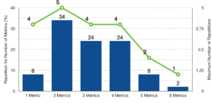
By using an alternative ffitness it was intended to identify a set of metrics that effectively produce 100% DR and 0% FPr. In addition, obtaining these results with the fewest number of metrics would be also beneficial for the IDS. The ffitness in (3) is based on the DR, FPr and the total number of metrics. Also, two conditions were added, where DR = 0 if DR < 100% and FPr = 100 if FPr > 0%. By using (3) with the new dataset, all the resulting sets of metrics produce 100% of DR and 0% of FPr, as expected. Represented in Fig. 5, for the 50 experiments, sets of metrics with 1 metric have been selected 8% of the time; 2 metrics 34%; 3 metrics 24%; 4 metrics 24%; 5 metrics 8%; and 6 metrics only 2% of the time. If we focus on the number of times each set of metrics is selected, the set with 1 metric that is selected more frequently, 4 times, is Rate; the set with 2 metrics that is selected more frequently, 5 times, is Rate-TTL; with 3 metrics is Rate-TTL-ΔTime, 4 times; with 4 metrics is RSSI-Rate-TTL-NAV, 4 times; with 5 metrics is RSSI-Rate-TTL-NAV-SEQ; and the set with 6 metrics is selected only 1 time. These results are represented in Fig. 5.
V. CONCLUSIONS
This paper tackles the automatic generation of labelled real network traffic datasets, and the automatic selection of metrics. IDSs deployed in commercial, private and tactical network infrastructures may benefits from the developed approach. This approach labels datasets according to the results of an unsupervised IDS. We use the outcome beliefs of the IDS and consider correct only the cases in which the beliefs difference evidences strong support to one of the hypotheses. This approach filters out doubtful results and reduces the risk of misclassification. The new dataset is a subset of the original dataset. As the remaining portion of the dataset might contain valuable information, it would be feasible for the system
administrator to manually classify and add these instances to the automatically labelled dataset to ensure a consistent dataset. It is seen that, using a GA, it has been possible to implement an automate feature selection approach using the labelled dataset. It has been experimentally proven that the number of repetitions does not have major impact on the final results. In the GA, the ffitness plays the most important role in the implementation of this technique. The ffitness allows the GA outcomes to be fine tuned, whether this is maximising the DR, minimising FPr, number of metrics, or some other parameter.
Fig. 5. Bar Chart of the Resulting Set of Metrics Frequency
REFERENCES
[1] P. Laskov, P. Düssel, C. Schäfer, and K. Rieck, “Learning intrusion detection: supervised or unsupervised?,” in Image Analysis and Processing-2005. vol.3617, Springer Berlin Heidelberg, 2005, pp. 50-57. [2] G. Stein, B. Chen, A. S. Wu, and K. A. Hua, “Decision tree classifier for network intrusion detection with GA-based feature selection,” Proceedings of the 43rd annual Southeast regional conference-Volume 2. ACM, 2005, pp. 136-141.
[3] H. Nguyen, K. Franke, and S. Petrovic, “Improving effectiveness of intrusion detection by correlation feature selection,” Proceedings of the IEEE International Conference on Availability, Reliability, and Security,
ARES'10, 2010, pp. 17-24.
[4] F. Gargiulo, C. Mazzariello, and C. Sansone, “Automatically building datasets of labeled IP traffic traces: A self-training approach,” Applied Soft Computing 12.6, 2012, pp. 1640-1649.
[5] OPNET Modeler, Available: http://www.riverbed.com/products-solution s/products/opnet.html?redirect=opnet (Access Date: 14 Apr, 2014). [6] E. Eskin, A. Arnold, M. Prerau, L. Portnoy, and S. Stolfo, “A geometric
framework for unsupervised anomaly detection,” Applications of data mining in computer security. Springer US, 2002, pp. 77-101.
[7] F. J. Aparicio-Navarro, K. G. Kyriakopoulos, and D. J. Parish, “An automatic and self-adaptive multi-layer data fusion system for WiFi attack detection,” International Journal of Internet Technology and Secured Transactions 5.1, 2013, pp. 42-62.
[8] J. Fan, PhD Thesis, “Using genetic algorithms to optimise Wireless Sensor Network Design,” Loughborough University, 2009.
[9] C. Dartigue, H. I. Jang, and W. Zeng, “A new data-mining based approach for network intrusion detection,” Proceedings of the IEEE Seventh Annual Communication Networks and Services Research Conference, CNSR'09, 2009, pp. 372-377.
[10] C. A. Catania, and C. García Garino, “Automatic network intrusion detection: Current techniques and open issues,” Computers & Electrical Engineering 38.5, 2012, pp. 1062-1072.
[11] J. J. Davis, and A. J. Clark, “Data preprocessing for anomaly based network intrusion detection: A review,” Computers & Security 30.6, 2011, pp. 353-375.
[12] Airpwn, Available: http://airpwn.sourceforge.net/Airpwn.html (Access Date: 14 Apr, 2014).
[13] Y. J. Cao, and Q. H. Wu, “Teaching genetic algorithm using MATLAB,” International journal of electrical engineering education 36.2, 1999, pp. 139-153.