Enhancing the SVDD Accuracy in Intrusion Detection Systems by removing
External Voids
Tayeb Kenaza†, Khadidja Bennaceur†, Abennour Labed†, Mahdi Aiash‡ †Ecole Militaire Polytechnique
PB 17, Bordj El Bahri, Algiers, Algeria
Email:{ken.tayeb,khadidja.bennaceur.19,a-labed}@gmail.com ‡Scool of Science and Technology, Middelsex Univesity, UK
Email: [email protected]
Abstract—This work aims to improve the accuracy of the SVDD-based Intrusion Detection Systems. In this study we are interested by approaches using only one-class classification, namely the class of normal user sessions. Sessions are modeled by vectors of points in a finite features space. The goal of using the SVDD in anomaly detection is to find the hypersphere with a minimal volume that encloses the entire scatter of points (i.e. the normal sessions). This paper discusses the general case where the shape of the scatter is arbitrary. In this case some voids can occur between the scatter and the boundary of the hypersphere, and mainly cause a distortion of the data description that reduces the accuracy of the detection. The objective of this work is to study and highlight the best techniques that help removing voids and thus improving the ac-curacy of the SVDD. Experimental results show that choosing the appropriate techniques and parameters can significantly improve the accuracy of the SVDD.
1. Introduction
The last decade has seen a remarkable Internet develop-ment, characterized by the increasing speed, the power of the available infrastructure, and the reliability of services delivered to users. However, this development has been accompanied by an increasing number of threats and cyber-attacks. Intrusion Detection Systems (IDS) are hardware or software solutions that automatically detect intrusions. They, mainly, run in two modes: (i) The detection of signatures of known attacks. (ii) The detection of sessions outside the normal behavior (also called anomaly detection). In [11], authors review most of recent works on intrusion detection. In this work we are interested by the network anomaly detection. Several methods have been proposed in this do-main. In [21], authors propose a classification of methods that detect anomalies on networks. Generally, recent meth-ods are of two types: (i) Detection methmeth-ods based on binary classification that determines a boundary between positive objects that represent the legitimate sessions and negative objects that represent intrusive sessions. The most used binary classification method is the Support Vector Machine (SVM) [5] [17] [16]. (ii) Detection methods based on
one-class one-classification or data description which is a specific kind of multi-class classification, where there is a single target class of only positive objects, for which a boundary is constructed.
The one-class classification method studied in the present paper is the Supports Vectors Data Description (SVDD) [18]. It aims at finding the minimal hypersphere (with minimal radius) that encloses the entire training dataset. The SVDD and its variants have many applications such as, anomaly detection in the measurements of the temperature and pressure in gas pipelines [14]. In [13] authors use the SVDD in the detection of the sudden change of engine temperature in hybrid electric vehicles. The SVDD is also used in intrusion detection. In [10], authors propose to solve the ambiguity problem, in case of points that are close to the hypersphere boundary. They make a clustering at these points by the K-means and then they reallocate these clusters either within or outside the hypersphere. Another variant of the SVDD based on uncertainty is proposed in [12]; authors add to each object a confidence factor then they adapt the training with a generalized SVDD.
In practice, having a scatter with a perfectly spherical shape is very rare. So, in most cases, this type of modeling leads to a hypersphere containing voids (very low-density areas compared to the neighboring) which are external, when they come in contact with the boundary of the hypersphere. Voids may also be internal, when they are surrounded by points with a high-density. In this case, the SVDD misrep-resents the training set because voids increase the number of false negatives. In [9], an approach based on finding the largest void has been proposed to formally evaluate a one-class one-classifier.
In this paper, we study and highlight methods that aim to eliminate external voids in order to reduce the number of false negatives and, therefore improve the detection ac-curacy. First, the SVDD is tested with two types of kernels: polynomial and Gaussian. Then some data preprocessing techniques are used prior to the learning step. This pre-processing consists to features scaling. Finally, in order to improve the accuracy in the case of polynomial kernel, we propose to use another preprocessing before the features scaling, namely a data centering.
This paper is organized as follows: In section 2 a theoret-ical presentation of the SVDD is given. Section 3 discusses methods used for removing voids. Section 4 presents an em-pirical study and a comparison between discussed methods. Section 5 concludes the study.
2. Support Vector Data Description (SVDD)
The SVDD is a one-class classification method, similar to the conventional binary classification, except that instead of having to distinguish between two different classes, one has to decide whether an object belongs or not to a dominant class of objects called “Target class”. Objects that do not belong to the target class are called “Outliers”. It is worth mentioning that if the training set does not contain a suf-ficient number of attack samples, the binary classification becomes inadequate, and a one-class classification based on the description of the boundary of the training set is required.
Moreover, the SVDD can be used as a multi-class clas-sifier. In [19], authors propose to split the target class into sub-groups; each one is bounded by an SVDD. An other approach based on binary classification is proposed in [15]; where both the target class and the outliers are enclosed in two different hyperspheres.
The SVDD method is inspired by the support vector machine (SVM) [3]. Recall that the SVM technique tries to find a hyper-plan that separates at the most two classes, while the SVDD tries to find a hypersphere with minimum radius that encloses all the training set. This hypersphere is characterized by the centeraand the radiusR. Mathemati-cally, this can be resolved by minimizing the cost function:
F(a, R) =R2 (1) under the condition that the distance between each point and the center is less than or equal to the radiusR:
kxi−ak ≤R2(i= 1, ...N) (2) To solve this nonlinear constrained optimization prob-lem, the Lagrangian is introduced:
L(a, R, αi) =R2− N
X
i=1
αi(R2− kxi−ak2) (3)
where the αi≥0 are the Lagrange multipliers.
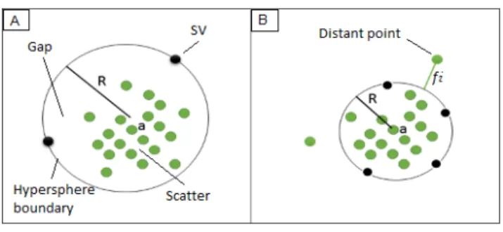
Only few αi are not null, therefore only a few objects of the training set are involved in the determination of the hypersphere. These objects fall on the boundary of the hypersphere and are called Support Vectors (SVs) (figure 1-A). After calculating SVs, the center is easily determined. Indeed, we simply cancel the partial derivative of the La-grangian with respect to a.
δL/δa= 0⇒a=xi N
X
i=1
αi (4)
The radiusRis the distance between the center and any of the support vectors. The identification of the center a
and the radiusRfrom the training set, provides the learning model that can be used to check if an object belongs or not to the description. If the distance between an object and the centera, is less thanR, it is accepted and considered as an object of the target class.
kz−ak2≤R2 (5) However, if the distance from the object to the center is higher than R, it is rejected and considered as an Outlier. It should be mentioned that the model of the sphere is too simplistic. In practice, the scatter of points representing the training set is never perfectly spherical. Therefore, there will always be voids between the scatter of point and the contour of the hypersphere. So, in order to obtain an accurate model, this problem of external voids deserves a particular attention. A first solution to this problem has been proposed by Tax [18], which is inspired by the work proposed in [3].
3. Voids removal
3.1. Elimination of distant points
This solution is recommended when the training set con-tains some objects that are distant from the whole set (Figure 1-B). In this case, we obtain a hypersphere relatively large, which miss-describes the scatter of points (several external voids occur inside the hypersphere). So, it is suggested to reject these points before the training. This allows reducing voids in the hypersphere. Theoretically, each point xi is assigned a variable fi. Then, the cost function given by (1) becomes: F(a, R) =R2+C N X i=1 fi (6)
under the conditions:
kxi−ak2≤R2+fi and,
fi≥0
(7)
C is a constant called regularization parameter.
Figure 1. SVDD hypersphere
Voids elimination reduces the number of false negatives. However, rejection of distant points increases also the num-ber of false positives. The parameterC, fixed by the user, allows making compromise between these two situations.
The Lagrangian associated with the optimization problem becomes: L(a, R, fi, αi, γi) = R2 + CP N i=1fi − PN i=1αi(R2+fi− kxi−ak2)−P N i=1γifi (8) Now, canceling the partial derivative of the Lagrangian with respect to aandRleads to:
L= N X i=1 αi(xi.xj)− N X i=1 αiαj(xi.xj) (9)
under the constraint 0 ≤ αi ≤C and C > 1/N. The expression of the centera remains unchanged.
The major difficulty with this solution rely to the choice of the parameter C. It depends on the shape and the distribution of the scatter of points. This solution is most effective when the scatter is more spherical and contains just a few points that are distant from the majority. However, it becomes less effective if the scatter is spread with respect to one of feature space dimensions (Axis). In this case, the distant points could not be avoided. An other solution that takes into account the real shape of the scatter is explained in section 3.2.
An opposing approach is detailed in [20]; instead of eliminating distant objects, authors eliminate objects located in high density area. Then, only points that fall on the hypersphere boundary are used in the training. This solution does not decrease the accuracy but reduces the learning time.
3.2. Kernel function
The introduction of a kernel function is used to learn the spherical shape of the SVDD more flexibility. Implicitly, through a functionF, this approach consists to represent the point’s xi into another space of feature with their images
F(xi) and the training is applied to this new space of feature. Different functionsF mean different new represen-tations of the scatter and thus different learning models. The best function is the one that represents the training set in a spherical shape and keep outside the Outliers. Mathemat-ically, everything is done by replacing the inner product
(xi.xj)in 9 by the functionK(xi, xj) =F(xi).F(xj). The literature provides different kernel functions, but the choice of an appropriate kernel function depends on the dataset, and only tests helps identifying the best function and the best value of parameters to use for a given dataset. In the following, we will limit our study to the presentation of two families of frequently used functions.
3.2.1. Gaussian kernel. The Gaussian kernel function
also called Radial Basis Function (RBF) is defined by
K(xi, xj) = exp[− kxi−xj k2 /s2]. This function does not depend on the positions of pointsxiandxj, but depends on the Euclidean distance kxi−xjk between these points. This function is often chosen because it allows reducing the dominance of the farthest points in the construction of the learning model. s is a parameter fixed by the user. By varying s, the whole model varies. We can have a scenario
between two extremes cases: (i) The over-training where all points are support vectors and (ii) The standard SVDD model (perfect hypersphere). The practical difficulty of this function is the determination of the optimal value of the parameters for a given dataset. Some works was carried out to propose methods of estimation of an optimal value for parameters that provide the best accuracy rate. In [14], authors propose an heuristic to estimate the optimal value ofs, depending on the training set. Also, they have changed the expression of the Gaussian kernel using different type of distances. An intermediate approach between the rigidity of the hypersphere and the flexibility offered by the Gaussian kernel was proposed in [7]; this approach is based on searching for the minimum hyperellipsoid that encloses all the training set. This is more effective in the case of an extended scatter of points; it helps to follow the shape of the scatter without crossing the problem of choosing the parameters.
3.2.2. Polynomial kernel. The expression of this function
is: K(xi, xj) = (1 + xi.xj)d, d is the degree of the polynomial.
This function transforms the scatter of points corre-sponding to the training set from the original feature space to another feature space of higher dimension, where an object is represented by the original features and all the products of these features up to degreed. For instance, in the case of a vector space with two featuresxi(xi1, xi2)andxj(xj1, xj2), the formula of the polynomial kernel of degreed= 2is:
K(xi, xj) = [(xi1xi2)(xj1xj2)T + 1]2 (10) After development we obtain:
K(xi, xj) = (xi1)2.(xj1)2 + (xi2)2.(xj2)2 +
2(xi1.xj1)(xi2.xj2) + 2(xi1.xj1) + 2(xi2.xj2) + 1 (11) So, each point is represented in a new space with five dimensions which are:x2
1,x22,x1.x2,x1 andx2.
Clearly, unlike the Gaussian kernel, this function de-pends on the positions of the point’s xi in the space, regarding the reference center. Indeed, the value of the radius
R varies according to xi and the degree d. Choosing a high degree d, generates a poor description if it contains some points xi that are too far from the origin; it lead to a large value of R. Moreover, the dimension of the new space increases exponentially and requires more memory resources for data storage.
3.3. Feature scaling
The feature scaling of a scatter points consists in chang-ing the shape of the scatter accordchang-ing to the distance ratio between points on each dimension. The feature scaling is required if there is a significant discard between points in one or more dimensions (i.e. the scatter is stretched over some dimensions). It aims to reduce the distances between the points and put them on similar scale. In [6], the author classified the one-class classifiers into two types: a type
that is not sensitive to the scaling, i.e. the accuracy of the classifier does not vary by applying a features scaling such as the Principal Components Analysis (PCA). The second type of classifiers is sensitive to scaling such as the k-means, k-nn and SVDD; because these classifiers depend on the shape of the scatter. In the case of SVDD, more the shape of the scatter is spherical, more the hypersphere describes best the scatter (less external voids) and the accuracy rate becomes higher. In [18], Tax provided a first method of feature scaling, it is the scaling using the variance. Then, in [8], authors has presented another two methods: one using domain and the other using min-max.
1) Scaling using the variance: each value xlm of the
lth feature is divided by the variance the feature setσl. In case where the points on a dimension are spread; therefore, this helps to bring all the values
xlm on the same scale.
2) Scaling using the max: each value xlm of thelth feature is divided by the maximal value the feature set (maxl); thus, all the feature values will belong to the interval[0,1].
3) Scaling using the min-max: each valuexlm of the
lth feature is divided by the minimal value of the maximums of all features. All feature values will belong to the interval [0, R], where R is the min-max.
The feature scaling has a practical advantage. Searching the spherical shape on another space, by using a kernel function, lead to the problem of choosing the appropriate kernel function and its parameters. It is better to transform, in the original space, the scatter into a more spherical shape. However, the disadvantage is that it treats each feature sep-arately, whereas in reality, features are often interdependent, which may break this interdependence and induces a loss of precision.
3.4. Data centering
Regarding the polynomial kernel function K(xi, xj) =
(1 +xi.xi)d, we recall that this function is strongly relied to the values of xi. Thus, if the scatter contains some points xi that are too far from the origin O, this would lead to a relatively large hypersphere and therefore to a bad description. In SVDD, what is important is not the position of the points relatively to the center, but the shape of the scatter and the distances between points. The idea is to conserve the distance between points and make translation of the origin O to the center of gravity of the scatter. On each dimensionl, the coordinate of the new originO0, will be:
O0l= (maxl+minl)/2
Wheremaxlandminlare , the maximum and minimum values on the feature l, respectively. In this way, the points are said to be balanced around the center. This reduces the feature values; and therefore, the minimum value of the radiusR.
4. Experiment
Before starting tests we have chosen and formated a benchmark as needed. The details are given below.
4.1. Benchmark preprocessing
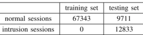
The tests are performed on the KDD99 benchmark. It consists of a set of sessions labeled by normal or attack. Each session is characterized by 42 features. Therefore, each session may be represented by a vector of 42 coordinates. Since this work is concerned by the one-class classification, it is limited to only normal sessions. In [4], authors detail the benchmark preprocessing steps to apply before starting the test phase. Table (1) shows the size of the training set and the testing set. In this work the library LIBSVM [2] is used in the learning step.
TABLE 1.BENCHMARK OF TEST training set testing set normal sessions 67343 9711 intrusion sessions 0 12833
Features type transformation
Recall that the 42 features of this benchmark are of three types: decimal features (continuous), Binary features (0 or1) or Nominal features (they take values from a finite list). For example, the feature Protocol can be (TCP, UDP, ICMP). There is no logical order between the elements of this list. The SVDD is an oriented distance method. It must calculate the distance between points. We have, for example, two points xi and xj, calculating the distance kxil−xjlk following the dimensionl is trivial in the case wherel is a decimal feature. If the feature is binary, this distance is zero whenxil andxjl are both equal to1or 0; or it is equal to 1 when xil differs from xjl (i.e. xil > xjl or xil < xjl). So, the order betweenxi andxj is not important.
Nominal features need to be converted before calcu-lating the distance. The conversion can be done using a method based on classification trees [1]. It converts each nominal feature A withN possible values (val1, ..., valn) to N binary features, where the ith feature is “A=vali”. For example, the features “Protocol”= (TCP, UDP, ICMP) in converted to three binary features “Protocol = TCP”, “Protocol = UDP”and “Protocol = ICMP”. If the protocol is “TPC”, the feature “Protocol = TCP”is set to1and all others are0. In this way, nominal features are transformed to binary features which allows calculation of the distances without having to establish an order between the values of features. On the KDD99 benchmark, this conversion increases the number of feature from 42 to 122, so it adds 80 additional binary features. There are some features that all values are equal to 0, for example: no sessions is under the protocol “ICMP” then the new feature “Protocol = ICMP”is always equal to 0. These features were eliminated because they
do not contribute to distinguish between points and also to avoid computational problems (division by zero).
4.2. Test of kernel SVDD
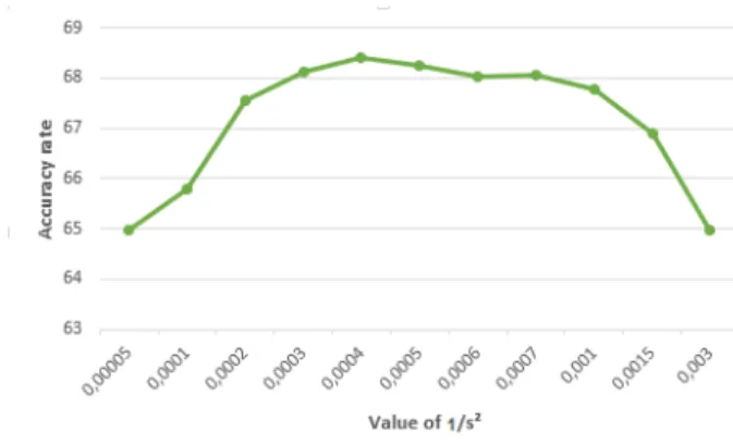
The test of the standard SVDD presents an accuracy rate of 61%. The results of the test of SVDD with polynomial kernel by varying the degreedand the tests of SVDD with Gaussian kernel by varying the parameter s are shown in Figures 2 and 3, respectively.
Figure 2. Accuracy of polynomial kernel SVDD w.r.t. degreed
The best results are obtained for the degree d= 2 and
d = 3, then more we increase the value of d, more the accuracy decreases. When, a value of the degreedis greater than 4, the number of the feature in the new space becomes enormous. We note that for the three values considered tod, the results provided by the SVDD with polynomial kernel are always better than that provided by standard SVDD.
Figure 3. Accuracy of the Gaussian kernel SVDD w.r.t.1/s2 Figure 3 shows that the best accuracy is obtained when the value of 1/s is between 0.0003 and 0.0007. Note that the SVDD with polynomial kernel gives slightly better results than the SVDD with Gaussian kernel. This is due to the default position of the point scatter produced by the KDD99 benchmark. But the results from this SVDD are always better than the standard SVDD.
4.3. Test of the feature scaling
We tested three standard scalling before learning with the standard SVDD and SVDD with kernel function ( Gaus-sian and polynomial). The best scores are in the table 2.
TABLE 2. RESULTS OF THE FEATURE SCALING
Without scaling Variance Domain Minmax
SVDD 61 71 82 61
SVDD+Gaussian 68 70 83 68 SVDD+Polynomial 70 67 79 70
The results summarized in table 2 illustrate that the scaling by min-max did not improve the results because of the existence of binary features where the maximum is equal to1, wich is also the minimum of the maximums of all features. So the scaling (division by1) does not change the feature values and therefore it has no influence on the model.
In the case of scaling by the variance, there is an improvement of10% for the standard SVDD. A slight im-provement is obtained by using the Gaussian kernel, because this way of scaling practically plays the same role as the Gaussian kernel. The latter reduce the dominance of the farthest points, and scaling by variance reduces distances between the points and thus brings distant points.
The best results are obtained by applying the scaling by domain. The standard SVDD and the SVDD with Gaussian kernel give almost the same score of about82%due to the dominance of binary features (over than 80 binary features), where default values are between0 and1
4.4. Test of data centering
Data are centred before the scaling step. The results obtained are shown in Table 3.
TABLE 3. DATA CENTERING RESULTS
Scaling (domaine) Centring + Scaling (domaine)
SVDD 82 71
SVDD+Gaussian 83 83
SVDD+Polynomial 79 d=2 d=3 d=4 82.94 83.62 83.67
Following this preprocessing (scaling + centering), when we increase the value of the degree d , the accuracy of the learning with SVDD and polynomial kernel don’t de-crease like in the case without preprocessing; However, we found a slight improvement. We note that the SVDD with polynomial kernel is improved to be at the same level of performance as the standard SVDD and SVDD with Gaussian kernel. Therefore, it is obvious that it would be interesting to learn with the standard SVDD (simple model); and deal with the problem of choosing the appropriate kernel function and its parameters.
5. Conclusion
In this paper, the performance of intrusion detection systems based on the SVDD method is tested using two types of kernel functions, namely polynomial and Gaussian. Both Kernel functions give a better score than the standard SVDD. However, the most appropriate function as well as its parameters can only be fixed experimentally, i.e. after having the test results.
Then, a feature scaling technique is applied as a prepro-cessing. As a result, we obtain an improvement in all tested models, namely the standard SVDD, SVDD with Gaussian kernel, and SVDD with polynomial kernel. But the latter remains less powerful than the other. This is rectified by applying another preprocessing, namely the data centering which consists to moving the origin of the features spaces to the gravity center of the scatter.
Therefore, after getting three scores (of the three models) almost equal, we can say that the feature scaling and the data centering allow to overcome the hard problem of choosing the appropriate kernel function and its parameters.
References
[1] Leo Breiman, Jerome Friedman, Charles J Stone, and Richard A Olshen. Classification and regression trees. CRC press, 1984. [2] Wei-Cheng Chang, Ching-Pei Lee, and Chih-Jen Lin. A revisit to
support vector data description (svdd). Technical report, Citeseer, 2013.
[3] Corinna Cortes and Vladimir Vapnik. Support-vector networks.
Machine learning, 20(3):273–297, 1995.
[4] Jonathan J Davis and Andrew J Clark. Data preprocessing for anomaly based network intrusion detection: A review. Computers & Security, 30(6):353–375, 2011.
[5] Hongmei Deng, Qing-An Zeng, and Dharma P Agrawal. Svm-based intrusion detection system for wireless ad hoc networks. In
Vehicular Technology Conference, 2003. VTC 2003-Fall. 2003 IEEE 58th, volume 3, pages 2147–2151. IEEE, 2003.
[6] D.M.J.Tax. One-class classification.
[7] Mohammad GhasemiGol, Reza Monsefi, and Hadi Sadoghi Yazdi. Intrusion detection by new data description method. In Intelligent Systems, Modelling and Simulation (ISMS), 2010 International Con-ference on, pages 1–5. IEEE, 2010.
[8] P Juszczak, D Tax, and RPW Duin. Feature scaling in support vector data description. InProc. ASCI, pages 95–102. Citeseer, 2002. [9] Piotr Juszczak, David MJ Tax, and Robert PW Duin. — volume
based model selection for spherical one-class classifiers. Lerende Oplossingen, page 31, 2005.
[10] Jin Ling Li and Bin Qiang Wang. Detecting app-ddos attacks based on marking access and d-svdd. InApplied Mechanics and Materials, volume 347, pages 3734–3739. Trans Tech Publ, 2013.
[11] Hung-Jen Liao, Chun-Hung Richard Lin, Ying-Chih Lin, and Kuang-Yuan Tung. Intrusion detection system: A comprehensive review.
Journal of Network and Computer Applications, 36(1):16–24, 2013. [12] Bo Liu, Yanshan Xiao, Longbing Cao, Zhifeng Hao, and Feiqi Deng. Svdd-based outlier detection on uncertain data. Knowledge and information systems, 34(3):597–618, 2013.
[13] SG Na, IB Yang, and H Heo. Abnormality detection via svdd technique of motor-generator system in hev. International Journal of Automotive Technology, 15(4):637–643, 2014.
[14] Patric Nader, Paul Honeine, and Pierre Beauseroy. -norms in one-class one-classification for intrusion detection in scada systems.Industrial Informatics, IEEE Transactions on, 10(4):2308–2317, 2014. [15] Phuoc Nguyen and Dat Tran. Repulsive-svdd classification. In
Advances in Knowledge Discovery and Data Mining, pages 277–288. Springer, 2015.
[16] Sandhya Peddabachigari, Ajith Abraham, Crina Grosan, and Johnson Thomas. Modeling intrusion detection system using hybrid intelligent systems. Journal of network and computer applications, 30(1):114– 132, 2007.
[17] Xian Rao, Chun-Xi Dong, and Shao-Quan Yang. An intrusion detec-tion system based on support vector machine. Journal of Software, 4(14), 2003.
[18] David MJ Tax and Robert PW Duin. Support vector data description.
Machine learning, 54(1):45–66, 2004.
[19] Yanshan Xiao, Bo Liu, Longbing Cao, Xindong Wu, Chengqi Zhang, Zhifeng Hao, Fengzhao Yang, and Jie Cao. Multi-sphere support vec-tor data description for outliers detection on multi-distribution data. InData Mining Workshops, 2009. ICDMW’09. IEEE International Conference on, pages 82–87. IEEE, 2009.
[20] Yanshan Xiao, Bo Liu, Zhifeng Hao, and Longbing Cao. A k-farthest-neighbor-based approach for support vector data description.Applied intelligence, 41(1):196–211, 2014.
[21] Yingbing Yu. A survey of anomaly intrusion detection techniques.
Journal of Computing Sciences in Colleges, 28(1):9–17, 2012.
View publication stats View publication stats