Thesis
Novel Bayesian methods on multivariate cointegrated time
series
University of Sheeld
Basile Marquier
Acknowledgements
Firstly I would like to thank everyone who supported me during the development of this thesis. I am very thankful to my parents, brothers and sisters in law, to my girlfriend Belle and to my little nieces and nephews. Of course, a lot of thoughts also go to my friends and colleagues I have met during these four years.
I would like to thank the University of Sheeld and the School of Mathematics and Statistics for having welcome me and funded me in order to do this project. In particular, I am very thankful to Dr. Keith Harris for having supported me and helped me in nalising this thesis. I would also like to thank Pr. Eleanor Stillman, Pr. Paul Blackwell and Pr. Caitlin Buck for their support throughout my studies in the department. I would like to thank my supervisor Dr. Kostas Triantafyllopoulos and my co-supervisor Dr. Miguel Juarez. Finally I would like to thank MASH, in particular Dr. Chetna Patel, Dr. Jennifer Freeman and Ellen Marshall, for having oered me the opportunity to teach statistics during this Ph.D.
Je remercie chaleureusement toutes les personnes qui m'ont aidé pendant l'élaboration de ma thèse. Je suis fortement redevable à mes parents, mes frères et mes belle-soeurs, ma compagne Belle ainsi que mes petites nièces et neveux. Je n'oublie pas bien sûr les amis et collègues que j'ai rencontrés au cours de ma vie.
Aussi, ce projet n'aurait pu voir le jour sans l'accueil chaleureux de l'Université de Sheeld, qui m'a permis, grâce à une allocation de recherches et diverses aides nancières, de me consacrer à ce projet. Je suis tout particulièrement reconnaissant envers Dr. Keith Harris pour son soutien et son aide an de réaliser ce travail. Je voudrais également remercier Pr. Eleanor Stillman, Pr. Paul Blackwell et Pr. Caitlin Buck pour leur soutien tout au long de ces études. Je voudrais ensuite remercier mon directeur de thèse Dr. Kostas Triantafyllopoulos et mon co-directeur de thèse Dr. Miguel Juarez. Enn, je remercie MASH, en particulier Dr. Chetna Patel, Dr. Jennifer Freeman et Ellen Marshall, pour m'avoir oert la possibilité d'enseigner et de déveloper encore plus de compétences en statistiques durant ce doctorat.
Abstract
Many economic time series exhibit random walk or trend dynamics and other persistent non-stationary behaviour (e.g. stock prices, exchange rates, unemployment rate and net trading). If a time series is not stationary, then any shock can be permanent and there is no tendency for its level to return to a constant mean over time; moreover, in the long run, the volatility of the process is expected to grow without bound, and the time series cannot be predicted based on historical observations, see Diebold and Kilian (2001). Cointegration allows the identication of economic integrated time series that exhibit similar dynamics in the long run and the estimation of their relationships, by exploiting the stationary linear combinations of these time series, see Granger (1981).
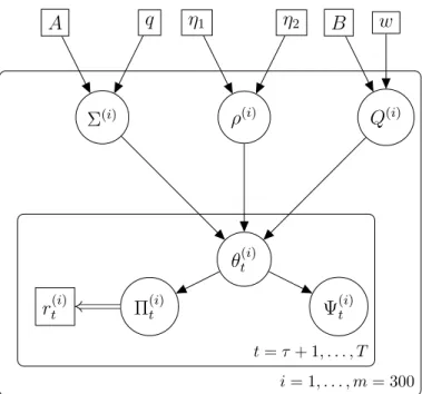
This thesis proposes three Bayesian estimation methods of the well-known Vector Error Cor-rection Model (VECM) about dierence stationary time series in order to extract the long-run equilibrium relationships. Each method used in this thesis is implemented using Markov Chain Monte Carlo (MCMC) and illustrated on synthetic data, and then on real economic data sets. The rst method consists of a static model, where we compare comovements between Eurozone economic time series comprising net trading, long-term interest rates and the harmonised unem-ployment rate. Primiceri (2005) established a time-varying model for the vector autoregressive model. Following Primiceri and the idea of the static model seen in the rst method, we are constructing a time-varying model for our VECM, from which we extract information about the time-varying cointegration matrix, and more interestingly about its time-varying rank (i.e. the cointegration rank) and independent cointegration relationships. These two rst methods are based on the singular value decomposition of the cointegration matrix from the error correction model and the so-called irrelevance criterion, a exible thresholding approach to determine its rank. In these two methods, the joint estimation of the cointegration rank and the cointegration relationships is deducted from synthetic data sets before applying them to real data sets (Euro-pean economies and major stock market exchange indices). The last main chapter of this thesis
covers the use of a prior singular distribution on the long-run relationship matrix of the VECM given the cointegration rank. Based on the denition of the singular matrix normal distribution proposed by Gupta and Nagar (2000), we also learn about the space denition and the density of such a distribution based on the work of Uhlig (1994) and Díaz-García et al. (2006). Gupta and Nagar (2000), Díaz-García et al. (1997) and Díaz-García and Gutiérrez-Jáimez (1997) also dene the singular Inverse-Wishart distribution and in our discussion, we eventually open the issues arising in implementing a dynamic model, by developing the idea of a singular Inverse-Wishart distribution on the variance covariance matrix of the transition equation (see Chapter 6).
Contents
1 Introduction 11
1.1 Background . . . 11
1.2 Aim of the thesis and layout . . . 13
2 Literature Review 16 2.1 Introduction to cointegration . . . 16
2.2 Denitions of cointegration . . . 18
2.2.1 Theory of cointegration . . . 19
2.2.2 The Dickey-Fuller test: Testing stationarity of time series . . . 20
2.3 Cointegration and Vector Error Correction Model . . . 26
2.3.1 Introduction to the Vector Error Correction Model . . . 26
2.3.2 Method to stack the data of the VECM in this thesis . . . 28
2.3.3 Johansen tests: Frequentist estimation of the cointegration rank . . . 30
2.3.4 Cointegrating relations and common trends . . . 30
2.4 Bayesian work on cointegration . . . 31
2.4.1 The Gibbs Sampler . . . 32
2.4.2 A prior on the cointegrating space . . . 33
2.4.3 A Bayesian estimation of the Error Correction Model including the coin-tegration rank: Villani (2005) . . . 34
2.4.5 Bayesian estimation of the lag order of the model . . . 39
2.4.6 Time-varying Bayesian estimation of the VECM . . . 39
2.4.7 Bayesian cointegration on other models than the VECM . . . 39
2.5 Estimation from a pre-sample . . . 40
3 Estimation of the cointegration rank and the coecients in a static model 43 3.1 Introduction . . . 43
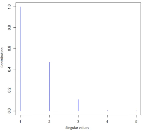
3.2 Approximation of the rank of Π . . . 45
3.3 Bayesian inference . . . 46
3.3.1 The likelihood of the VECM . . . 46
3.3.2 The prior distributions . . . 48
3.3.3 A prior of the rank implied by the prior of the singular values of the cointegrating matrix . . . 52
3.3.4 The posterior distributions . . . 53
3.3.5 The posterior distributions of Π and Ψunconditional on the variance ma-trixΣ . . . 54
3.3.6 Pre-sample and hyperparameters choice . . . 60
3.3.7 Obtaining the linearly independent cointegrating relationships from the matrix Π. . . 62
3.3.8 General Gibbs for a static Error Correction Model using a non-singular posterior distribution for Π and Ψ conditional on Σ . . . 63
3.4 Application . . . 65
3.4.1 Synthetic data sets and implementation . . . 65
3.4.2 The economic data sets . . . 70
3.4.3 Comparison with Johansen tests for the European panel data sets . . . 71
3.4.4 Comparison of the independent cointegrating relations with Villani . . . . 78
3.4.5 Interpretation of cointegrating relations . . . 79
3.4.7 Posterior summaries on the real data sets . . . 86
3.5 Discussion . . . 90
4 Time-varying cointegration 93 4.1 Time-varying Vector Error Correction Model . . . 93
4.2 State space models and estimating the parameters . . . 96
4.2.1 The general state space model . . . 96
4.2.2 State space model of the Vector Error Correction Model . . . 97
4.2.3 Forward Filtering and Backward Recursion of the Vector Error Correction Model . . . 99
4.2.4 Bayesian inference on the covariance matrixΣ . . . 100
4.3 Bayesian inference on the parameters of the transition equation: Q and ρ . . . 101
4.3.1 The likelihood of the transition equation . . . 101
4.3.2 Bayesian inference onρ: a uniform prior . . . 102
4.3.3 Bayesian inference onQ . . . 103
4.4 Initialization of the parameters and hyperparameters . . . 104
4.5 Time-varying cointegration: the rank and the cointegrating relations . . . 106
4.5.1 Evolution of the cointegration rank . . . 106
4.5.2 Evolution of the independent cointegrating relations . . . 106
4.6 Recapitulation of the algorithm . . . 107
4.7 Simulated data . . . 111
4.7.1 Description of the data . . . 111
4.7.2 Implementation of the code for the simulated data sets . . . 114
4.7.3 Estimation of the cointegrating parameters . . . 115
4.7.4 Posterior summaries . . . 123
4.8 Application to real data sets . . . 126
4.8.2 An application to the stock prices of three company sectors from the Dow
Jones Industrial Indices . . . 131
4.9 Discussion . . . 141
5 Cointegration analysis based on singular distributions 143 5.1 Introduction . . . 143
5.2 The matrix-variate normal singular distribution . . . 145
5.2.1 Denition . . . 145
5.2.2 A probability density function for the matrix-variate normal singular dis-tribution . . . 146
5.2.3 Method to simulate a matrix-variate normal singular distribution . . . 147
5.3 Prior distributions and the likelihood of the model . . . 149
5.3.1 Prior onΠ given S and Σ . . . 149
5.3.2 Issues in xingS . . . 150
5.3.3 Inference onS and introduction to a Bayesian hierarchical model . . . 151
5.3.4 Prior onΨ given Σ . . . 152
5.3.5 Prior onΣ . . . 153
5.3.6 The joint prior distribution and the likelihood . . . 153
5.4 Full conditional posterior distribution of the non-singular lag parameters: Ψ . . . 154
5.5 Bayesian inference on the non-singular variance matrix of the errors Σ. . . 157
5.6 Bayesian inference on the singular parameter of the VECM: Π . . . 159
5.6.1 Full conditional posterior distribution ofΠ . . . 159
5.6.2 Fixed cointegration rank . . . 167
5.7 Metropolis-Hastings to estimate the conditional distribution of U . . . 168
5.8 Gibbs sampler . . . 170
5.8.1 Setting of the hyperparameters . . . 170
5.8.2 Algorithm of the Gibbs sampler . . . 171
5.9.1 Application to the synthetic data set of Chapter 3 . . . 175
5.9.2 Sensitivity analysis around B . . . 175
5.9.3 Adjusting the acceptance rate of the Metropolis step with the variance C of the proposal distribution . . . 179
5.9.4 Posterior summaries . . . 184
5.9.5 Comparison with the static model of Chapter 3 for the European net tradings187 5.9.6 Application to six major stock market indices . . . 189
5.10 Discussion . . . 192
6 Consideration for future work: A dynamic VECM including a singular distri-bution for the time-varying cointegrating matrix 195 6.1 Introduction . . . 195
6.2 Bayesian inference about the transition equation . . . 196
6.3 Discussion . . . 198
7 Conclusions and future work 200 7.1 Conclusions . . . 200
7.1.1 Main ndings . . . 200
7.1.2 Advantages of the novel methods on Bayesian cointegration . . . 202
7.1.3 Limitations of these Bayesian estimations . . . 202
7.2 Future work and other directions . . . 203
APPENDICES 205 A Generalized inverse of a positive semi-denite matrix 205 A.1 Introduction and denition . . . 205
A.2 Solution of linearly-dependent equations . . . 206
A.3 The unicity of the generalized inverse of a positive semidenite matrix . . . 207 A.4 Decomposition of a positive semidenite matrix A with reduced diagonal matrix . 209
Notation
p∈N?, p≥2, 1≤ r < p. In this thesis, p denotes the number of time series used in a data set. T > p denotes the total length of the time series.
Mp,n(R) is the vector space of the real matrices of dimension p×n with n ∈N?.
Mp,p(R) is the vector space of the real square matrices of dimension p×p.
Dp(R)is the vector space of the real diagonal matrices of dimension p×p.
GLp(R)is the vector space of the real invertible matrices of dimension p×p.
S+
p (r) is the set of p×psemidenite positive matrices of rank r.
0p is the null element ofMp,p(R). Ip represents the identity matrix ofMp,p(R).
∀A ∈ Mp,n(R), A+ will dene the Moore-Penrose inverse of A. Op is the group of orthogonal p×pmatrices H, i.e. respecting HHT =HTH =Ip.
Vr,p is the set of matrices H ∈ Mp,r of full rank r and such that HTH = Ir. Vr,p is called the
Stiefel manifold.
Np×n(M, Q, P) with M ∈ Mp,n(R), P ∈ Mp,p(R) and Q ∈ Mn,n(R) represents the matrix
variate normal distribution seen in Chapter 2 of Gupta and Nagar (2000) with mean M and
covariance matrix P ⊗Q.
tp×n(M, P, Q, n) represents the matrix variate t-distribution seen in Chapter 4 of Gupta and
Nagar (2000) with location matrixM ∈ Mp,n(R), scale matricesP ∈ Mp,p(R)andQ∈ Mn,n(R)
and degrees of freedomn.
T N(η1, η2, µ, s)withη1 < η2denotes the truncated normal distribution with meanµand standard
Chapter 1
Introduction
1.1 Background
Economic time series are in general considered as trend dynamics or having a non-stationary behaviour over time. Such economic time series include stock market prices, foreign exchange rates, or macroeconomic variables, such as the unemployment rate, net trading and others. If a time series evolves as a random walk, then in the long run, the process will not be stable and the time series will grow or decrease without any limit. In this case it will become hard to predict the behaviour of these time series based on historical data, see Diebold and Kilian (2001). The principle of cointegration established by Granger (1981) allows the identication of economic time series that exhibit similar dynamics in the long run and the estimation of their relationships. This similarity is studied via the mean-reversion or stationarity of linear combinations of several time series.
Cointegration occurs for a set of integrated time series of order m if we can nd a linear
combination between them, that is integrated of lower order d < m, see Engle and Granger
(1987), Johansen (1996) and Johansen (1997). But in this thesis we will only consider dierence stationary time series (integrated of order 1), as it is often the case in econometrics, and we will propose methodologies to establish cointegration relationships between them that are stationary
(integrated of order 0). The cointegration rank, denoted generally asr in this thesis, represents
the number of independent linear combinations satisfying the property of stationarity. Our set of economic time series will then be said to be cointegrated of rank r, see Engle and Granger (1987).
After the groundbreaking work of Granger (1981) and Engle and Granger (1987), there has been a large literature on cointegration, see Johansen (1988), Johansen (1991), Johansen (1997), Phillips and Perron (1988) and Phillips (1991). Among Bayesian analysts, one can mention the works of Villani (2000), Strachan (2003), Kleibergen and van Dijk (1994) and Bauwens and Lubrano (1996). As for non-Bayesian analysts, Johansen (1997) developed two tests in order to evaluate the cointegration rank in a set of time series. These two tests are widely used for any study about cointegration.
A method that can come to mind in order to study the comovement between dierence stationary time series is to conduct an Ordinary Least Squares (OLS) regression. For instance let us consider an OLS regression between 2non-stationary time series xt and yt:
yt =βxt+ut
withutrepresenting the error terms andβ the slope of the regression. If our time series are
dier-ence stationary, then the error terms may be non-stationary and the regression would therefore incorrectly reject the null hypothesis H0 : β = 0. This comes from the fact that the estimatorβˆ
of the slope would not actually follow a Student distribution, leading to a spurious regression, see Banerjee et al. (1993), Damghani et al. (2012) and Granger and Newbold (1974). The regression results are then wrong, leading to a misinterpretation of the value of the coecientβ. However,
if we regress instead ∆yt with ∆xt by OLS: ∆yt = γ∆xt+vt with vt as a white-noise process,
then because ∆yt and ∆xt are stationary, the estimator ˆγ will be consistent.
By estimating the VECM, we actually take the lag dierence ∆xt of our VAR model xt and
determine the cointegrating matrix with a Bayesian approach (see Section 2.3). We will then avoid the case of spurious regression. One of the key points in the Bayesian approach is to choose a suitable prior distribution for the parameters of the VECM we want to estimate. We will see that the prior distribution implies the use of other parameters called hyperparameters, of which
one has to choose suitable estimates by appealing to certain methods (see for instance Section 3.3.2). Luetkepohl (2006) gives a method to estimate the parameters of the model that we will use to initialize the parameters in this thesis (see Section 2.5). The main parameter of interest in this thesis is the long-run relationships matrix obtained from the VECM. In this thesis, we focus on Bayesian inference of the cointegration matrix, by choosing a suitable prior and then derive a posterior distribution given the data and other parameters of the model. On the other hand, the likelihood can easily be derived from the distribution of the error terms in the VECM (see Section 3.3.1). Once both the likelihood and suitable priors are obtained, we can determine the full conditional posterior distributions of our parameters and run a Gibbs Sampler so that at the end we can get adequate estimates of the distribution of the parameters of the VECM.
1.2 Aim of the thesis and layout
This thesis introduces three methods to estimate the cointegration matrix: two methods are used to estimate static parameters (static methods) and the other method is about estimating time-varying parameters of the VECM (dynamic method). For the static methods as well as for the dynamic method, we will consider non-singular and singular Bayesian inferences around the cointegration matrix. In the non-singular Bayesian methods, we estimate the cointegration rank based on the singular values of the cointegration matrix (see Chapters 3 and 4). In the singular method, we dene a singular prior for the long-run impact matrix conditional on the rank (see Chapter 5).
First of all, a static model is used to compare the economies of the 4 biggest countries of the eurozone before and after the introduction of the single currency (see Chapter 3). This method starts from the VECM, from which priors are initialised on the parameters. In that model, we consider the long-run relationships matrix and the matrix of lag parameters as each having a non-singular multivariate normal prior distribution each, given the covariance matrix of the errors. This latter parameter will have an Inverse-Wishart prior distribution. Based on the likelihood of our model, we nd the three full conditional distributions wanted. But we decide to integrate
out the covariance matrix, in order to obtain matrix t-distributions for both the cointegrating matrix and the lag parameters matrix. This allows the Markov Chain Monte Carlo algorithm to run faster. For each cointegrating matrix simulated, an estimation of the rank is given by assessing the number of its most irrelevant singular values.
The second method consists of estimating a time-varying VECM (see Chapter 4), that we call the dynamic model, in order to dierentiate it from the static model, seen in the previous chapter. For that, a Forward Filtering Backward Recursion algorithm is employed. In that method we still dene a non-singular distribution for the cointegrating matrix. Since the cointegration matrix is time-varying, then the cointegration rank is also evolving over time. Then by using the same estimation of the rank on the time-varying cointegrating matrix as in the static method of Chapter 3, we are able to estimate a dynamic rank. Then from this dynamic rank and the dynamic cointegration matrix, we can easily obtain dynamic independent cointegrating relations. We can then obtain, for each time, an estimation of the rank and of the independent cointegrating relations. We test this novel method on a set of simulated data where we change on purpose the number of cointegrating relations over time. An application is then carried out on real data sets such as the European panel data seen in Chapter 3. We also decide to study the evolution of the cointegration rank in3sectors of the Dow Jones data set (see Chapter 4) from the year 2001
until 2009.
In Chapter 5, we go back to a static model but we establish a singular prior distribution on the long-run relationships matrix. Such a distribution may be called a reduced rank distribution. However, the prior singular distribution used on the cointegration matrix is based on knowledge of the rank. By xing the rank of the prior, we achieve the property of conjugacy and obtain a full conditional singular posterior distribution for the cointegrating matrix, with reduced rank the same as dened in the prior. The prior distribution of the cointegrating matrix is a singular normal matrix distribution, see Gupta and Nagar (2000) and Díaz-García et al. (2006). The lag parameter matrix still has a non-singular normal prior and the covariance matrix of the errors will have an Inverse-Wishart distribution. In this chapter, we will not integrate out the
variance of the errors and we will therefore have three full conditional distributions: the singular posterior distribution of the cointegrating matrix, the non-singular posterior distribution of the lag parameter matrix and the non-singular posterior of the covariance matrix of the errors. Unlike the 2 previous methods, we cannot estimate the rank in the MCMC procedure. We use
Johansen tests, see Johansen (1988), to assess the rank of the data, before running the algorithm. The property of conjugacy is veried and the MCMC algorithm uses a full conditional posterior singular distribution on the long-run impact matrix. The methods are applied on simulated data sets with a comparison with Chapter 3 and some real economic and nancial data sets.
Chapter 2
Literature Review
2.1 Introduction to cointegration
In general, most nancial time series are dierence stationary. Over many decades econo-metricians have been interested in developing models to study economic time series behaviours, see Keynes (1936). If we think about mathematical models such as autoregressive models, a white-noise process is used to represent the error terms in such models. This section introduces the advantages in choosing a Gaussian distribution for the error terms. In general, analysis of market data has shown that we can model economic time series as random walks, evolving as dierence stationary or unit root processes. The future of such time series cannot be predicted. This theory goes with the ecient-market hypothesis studied by Fama (1970):
xt =xt−1+ut ,ut ∼N(0, σ2)
whereutis a sequence of i.i.d. random variables following a normal distribution with mean0and
varianceσ2. With this hypothesis in mind, we can state that nancial markets are
information-ally ecient and therefore, we cannot predict returns given the information available at the time of investment. But there also exist many other types of dierence stationary time series. For example, the GDP of a country or its interest rate is not stationary, as it is typically exhibiting a trend.
However, in this thesis we believe in mathematical models in order to retrieve the facts that have occured in reality whether it is about the comovements in the Eurozone before and after the Euro (see Chapters 3 and 4) or in stock market indices (see Chapters 4 and 5). Financial data cannot be accurately predicted or evaluated only from geopolitical situations and intuition. Mathematical models are one of the most rational ways of predicting markets and often involves the knowledge of the trend in the past, or in a pre-sample before predicting more or less the behaviour of stock trends afterwards (e.g. comparing a moving-average time series and the real time series). For that reason and throughout many decades, investors have chosen to employ statisticians in order to make a decision on which stocks they should invest. Knowing events in the world and reading newspapers about nance are more than necessary in order to invest well, but it is not enough to understand comovements between such or such stocks. We can also bring that same argument to governments and their economies in the world.
The models proposed in this thesis are used to give an idea of which stocks or macroeconomic variables are potentially coevolving. Cointegration occurs when there exists a linear combina-tion of these non-stacombina-tionary time series, that is stacombina-tionary. Cointegrating relacombina-tions and their cointegrating coecients can inform us about the coevolution between these trend time series, see Johansen (2005), and inform a lot on market investment strategies. One of the recurring methods in which cointegration occurs is the pair trading strategy, see Schmidt (2008) and Rad et al. (2016). For instance, let us consider a pair of 2 stocks (Coca Cola and Pepsi) that are
cointegrated over a training sample. Suppose now that at this present date, the Pepsi index goes down compared to the Coca-Cola index. We therefore think that since both of these stocks are cointegrated, there is a high chance that the Pepsi index will go back up again, in order to catch up with the Coca Cola index and to satisfy the long-run cointegrating relationship. In that case, the investor might want to short sell a certain amount of stocks from Coca-Cola (when the value of Pepsi suddenly goes downwards), in order to buy at the same time for the same price a certain amount of stocks from Pepsi. At the time when Pepsi goes back up again, the investor can then sell the stocks from Pepsi and pocket a prot.
Cointegration in other areas than economics and nance
Cointegration is often used in econometrics or nance due to the frequency of integrated time series we encounter in these two elds. However, it is interesting to know that numerous works about cointegration have been applied to other elds such as, for instance, biology, socio-economic and environmental science panel data. Many elds can contain integrated time series and therefore cointegration techniques come naturally to assess relations between variables.
For instance, Chintrakarn and Herzer (2012) used panel cointegration techniques to investi-gate the eect of income inequality on crime in the United States. Kaufmann and Stern (2002) used cointegration to study co-movements between hemispheric temperature and the radiative forcing: solar irradiance, greenhouse gases, and tropospheric sulfates. Ostergaard et al. (2017) applied cointegration to a system of linearly phase coupled oscillating processes.
2.2 Denitions of cointegration
In this section, we recall general denitions on weakly stationary time series and the order of integration for a given time series. Any time series (xt)1≤t≤T of length T will be denoted as xt
in this section. We also assume that any time series has a known initial value x0.
Denition 1. Stationary time series
Let xt be a real time series. xt is said to be weakly stationary, if: ∀ t∈[[1, T]],
∃µ∈R , such that E[xt] =µ
∃σ ∈R , such that V ar[xt] =σ2
∀ h∈Z, ∃γh ∈R , such that Cov[xt+h, xt] =γh
Denition 2. Order of integration 0: Stationary
Let xt be a real time series. xt is said to be integrated of order 0 , denoted xt ∼ I(0) , or
trend stationary if xt is stationary.
Let xt be a real time series. xt is said to be integrated of order 1 , denoted xt ∼ I(1) , or
dierence stationary if ∆xt=xt−xt−1 is stationary, i.e., xt∼I(1) i ∆xt∼I(0).
Remark 1. xt ∼I(0)⇒xt∼I(1) is true but xt∼I(1)⇒xt∼I(0) is wrong!
A vector ut of time series integrated of order 1 is a vector for which each component is
integrated of order 1. It is denoted as ut ∼ I(1). We will use mostly the vector xt to describe
our time series xi,t.
2.2.1 Theory of cointegration
In this section, we consider a set of p dierence time series represented as a vector xt =
(xit)1≤i≤p, in which each componentxit represents the ith time series of our group at time t.
Denition 4. Cointegration
Ap-vector of dierence stationary time series xt(xt ∼I(1)) is said to be cointegrated
if there exists at least one non-zerop-vectorβ such thatβ0xt is trend stationary (i.e. β0xt∼I(0)). β is called a cointegrating vector.
Denition 5. Cointegration rank
If there exists r ∈ [[1, p−1]] linearly independent vectors βi, i ∈ [[1, r]] , such that βi
0
xt is
stationary, then xt is said to have cointegration rank r.
The r linearly independent p-vectors βi are called independent cointegrating relations.
They are stacked in a cointegration matrix denoted as β = (β1, β2, ..., βr) in this thesis.
Granger (1981) and Engle and Granger (1987) were the rst to develop the notion of cointe-gration. Later on, Johansen (1988, 1991, 1996, 1997, 2005, 2006) will introduce several statistical tests to determine the cointegration rank. In addition, the cointegration rank can be thought as an index of how well time series are co-evolving: the bigger the cointegration rank is in a set of time series, the more comovements will be present in that set of time series.
2.2.2 The Dickey-Fuller test: Testing stationarity of time series
Establishing cointegrating relationships requires the need to test if the linear combination of our time series, i.e. the cointegrating relation, is stationary. For that matter, several statistical tests are employed in order to evaluate if a time series is stationary or not: Phillips and Perron (1988), Kwiatkowski et al. (1992) (KPSS) and Dickey and Fuller (1979). We focus in this chapter on the Dickey Fuller test.
Let us rst consider a simple autoregressive model AR(1) represented by:
xt=φxt−1 +et , ∀t ∈[[1, T]]
where φ and x0 are real numbers and where et iid
∼ N(0, σ2) with σ2 >0.
Let us now study the following three dierent cases leading to the conclusion ifxtis stationary
or not:
1. |φ|<1⇒xt is stationary:
Since |φ|<1, then one has:
xt =φxt−1+et ⇐⇒ xt−φxt−1 =et ⇐⇒ (1−φB)xt=et
with B being the backward shift operator. If|φ|<1 then (1−φB) is invertible and:
(1−φB)−1 =
∞
X
i=0
φiBi
Then we can write:
xt= (1−φB)−1et= ∞ X i=0 φiBiet = ∞ X i=0 φiet−i
Since all theet are independent we have ∀t ∈N∗,
(a) E[xt] = P∞ i=0φ iE[e t−i] = 0 , (b) V ar[xt] =P ∞ i=0φ 2iV ar[e t−i] =P ∞ i=0φ 2iσ2 =σ2P∞ i=0φ 2iand thenV ar[x t] =σ21−1φ2 = σ2 1−φ2.
(c) ∀h∈ {1, ..., T −t}, Cov[xt+h, xt] =Cov[ ∞ X j=0 φjet+h−j, ∞ X i=0 φiet−i] = ∞ X i=0 ∞ X j=0 φi+jCov[et+h−j, et−i]
Then, since Cov[et−i, et+h−j]6= 0 ⇐⇒ t−i=t+h−j ⇐⇒ j =h+i, then we have
∀ t, Cov[xt+h, xt] = ∞ X i=0 φ2i+hσ2 =φhσ2 ∞ X i=0 φ2i = φ hσ2 1−φ2
proving thereby stationarity. 2. |φ|= 1⇒xt is not stationary.
If|φ|= 1, then φ=±1and then we can write:
xt = t−1 X i=0 φiet−i+φtx0 Then we have: ∀t >0, E[xt] = t−1 X i=0 φiE[et−i] +φtx0 =φtx0
and we can see that the expectation of xt is not constant if and only if x0 6= 0, and then
the vector of time series xt is not stationary.
Ifx0 = 0, then the expectation is constant and equal to0. But in that case if we write the
variance ofxt, we get: V ar[xt] =V ar[ t−1 X i=0 φiet−i+φtx0] = t−1 X i=0 φ2iV ar[et−i] =σ2 t−1 X i=0 1 = σ2t
and we can clearly see that the variance of xt is not constant and thus the time series is
not stationary.
3. |φ|>1⇒xt is not stationary.
In that case we can use similar computations to write the variance ofxt as:
V ar[xt] = t−1 X i=0 φ2iV ar[et−i] =σ2 t−1 X i=0 φ2i
Since|φ|>1, thenφ2 >1and therefore the above time series diverges asttends to innity.
Therefore we conclude thatxt is non-stationary.
The Dickey-Fuller distribution
Dickey and Fuller (1979) developed a test for detecting the presence of a unit root in an autoregressive model. If a unit root is present then it means that the process is not stationary. This test uses critical values corresponding to a distribution called the Dickey-Fuller distribution which depends also on the sample size.
Let us take the example of a process without deterministic terms based on T observations x1, x2,..., xT:
xt=φxt−1 +et , ∀t ∈[[1, T]]
where et iid
∼N(0, σ2).
Given these T observations x1, x2, ..., xT, the maximum likelihood estimator of φ is obtained
from the moment condition, i.e. that the error termset and the time seriesxt are uncorrelated:
E[etxt−1] = 0 =⇒ T X t=1 etxt−1 = T X t=1 (xt−φxˆ t−1)xt−1 = 0 Hence: ˆ φ= PT t=1xtxt−1 PT t=1x2t−1
The Dicky-Fuller test is based on the following statistic:
ˆ
f = φˆ−1
SE( ˆφ)
where SE( ˆφ)is the usual standard error estimate. Then we can write fˆas:
ˆ f = ˆ φ−1 S/( q PT t=2x2t−1) = PT t=2(∆xt)xt−1 S q PT t=2x2t−1
where S is the unbiased estimator of σ2: S2 = T1−2PT
t=2(xt−φxtˆ −1)
2. Using the fact that S2 is
consistent, that is, S2 converges in probability to σ2 (asT takes large values), we obtain:
ˆ f = 1 T PT t=2(∆xt)xt−1 S q 1 T2 PT t=2x2t−1 (2.1)
Phillips and Perron (1988) proved that the sample moments of {xt} converge to functions of
Wiener processes: A=T−1 T X t=1 xt−1t d →σ2 Z 1 0 W(r)dW(r) B =T−2 T X t=1 x2t−1 d →σ2 Z 1 0 W(r)2dr where d
→means "converges in distribution to. Now, as T tends to innity we have:
ˆ f = A S√B d −→X = R1 0 W(r)dW(r) q R1 0 W(t) 2 dt (2.2)
where {W(t), t ≥0} is the standard Wiener process, see Phillips and Perron (1988).
The asymptotic distribution of the Dickey-Fuller statisticfˆ(2.1) is in fact a functional of the
Wiener process. This asymptotic distribution of fˆis called the Dickey-Fuller (DF) distribution
and does not have any closed form representation. The quantiles and critical values are therefore derived from numerical approximations or simulations (see Figure 2.1).
In order to approximate the Dickey-Fuller distribution, we will need to simulate several times a random walk of a given time length T:
xt=xt−1+et , ∀t∈[[1, T]]
with et iid
∼N(0, σ2).
If we simulate N random walks, then we can extract N values fˆ(2.1), that will build our
Dickey-Fuller distribution (see Figure 2.1). The approximation is more accurate when the number
N gets bigger, that is the number of random walks simulated. From theN dierent values of fˆ
Figure 2.1: Simulated Dickey-Fuller distribution
The histogram in Figure 2.1 is constructed based on 1,000 simulations of X from the
ex-pression derived in (2.2). Based on this histogram and with a lot of simulations of the random variable X, we are able to determine an approximation of the 10%,5% and 1% quantiles.
Instruction and explanation of the test
From a data set measured from t= 1 to t=T (with T >1), we can calculate the statistic fˆ
from Equation (2.1). The null hypothesis of the Dickey-Fuller test is:
H0 : ˆf ≥0 i.e. φˆ= 1, or xt is not stationary H1 : ˆf <0 i.e. φ <ˆ 1, or xt is stationary
From the simulated Dickey-Fuller distribution (see Figure 2.1), we obtain the quantiles -2.451, -1.992, -1.603, that is:
P(X <−1.992) = 0.05
P(X <−1.603) = 0.10
If for example fˆ=−1.7 we will reject the null hypothesis of non-stationarity (i.e. consider
the process xt to be stationary) at risk 10%. On the other hand we will not reject the fact
that it is not stationary at risk 5%. We can also directly look at the p-value of the test which
corresponds to the value of P(X ≤ fˆ). If that p-value is lower than 10% but greater than 5%
we will draw the same conclusion.
The Augmented Dickey-Fuller test
Said and Dickey (1984) augmented the basic autoregressive unit root test to time series of unknown lag orderk > 1. This test is called the Augmented Dickey-Fuller (ADF) test. The ADF
test tests the null hypothesis that a process xt is dierence stationary against the alternative
that xt is trend stationary. This ADF test is based on estimating the test regression:
xt=φxt−1+
k
X
j=1
ψj∆xt−j +γ0Dt+t
whereDtis a vector of deterministic terms (constant, trend, etc.). But again, as mentioned above
the deterministic part of the equation is not taken into account throughout this thesis. The k
terms ∆xt−j are called the lagged dierence terms. Under the null hypothesis, xt is dierence
stationary, i.e. ∆xt=xt−xt−1 is stationary, which impliesφ = 1.
In fact, an alternative formulation of the ADF test regression is:
∆xt=πxt−1+
k
X
j=1
ψj∆xt−j +γ0Dt+t
where π = φ−1. Under the null hypothesis, ∆xt is stationary which entails that π = 0. The
ADF test statistic is then the statistic for testingπ = 0:
ADFt= ˆ π SE(ˆπ) = PT t=2(∆xt)xt−1 S q PT t=2xt−12
with S2 = T−12PT
t=2(xt−
Pk
j=1∆xt−j)
2 which is an unbiased estimator of σ2 because:
E[S2] = Eh 1 T −2 T X t=2 (xt− k X j=1 ∆xt−j)2 i = 1 T −2 T X t=2 E[(xt− k X j=1 ∆xt−j)2] = 1 T −2 T X t=2 E[2] = 1 T −2(T −2)σ 2 =σ2
2.3 Cointegration and Vector Error Correction Model
2.3.1 Introduction to the Vector Error Correction Model
Most of the research papers about cointegration use the Vector Error Correction Model to retrieve the cointegrating relations (see Engle and Granger (1987) and Villani (2005)). This model indeed provides a cointegrating matrix, from which independent relationships are derived as well as the cointegration rank. If we consider (xt)tt==1T as a realization of the p-dimensional
Vector Autoregressive (VAR) process of lag length k ∈N?, then: xt =
k
X
i=1
Γixt−i+t (2.3)
with t∼Np(0p,Σ)and Σ a positive denite matrix (Σ>0).
From there, we can obtain the Vector Error Correction Model (VECM) by taking the lag dierence of order 1 ∆xt =xt−xt−1: ∆xt= Πxt−1+ k−1 X i=1 Ψi∆xt−i+t (2.4) with t∼Np(0p,Σ).
(2.4): Ψj =−(Γj+1−...−Γk) = − k X i=j+1 Γi, ∀j ∈[[1, k−1]] (2.5) Π =−(Ip−Γ1−Γ2−...−Γk) = −(Ip− k X j=1 Γj) (2.6)
From Equation (2.4), we can isolate the term Πxt−1 on one side of the equation: Πxt−1 = ∆xt−
k−1 X
i=1
Ψi∆xt−i−t (2.7)
Our vector of time series xt = (xit)1≤i≤p is composed of p integrated processes xit of order
1: xit ∼ I(1). Thus, each rst dierence lag vector of time series {∆xt−j}0≤j≤k−1 will be a
vector of stationary processes. Since the error processes vector t = (it)1≤i≤p is also composed
of stationary signalsit ∼I(0), then by operation, the right hand side of (2.7) is also stationary.
ThereforeΠxt−1 is equal to a vector of stationary processes:
Πxt−1 =vt= (vit)1≤i≤p with eachvit ∼I(0) (2.8)
The matrix Π, called the long-run impact matrix, is a cointegrating matrix from which each
row constitutes a cointegrating vector inRp. Then, depending on the rank ofΠ, we have3cases.
Case 1: The cointegrating matrix Π is of full rank
If the cointegrating matrix Π is of full rank, i.e. the rank of Π isp, then Π is invertible and,
from equation (2.8) above, we will have for eacht: xt−1 = Π−1vt. From this point we can deduce
by operation that each component xit of xt is a stationary time series.
In this particular case, Π is invertible and the rows of Π are p independent cointegrating
relations.
Case 2: The cointegrating matrix Π is of lower rank r∈[[1, p−1]]
In this case, the rank of Π is supposed to be not full and equal to 1 ≤ r < p. This rank is
rank decomposition theorem, see Banerjee and Roy (2014), we know that we can derive at most
r independent cointegrating relationships from Π. We can indeed decompose Π into a product
αβ0 where α and β are 2 matrices of Mp,r(R) of full rank r, see Puntanen et al. (2011).
We can obtain from (2.8) thatΠxt−1 =αβ0xt−1 =vt= (vit)1≤i≤p with eachvit∼I(0). Then,
by operation, we can obtain:
β0xt−1 =ut= (uit)1≤i≤r with eachuit ∼I(0) (2.9)
Therefore, therindependent cointegrating relations are obtained from therrows of the matrix β0, or the r columns of matrix β. Matrix β will therefore give the independent cointegrating
relations.
Case 3: The cointegrating matrix Π is of rank 0
If the rank of Π is 0, then Π is the null element ofMp,p(R), and there is no cointegration.
2.3.2 Method to stack the data of the VECM in this thesis
This section describes how we stack the data so that we can dene a general likelihood of the VECM, taking into account all the data we have from time 1to time T. We assume a lag order k ≥2 to be known for the VAR model from which the VECM is dened. We have:
∆xt = Πxt−1+
k−1 X
j=1
Ψj∆xt−j+t (2.10)
Firstly, we dene the p×p (k−1) matrix Ψ gathering the lag parameter matrices of the
VECM given by Equation (2.10):
Ψ = [Ψ1,Ψ2, . . . ,Ψk−1]
Then we dene for each timet∈[[1, T]], the vectorzt, of sizep(k−1), containing respectively
[∆xt−1, ∆xt−2, ... , ∆xt−k+1], i.e.
zt=
h
∆x0t−1 ∆x0t−2 · · · ∆x0t−k+1
We can now write (2.10) as :
∆xt= Πxt−1+ Ψzt+t (2.11)
Then, by denoting each ∆xt as yt, we can transpose both sides of the expression (2.11) and
obtain:
yt0 =xt−10Π0+zt0Ψ0+t0 (2.12)
Let us assume now that x−k, x−k+1, ..., x0 exist and are provided. Then we can create the
matrix Y of size T ×p, that gathers all theyts of Equation (2.12) from t= 1 tot=T:
Y =hy1 y2 · · · yTi
0
=h∆x1 ∆x2 · · · ∆xTi
0
We also create the matrix X of size T ×p, that gathers all xt−1 from t= 1 to t=T:
X =hx0 x1 · · · xT−1i
0
Then, we create the matrix Z of size T ×p(k−1), that gathers all zt fromt= 1 tot=T:
Z =hz1 z2 · · · zT
i0
Finally the matrix of the errors E of size T ×p, that gathers all the errors t from t = 1 to t=T, is:
E =h1 2 · · · Ti
0
(2.13) Therefore, the t-th row of X, Y, Z and E are respectively x0t−1, ∆x0t, [∆x0t−1, . . . ,∆x0t−k+1]
and 0t. In this thesis, we will often dene "the information brought by the data by the set
D={X, Y, Z}. We can write the total VECM system, based on the data from D, as:
Y0 = ΠX0+ ΨZ0+E0 (2.14)
Then, by transposing the above expression (2.14), we can also obtain:
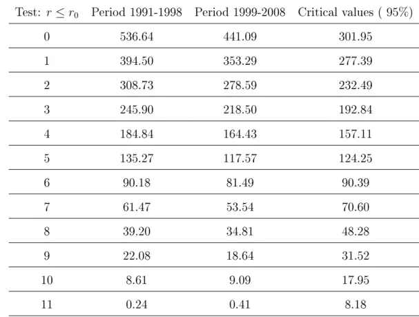
2.3.3 Johansen tests: Frequentist estimation of the cointegration rank
Johansen (1991) elaborated two types of tests for cointegration. These tests in fact study, for each cointegration rank r assumed, if the r independent linear combinations for a set of p time
series give stationary processes.
The two tests that Johansen elaborated are the Maximum Eigenvalue test and the Trace test. The Maximum Eigenvalue test examines the null hypothesis if the cointegration rank r is equal
to a certain value r0 against the alternate hypothesis that it is r0+ 1. The Trace test examines
the null hypothesis that the number of linear combinationsr is equal to a given valuer0 against
the alternative hypothesis that the cointegration rank r is greater than r0.
2.3.4 Cointegrating relations and common trends
If the matrix Π has rank r, then we can decompose Π into the product of two p×r full
rank matrices α and β as Π =αβ0. Then, since matrix β is of full rank, the columns of β will
representr independent cointegrating relations.
According to Johansen (1988) and Johansen (1991), we can nd ap×(p−r)matrixβ⊥, that
is orthogonal to β, i.e. β0β⊥ = 0, and such that the p×p matrix G = [β, β⊥] is invertible. The
matrix β⊥ is called the common trends loading matrix, see Johansen (1988), Johansen (1991)
and Stock and Watson (1996).
If we have for example a vector ofptime seriesxtof which we ndrindependent cointegrating
vectors stacked as the columns of β, then the space spanned by β0xt is called the cointegrated
space of the set of time series xt and the space spanned by β⊥0xt is called the unit root space of xt. The number of common trends is in fact equivalent to the number of time series subtracted
to the number of independent cointegrating relations. Stock and Watson (1996) proposed tests to evaluate the number of common trends rather than the number of cointegrating relations. Their tests are applied to U.S. postwar interest rates.
2.4 Bayesian work on cointegration
Since the work of Sims (1988), who advocated the Bayesian paradigm for unit root testing, there has been a growing interest in Bayesian cointegration as evidenced by Schotman and van Dijk (1991), Kleibergen and van Dijk (1994), Strachan (2003), Bauwens and Lubrano (1996), Vil-lani (2005), Conigliani and Tancredi (2009) and Meligkotsidou et al. (2014). A good review of the Bayesian approach to cointegration is given in Koop and Tobias (2006). Considering multivariate unit root testing, there appears to be two main points of interest (a) estimating the number of cointegrating relationships (i.e. the cointegration rank) and (b) estimating the coecients which take part in these cointegrating relationships, usually adopting the vector error correction model (VECM) introduced by Engle and Granger (1987). For example, Villani (2005) estimates the parameters of the error correction model conditional on the cointegration rank, by splitting the cointegrating matrix Π into two full rank matrices α (matrix of adjustment coecients) and β
(matrix containing the independent cointegrating vectors). Given the cointegration rank, Villani then derives a full conditional posterior distribution for the parameters α, β, Ψand Σ. Besides,
Villani (2005) derives a posterior distribution conditional on the data for the cointegration rank. A Bayesian analysis of cointegration is very useful because it produces a distribution rather than a point estimate of the parameters used to establish cointegration. We can obtain more information (credible intervals, mode, median, mean) than a simple estimate. Multivariate coin-tegration methods oer an important framework of identifying relationships between nancial time series, hence are often exploited in developing long term decision making, trading and port-folio management. We propose in this thesis a Bayesian analysis of the Error Correction Model, using Markov Chain Monte Carlo methods (MCMC) in a static or dynamic context.
As part of the literature on Bayesian cointegration, Koop et al. (2006) provides a detailed summary of Bayesian methods developed in the last thirty years. We will recapitulate them in some of the next sections in this chapter (see Sections 2.4.2, 2.4.3, 2.4.4).
2.4.1 The Gibbs Sampler
The Gibbs sampler is a Markov Chain Monte Carlo algorithm (or MCMC), that allows us to obtain a sequence of observations that are approximately sampled from a specied multi-variate probability distribution. This sequence is then used to approximate the joint posterior distribution of the parameters of a model. The idea of sampling comes from the physicist and researcher J. W. Gibbs who wanted to make an analogy between the sampling algorithm and statistical physics. The work of Casella and George (1992) gives more details about the idea of Gibbs sampling. Although the principles of the Gibbs algorithm were to be used in physics, they are also widely used in econometrics, and are also applicable to the mathematical models of many elds (biology, weather forecasting, etc.). Let us assume we have a model where we want to determine parameters θj, j ∈[[1, h]]. We decide to represent the set of parameters in a vector
of parameters θ:
θ =θ1 θ2 · · · θh
0
The Gibbs sampler begins with an initial vector of parameters, calledθ(0). Those initial values
will be assumed to be known at the beginning in order to explain the Gibbs sampling algorithm. Initial values can usually be determined from a pre-sample, but also given subjectively. We will recall later some methods developed in the thesis in order to have suitable initial conditions for the Vector Error Correction Model. The ith draw of a parameter in the Gibbs sampler will be
denoted by θ(i). The ith draw of θ is obtained by collecting sequentially and in the right order
the h draws from the full conditional posteriors for θj , withj = 1, ..., h, where:
θ(ji)∼p(θj|θ (i) 1 , ..., θ (i) j−1, θ (i−1) j+1 , ..., θ (i−1) h ,D)
where j = 1, ..., h and i= 1, ..., g. In the end we collect the ith drawn vector
θ(i)=θ(i) 1 θ (i) 2 · · · θ (i) h 0
θ(i) is a draw from the joint posterior distribution p(θ|D), where D represents the data or
simulated at each stepi from:
θ(i) = (θ1(i),· · · , θj(i−)1, θj(i), θj(i+1−1),· · · , θh(i−1))∼p(θ|D)
Hence, θ(i) is also a draw from the joint posterior distribution ofθ. Bauwens and Giot (1998)
use a Gibbs sampling approach to cointegration by applying it to a cointegrated Vector Au-toregressive system and therefore derive the cointegrating relations from a Bayesian perspective. Similarly, Villani (2005) makes use of the Gibbs sampling method to estimate the parameters of the Error Correction Model.
2.4.2 A prior on the cointegrating space
It may also be of interest to mention from the literature some Bayesian works around the possibility of setting a prior on the cointegrating space, i.e. the space spanned by the independent cointegrating vectors: sp(β). Villani (2005) and Strachan and Inder (2004) adopted this novel
approach where sp(β)becomes the centre of interest rather than the values of the cointegrating
coecients β.
The cointegrating space sp(β) is generally denoted as þ in the literature. For Strachan and
Inder (2004) þ=sp(β)is actually a random parameter taking values in the Grassmann manifold
Gr,p−r. We recall thatVr,p is the set of matricesH ∈ Mp,r of full rankrand such thatHTH =Ir
(orthogonal matrices). If the p×r matrix β ∈ Vr,p, then the space spanned by the matrix β is
in the Grassmann manifoldGr,p−r: þ=sp(β)∈Gr,p−r.
Villani (2005) and Strachan and Inder (2004) use a uniform prior on þ, which can be obtained from a prior distribution ofβ onVr,p. A draw from a uniform prior overVr,p can be obtained by
the operation β =Z(Z0Z)−1/2 where V ec(Z)∼N(0, Ipr). Then the space spanned by β will be
uniformly distributed overGr,p−r. Villani (2005) in Lemma 3.4 states that if we haveβ = (Ir B0)0
withB ∼t(p−r)×r(0, Ip−r, Ir,1), thenβ will be uniformly distributed over the Grassman manifold Gr,p−r. Villani then derives a matrix variate normal full conditional posterior distribution forB,
see Theorem 4.5, Villani (2005).
prior on the cointegrating space. We will assume that we havep= 3economic time seriesx1t,x2t
andx3twith cointegration rankr= 2. If we have an idea of what the2independent cointegrating
coecients are (for instance,x1t−β1x2t∼I(0) and x2t−β2x3t ∼I(0)), then we can dene the
matrix H as: H = 1 0 −β1 1 0 −β2 We have that þh
=sp(H)is a value in Gr,p−r. Strachan and Inder (2004) propose a prior for
the random parameter þ where its mass is centered around þh. For that, they dene the p×p
random matrixPτ as:
Pτ =HH0+H⊥H⊥0τ
where τ is chosen as being a scalar random variable normally distributed asτ ∼N(0, στ2).
Then, by dening a random p×r matrix Z distributed as V ec(Z)∼N(0, Ipr), we construct
the matrix X = PτZ that can be decomposed later on as X = βκ, where κ is an r×r lower
triangular matrix. The dispersion around þh is controlled by the chosen value of the variance of τ, i.e. στ2.
2.4.3 A Bayesian estimation of the Error Correction Model including
the cointegration rank: Villani (2005)
A very interesting paper on Bayesian estimation of the Vector Error Correction Model was developed by Villani (2005). Conditional on the cointegration rank r, Villani (2005) splits the
cointegrating matrix Π into 2 full rankp×r matrices α and β and infers these two latter.
In Villani (2005), the VECM is then constructed as the following, conditional on the cointe-gration rank r: ∆xt =αβ0xt−1+ k−1 X i=1 Ψi∆xt−i+t (2.16)
with t∼Np(0p,Σ).
Villani (2005) then infers α, β, Ψ and Σ conditional on r by building rst the joint prior
distribution of these four parameters. The prior of Σ is an Inverse-Wishart: Σ ∼ IW(A, q)
where A >0and q are two hyperparameters. A uniform prior is dened on Ψ = [Ψ1,· · · ,Ψk−1]
and the prior of α is Gaussian and conditional on β and Σ: α ∼Np×r(0,(β0β)−1, v−1Σ) with v
as a hyperparameter. As forβ, Villani (2005) sets a uniform prior on the cointegration space by
using the form β = (Ir B0)0 with B ∼t(p−r)×r(0, Ip−r, Ir,1). Finally the joint distribution of α ,
β,Ψ and Σ conditional on r is given by: f(α, β,Ψ,Σ|r)∝cr|Σ|− p+r+q+1 2 exp −1 2Tr(Σ −1(A+vαβ0βα0)) (2.17) where cr is a scalar depending on r.
The likelihood is constructed on the error terms of the VECM (2.16), each having a normal distribution with covariance matrixΣ: t∼N(0,Σ). Hence,
f(D|α, β,Ψ,Σ, r)∝f(V ec(E0)|α, β,Ψ,Σ, r)∝ |Σ|−T2 exp −1 2Tr(Σ −1E0 E) (2.18) where E0 =Y0 −ΠX0−ΨZ0 from equation (2.14) will contain α, β (by Π =αβ0) and Ψ.
As for the cointegration rank, the prior distribution f(r) is a discrete uniform distribution
over the space [[0, p]], i.e. f(r = ν) = 1
p+1 for each ν ∈ [[0, p]]. Villani (2005) then derives the
posterior distribution of the cointegration rank that is conditional on the data D only:
f(r|D) = Ppf(D|r)f(r)
r=0f(D|r)f(r)
(2.19) Villani (2005) obtains this posterior distribution of the cointegration rank by integrating out
Σ, Ψ, α and β, in order to obtain the marginal likelihood of the data given the cointegration
rankf(D|r):
f(D|r) =
Z Z Z Z
f(D|α, β,Ψ,Σ, r)f(α, β,Ψ,Σ|r) dΣdΨ dα dβ (2.20)
The cointegration rank r will therefore have a posterior distribution conditional on the data
distribution of r will have more mass around certain values. Villani (2005) uses a bivariate
process in order to assess the probability of three dierent values for the rank: f(r = 0|D),
f(r = 1|D) and f(r = 2|D). The other parameters of the VECM such as α and β are also
estimated. Following the methods of Villani (2005), an application to the demand for the Euro Area was performed by Warne (2006).
2.4.4 The embedding approach on the Error Correction Model
Let us consider an Error Correction Model as in (2.16) in which the rank is established to be
r < pand the matrix Π is split into 2 full rank p×r matrices α and β. For this section, we will
call that model the Error Correction Cointegration model (ECC model).
The embedding approach involves the existence of a parameter matrix that will evaluate the degree of the rank of Π. Let us now construct a model called the Unrestricted Error Correction
model (UEC model) by adding a (p−r)× (p− r) parameter matrix λ making the long-run
relations matrix Π to be of full rank. We can write the long-run relations matrix Π as:
Π =αβ0 + 0 Ip−r λ h 0 Ip−r i (2.21) where α=hα10 α20 i0 and β0 =hIr B0 i
We have α1 of size r×r, α2 of size (p−r)×r and B
of size (p−r)×r.
If we now write Π as:
Π = Π11 Π12 Π21 Π22 (2.22)
where Π11 is of size r×r, Π12 is of size r×(p−r), Π21 is of size (p−r)×r and Π22 is of size (p−r)×(p−r), then thanks to (2.22), we can identify the expressions of α, B and λ from
We have:
α1 = Π11 (2.23)
α2 = Π21
B0 = Π11−1Π12
λ = Π22−Π21Π11−1Π12
However, a problem of local non-identication can occur when Π11 is not invertible, in which
case λ and B are diverging. An embedding model will be constructed in order to nest various
Error Correction Cointegration models according to dierent values of r. The embedding model
approach was rst investigated by Kleibergen and van Dijk (1994) and then by Kleibergen and Paap (2002).
Kleibergen and Paap (2002) proposed a singular value decomposition ofΠ in the UEC model
as: Π =U SV0 = U11 U12 U21 U22 S1 0 0 S2 V110 V210 V120 V220 (2.24)
where by denitionU andV are orthonormal matrices andS is a diagonal matrix containing the
singular values of Π (of the UEC model) in descending order. This implies thatS2 is a diagonal
matrix containing thep−r smallest singular values of Π.
By using (2.24) and (2.21), we can retrieve the parameters:
α0 =V11S1[U110, U210] B =V11−1V12 λ= (V220V22)− 1 2V22S2U220(U220U22)− 1 2
In that way, there is no local non-identication issue since V220V22 and U220U22 are both
invertible (unitary matrices). Kleibergen and Paap (2002) then use the help of Bayes factors in order to assess a posterior probability distribution for the cointegration rankr. At rst, they set
construct a prior odds ratio function consisting of the ratio between the prior probability of rank
r and the prior probability of full rank r =p:
P ROR[r|p] = P[rank=r]
P[rank=p] (2.25)
A Bayes Factor BF[r|p] for each rank r is then constructed as follows:
BF[r|p] = P[D|rank=r]
P[D|rank=p] (2.26)
P[D|rank=r] is computed by integrating out Σ, Ψ, α and β from the joint posterior of the
parameters of the ECC modelfECC(α, β,Ψ,Σ|D)(conditional on the rank):
P[D|rank=r] =
Z Z Z Z
fECC(α, β,Ψ,Σ|D) dΣdΨ dα dβ
P[D|rank = p] is computed by integrating out Σ, Ψ, α, β and λ from the posterior of the
parameters of the UEC model fU EC(λ, α, β,ΨΣ|D):
P[D|rank=p] = Z
· · · Z
fU EC(λ, α, β,Ψ,Σ|D) dΣdΨdα dβ dλ
If the Bayes Factor (2.26) is larger than 1, then the model of rank r is preferred to the full
rank model. Thanks to Equations (2.25) and (2.26), we can obtain the posterior odds ratio (2.27) below:
P OR[r|p] =P ROR[r|p]×BF[r|p] (2.27)
Then, from all the posterior odds ratios P OR[r|p] derived for each r ∈[[0, p]], we can obtain
a posterior distribution for the rankr:
P[rank=r|D] = PpP OR[r|p]
r=0P OR[r|p]
(2.28) Kleibergen and Paap (2002) estimate the cointegration rank between real money supplyM2,
real income, price level and costs of holding money in Denmark by using the posterior distribution of the rank given the data, i.e. Equation (2.28). They nd a cointegration rank in favor of 1for
an Error Correction model considering a restricted constant by using the fact that the posterior probability P[rank= 1|D]is the highest. Besides, all restricted models are more likely than the
2.4.5 Bayesian estimation of the lag order of the model
As for the lag orderk, it can enter into the model as a parameter on which Bayesian inference
can be performed. Phillips (1996), Corander and Villani (2004) and Chao and Phillips (1999) estimate the posterior distribution for the lag order jointly with the cointegration rank.
2.4.6 Time-varying Bayesian estimation of the VECM
In the literature about time-varying Bayesian cointegration, it is worth mentioning a few works on the time-varying Error Correction Model (ECM). To start with, Granger and Lee (1991) introduced a time-varying cointegrated process that they applied to US data prices and wages. Bierens and Martins (2010) propose a time-varying ECM where the cointegrating rela-tions change smoothly over a certain time period. These works assume a constant cointegration rank and focus more on the values of the cointegrating coecients evolving over time.
Koop et al. (2011) also developed a dynamic ECM in which he considers the cointegrating space (see Section 2.4.2) evolving over time. He introduces a Markov Chain Monte Carlo pro-cedure and an algorithm for state space models in order to infer the time-varying ECM. Koop et al. (2011) showed the behaviour over time of one cointegrating relation between US economic variables.
2.4.7 Bayesian cointegration on other models than the VECM
A signicant amount of Bayesian works around cointegration do not involve the use of the Error Correction model , such as DeJong (1992), Dorfman (1994), Koop (1991) and Koop (1994). Let us consider a VAR model (2.3) for the p-dimensional process xt composed of
dierence-stationary elements such as xt = Pk
j=1Γjxt−j +t with t ∈ [[1, T]] and we can write the VAR
representation as: (Ip− k X j=1 ΓjLj)xt=t (2.29)
where Lj is the lag operator raised to the integer powerj.
The number of independent cointegrating relations is estimated from the number of non-stationary roots of the VAR model: the elements of xt will be cointegrated if (Ip−
Pk
j=1Γjzj)
has 0 < p−r < p non-stationary unit roots. In such a case, there exist r cointegrating vectors βi such thatβi0xt is stationary.
DeJong (1992) uses non-informative uniform priors on the Γj coecients in order to derive
posterior distributions from which draws are made thanks to Monte Carlo integration methods. We can obtain the roots of the VAR representation by constructing their posteriors based on the simulatedΓj coecients. By still using the approach of the number of non-stationary roots in a
VAR model, Dorfman (1994) develops a Bayesian cointegration test focusing on the posterior odds of the number of unit roots in the set of integrated processes. DeJong (1992) and Koop (1991) use this approach to verify common behaviours between stock prices and dividends. Koop (1994) also detects common trends between spot and forward exchange rates from dierent countries (USA, Canada, Germany and the UK). Apart from between stocks and dividends, DeJong (1992) investigates these methods of nding cointegration between other pairs of bivariate processes: consumption and income, short and long term interest rates, GNP and money supply M2.
2.5 Estimation from a pre-sample
Bayesian analyses covered in this thesis use a pre-sample or historical data in order to initialize the parameters or give an objective estimate of some hyperparameters. In this section, we present the method on how to estimate the essential parameters of the VECM based on a pre-sample: the long-run relations matrix Π, the lag parameters matrix Ψ and the covariance matrix Σ of
the errors.
Let us assume we have a collection of data forpdierence stationary time series over a period
of time length T. From that data set, we can extract a small period from time 1until a certain
time τ < T. This time-period [[1, τ]] of size τ corresponds to the time period of the pre-sample
andΣb of the VECM model that will be used to initialize our algorithms in Chapter 3, Chapter 4
and Chapter 5 (see Algorithms 1, 4 and 8). The initial parameters will then be used sometimes to evaluate the values of certain hyperparameters (scale matrixAof the covariance matrix of the
errors in the VECM in Chapters 3, 4 and 5).
The sample corresponds to the time-period [[τ+ 1, T]](see Figure 2.2). The size of the sample
is T −τ and it will be the time period on which Bayesian inference on the parameters of the
VECM will be made in Chapters 3, 4 and 5. The sample and the pre-sample do not overlap and the size of the pre-sample is usually much smaller than the sample.
Figure 2.2: Arrangement of the data: Pre-sample and sample.
Based on a small pre-sample of sizeτ < T, we then construct and estimate the parameters of
the VECM. The detailed methodology is given in Section 7.2 of Luetkepohl (2006). We obtain estimates of the parameters of the VECM (2.4): Πb,Ψb and the variance of the errorsΣb. We recall
We have: ∆xt= Πxt−1+ k−1 X i=1 Ψi∆xt−i+t
wheret∼N(0,Σ). Furthermore, we assume that for each vector xt,x−k+1,· · · , x0 are available
(t= 1 is the rst time of the pre-sample). We can then build the following matrices:
∆X = [∆x1,· · · ,∆xτ] X−1 = [x0,· · · , xτ−1] ∆Z = [∆Z0,· · · ,∆Zτ−1]with ∆Zt−1 = ∆xt−1 ... ∆xt−k+1 U = [1,· · · , τ]
Then, we have the following VECM for t∈[[1, τ]]:
∆X = ΠX−1+ Ψ∆Z+U
and we obtain the least squares estimators of Π, Ψand Σ by:
[Πb,Ψ] = [∆b XX−10,∆X∆Z0] X−1X−10 X−1∆Z0 ∆ZX−10 ∆Z∆Z0 −1 (2.30) b Σ = (τ −pk)−1(∆X−ΠbX−1−Ψ∆b Z)(∆X−ΠbX−1−Ψ∆b Z)0
Chapter 3
Estimation of the cointegration rank and
the coecients in a static model
3.1 Introduction
This chapter develops Bayesian cointegration methods for a set of time series where coin-tegration is assumed. This chapter has two aims: to estimate rst the coincoin-tegration rank by avoiding reliance upon Johansen tests and to nd the cointegrating relationships by operations based on the long-run impact matrix of the Error Correction Model (see Section 2.3). We decide to determine the cointegration rank within an MCMC procedure based on the singular values of the cointegration matrix from the Error Correction Model. Based on that rankr, we then derive rindependent cointegrating relations from the cointegration matrix. The proposed methodology
is tested on simulated data sets and then illustrated with a panel data set of Eurozone economic time series consisting of net trading, long-term interest rates and the harmonized unemployment rate. Our cointegration methods will try to establish their performance, co-evolution and long-run relationships.
cointegra-tion matrix, asserting that a priori we expect that the cointegracointegra-tion matrix has zero mean (the case of no cointegration), but there is wide uncertainty around this. We propose a new deter-mination of the cointegration rank by the number of irrelevant singular values of the estimated cointegration matrix. The estimation commences by Markov chain Monte Carlo, which provides posterior samples of the cointegration rank. Thus, we can have access to an approximation of the posterior distribution of the cointegration rank, which provides also the associated uncer-tainty around this estimation. Comparisons with Johansen's test indicate that this approach works reasonably well. The resulting cointegration relationships are derived by determining rst the cointegration rank based on the singular values of the long-run relations matrix (during the MCMC), and then decomposing the latter into two full rank matrices (after the MCMC). The proposed methodology is illustrated by considering two simulated data sets and panel data on several macroeconomic variables (net trading, long-term interest rates and unemployment rate) across four Euro zone countries (Germany, France, Italy and Spain).
The approach adopted in this chapter is somewhat associated with the embedding approach of the Error Correction Model, see Kleibergen and van Dijk (1994) and Kleibergen and Paap (2002), recalled briey in the literature review (see Section 2.4.4). In this approach, they build an Unrestricted Error Correction model by adding a (p−r)×(p−r)parameter matrixλ to the
lower rank product of matricesαβ0 of rankr. The long-run relations matrixΠof this unrestricted
ECM is then of full rank: while matrices α and β are p×r full rank matrices of rank r, it is
the matrix parameter λ which controls the evaluation of the rank (see Section 2.4.4). Posterior
probability distributions for the cointegration rank r can be derived by the use of Bayes factors,
see Kleibergen and Paap (2002). In this chapter, the assumption of having a non-singular prior for the cointegrating matrixΠ implies a prior for its singular values. We discuss briey the prior
of these singular values and how it can imply a prior for the rank (see Section 3.3.3).
The chapter is organised as follows: Section 3.2 introduces the approximation method for the determination of the cointegration rank. The Bayesian inference is in Section 3.3, which includes the operations on the long-run relationships matrixΠ for the determination of the cointegrating