Towards Measuring the Severity of Depression
in Social Media via Text Classification
Sergio G. Burdisso1,2, Marcelo Errecalde1, and Manuel Montes-y-G´omez3 1 Universidad Nacional de San Luis (UNSL), Ej´ercito de Los Andes 950, San Luis, San
Lius, C.P. 5700, Argentina
{sburdisso, merreca}@unsl.edu.ar
2 Consejo Nacional de Investigaciones Cient´ıficas y T´ecnicas (CONICET), Argentina 3 Instituto Nacional de Astrof´ısica, ´Optica y Electr´onica (INAOE), Luis Enrique Erro
No. 1, Sta. Ma. Tonantzintla, Puebla, C.P. 72840, Mexico
Abstract. Psychologists have used tests or carefully designed survey questions, such as Beck’s Depression Inventory (BDI), to identify the presence of depression and to assess its severity level. On the other hand, methods for automatic depression detection have gained increasing interest since all the information available in social media, such as Twitter and Facebook, enables novel measurement based on language use. These methods learn to characterize depression through natural language use and have shown that, in fact, language usage can provide strong evidence in detecting depressive people. However, not much attention has been paid to measuring finer grain relationships between both aspects, such as how is connected the language usage with theseverity level of depression. The present study is afirst steptowards that direction. First, we train a binary text classifier to detect “depressed” users and then we use its confidence values to estimate the user’s clinical depression level. In order to do that, our system has to fill the standard BDI depression questionnaire on users’ behalf, based only on the text of users’ postings. Our proposal, publicly tested in the eRisk 2019 T3 task, obtained promising results. This offers very interesting evidence of the potential of our method to estimate the level of depression directly form user’s posts in social media.
Keywords: Text Classification·Depression Level Estimation·Beck’s Depression Inventory·SS3·CLEF eRisk 2019·Reddit
1
Introduction
Depression is one of the leading cause of disability and one of the major contrib-utor to the overall global burden of disease. Globally, in 2015 it was estimated than more than 332 million people suffered from this mental illness. Additionally, between 2005 and 2015 the total estimated number of people living with depres-sion increased by 18.4%. Depressive disorders are ranked as the single largest contributor to non-fatal health loss and in extreme cases could lead to suicide[12].
Every 40 seconds a person dies due to suicide somewhere in the world, every year over 800.000 suicide deaths occur and it is the second leading cause of death in the 15-29 years-old range[11]. In 2015, suicide was among the top 20 leading causes of worldwide death[12]. Globally, 71% of all violent deaths in women, and 50% in men, are due to suicide[11]. Along with cancer, heart disease, stroke, and diabetes, suicide is among the 10 leading causes of death in the United States, as well as in other high-income countries. Additionally, the suicide rate increased by 3.7% from 2016 to 2017[10].
For many years, psychologists have used tests or carefully designed survey questions (such as BDI[2]) to identify the presence of depression and to assess its severity level. Nowadays, all the information available in social media, such as Twitter or Facebook, enabled novel methods for depression detection based on machine learning techniques to gain popularity. Even though multiple studies have attempted to predict or analyze depression using machine learning techniques, to the best of our knowledge, [6] was the first attempt to build a public dataset in which a large collection of social media users’ posts leading to this disorder, was made available to the public. Thus, the main goal in [6] was to provide the first public collection to study the relationship between depression and language usage by means of machine learning techniques. This dataset was then used for the CLEF’s eRisk 2017[7] and 2018[8] public tasks on early depression detection in social media.
Machine learning models learn to characterize depression through natural language use and have shown that, in fact, language usage can provide strong evidence in detecting depressive people. However, not much attention has been paid to measuring finer grain relationships between both aspects, such as how is connected the language usage with theseverity level of depression. That is why the latest edition of this public challenge, CLEF’s eRisk 2019[9], decided to swift the focus from early depression detection to trying to measure its severity. The present study is a first step towards that direction and describes how our team (UNSL) approached this task. First, in section 2, we describe the eRisk 2019 task and the used evaluation metrics in more details. Then, we introduce the approach we used to carry out this task in section 3 and the evaluation results are presented and discussed in section 4. Finally, the main conclusions derived from this study are summarized in section 4, along with suggestions for possible future work.
2
Measuring the Severity of Depression
As it is described in more details in [9], the CLEF’s eRisk 2019 lab was divided into three different tasks, T1, T2 and T3, being only T3 related to depression. T3 task consisted of estimating the level of depression from a thread of user posts. For each user, the participants were given a history of postings and they had to fill a standard depression questionnaire (based on the evidence found in the history of postings). The questionnaires were defined from Beck’s Depression Inventory (BDI)[2]. The BDI is a 21-question, self-report rating inventory that
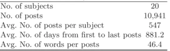
Table 1: Summary of the test data
No. of subjects 20
No. of posts 10,941
Avg. No. of posts per subject 547 Avg. No. of days from first to last posts 881.2 Avg. No. of words per posts 46.4
measures characteristic attitudes and symptoms of depression. Each question has 4 possible answers, numbered from 0 to 3, and is useful to assess the presence of feelings like sadness, pessimism, loss of energy, etc. For example, the question 3 is as follows:
Question 3. Past Failure: 0. I do not feel like a failure.
1. I have failed more than I should have. 2. As I look back, I see a lot of failures. 3. I feel I am a total failure as a person.
Therefore, this task aimed at exploring the viability of automatically esti-mating the severity of multiple symptoms associated with depression. Given the user’s history of postings, the algorithms had to estimate the user’s response to each individual question.
It is worth mentioning that for this task, no training data was provided and therefore, only the raw (unlabeled) test set used to evaluate the performance of all participants was provided. To build this test set, questionnaires filled by Reddit4users were collected together with their history of postings. User’s posts were collected right after he/she filled the BDI questionnaire. The questionnaires filled by the users were then used as the ground truth to assess the quality of the responses given by the participating systems. The details of the built test set are presented in Table 1.
2.1 Evaluation Metrics
In order to assess the quality of questionnaires filled by the systems, four metrics were used:
– Hit Rate (HR). This measure computes the ratio of cases where the automatic questionnaire has exactly the same answer as the real questionnaire. For example, an automatic questionnaire with 5 matches gets an HR equal to
5 21.
5
– Closeness Rate (CR). This measure takes into account that the answers of the BDI questionnaire represent an ordinal scale. For example, imagine that the 4 https://www.reddit.com/
real user answered option 0. A system, S1, whose answer was option 3 should be penalized more than a system S2 whose answer was 1. For each questioni, the absolute difference (ad) between the real and the automated answer (e.g. |0−3|= 3 and|0−1|= 1 for S1 and S2, respectively) it is computed and next, this absolute difference is normalized as follows:CRi= 3−3adi.
6
Finally, theCRi for each question is averaged to obtain the final effectiveness score, i.e.CR= 1
21
21
i=1CRi.
– Difference between Overall Depression Levels (DODL). The previous mea-sures assess the systems’ ability to answer each question. This measure, instead, does not look at question-level hits or differences but computes the overall depression level (sum of all the answers) for the real and automated questionnaire and next, the absolute difference (ad overall) between the real and the automated score is computed. In the BDI, depression level is an integer between 0 and 63 and thus, DODL is normalized between 0 and 1 as follows:DODL= 63−ad overall63 .
– Depression Category Hit Rate (DCHR). In the psychological domain, it is customary to associate depression levels with the following categories:
minimal (depression levels 0-9) mild (depression levels 10-18) moderate (depression levels 19-29) severe (depression levels 30-63)
This measure consists of computing the fraction of cases where the automated questionnaire led to a depression category that is equivalent to the depression category obtained from the real questionnaire.
Finally, for the first three measures, results were reported using the average over all the users and were referred to asAHR,ACR andADODL.
3
Our approach
To carry out this task, we trained a binary text classifier to detect “depressed” users and then we use its confidence values to estimate the user’s clinical depression level by completing the BDI questionnaire. We decided to use a text classifier that has shown remarkable performance on early depression detection and was firstly introduced in [3]. Thus, subsection 3.1 briefly introduces the used classifier, called SS3, and then subsection 3.2 describes how questionnaires were actually filled in.
3.1 The SS3 text classifier
As it is described in more details in [3], SS3 first builds a dictionary of words for each category during the training phase, in which the frequency of each
word is stored. Then, using those word frequencies, and during the classification stage, it calculates a value for each word using a functiongv(w, c) to value words in relation to categories. gv takes a word w and a category c and outputs a number in the interval [0,1] representing the degree of confidence with which w is believed to exclusively belong toc, for instance, suppose categories C = {f ood, music, health, sports}, we could have:
gv(‘sushi’, f ood) = 0.85; gv(‘the’, f ood) = 0; gv(‘sushi’, music) = 0.09; gv(‘the’, music) = 0; gv(‘sushi’, health) = 0.50;gv(‘the’, health) = 0; gv(‘sushi’, sports) = 0.02;gv(‘the’, sports) = 0; Additionally, a vectorial version ofgvis defined as:
− →
gv(w) = (gv(w, c0), gv(w, c1), . . . , gv(w, ck))
whereci∈C (the set of all the categories). That is,−gv→is only applied to a word and it outputs a vector in which each component is the gv of that word for each categoryci. For instance, following the above example, we have:
gv(‘sushi’) = (0.85,0.09,0.5,0.02);gv(‘the’) = (0,0,0,0);
The vector −→gv(w) is called the “confidence vector of w”. Note that each categoryci is assigned a fixed position in−→gv. For instance, in the example above (0.85,0.09,0.5,0.02) is the confidence vector of the word “sushi” and the first position corresponds tof ood, the second tomusic, and so on. For those readers interested in how thegvfunction is actually computed, we highly recommend to read the SS3 original paper[3], since its equations are not given here to keep this paper shorter and simpler.
SS3 classification process can be thought of as a 2-phase process. In the first phase the input document is split into multiple blocks (e.g. paragraphs), then each block is in turn repeatedly divided into smaller units (e.g. sentences, words). Thus, the previously “flat” document is transformed into a hierarchy of blocks. In the second phase, thegvfunction is applied to each word to obtain the “level 0” confidence vectors, which then are reduced to level 1 confidence vectors by means of a level 0summary operator,⊕0. This reduction process is recursively propagated up to higher-level blocks, using higher-levelsummary operators,⊕j, until a singleconfidence vector,−→d, is generated for the whole input. Finally, the actual classification is performed based on the values of this singleconfidence vector,−→d, using some policy —for example, selecting the category with the higher
confidence value. Note that using these confidence vectors in the hierarchy of blocks, it is quite straightforward for SS3 to visually justify the classification if different blocks of the input are colored in relations to their values, as can be seeing on an live demo available at http://tworld.io/ss3 in which users can try out SS3 for topic categorization. This is quite relevant when it comes to health-care
Fig. 1: Diagram of the dep level computation process for subject 2827. As reader can notice, after processing all the subject’s writings, the finalconfidence value
(0.941) was mapped into its corresponding dep level (55).
systems, specialists should be able to manually analyze classified subjects and this type of visual tools could be really helpful.
We used theaddition as thesummary operators for generating theconfidence vectors for all the levels, .i.e ⊕j = addition for all j, which simplified the classification process to the summation of all words’−gv→vectors read so far, in symbols, for every subjects:
− → ds= w∈W Hs − → gv(w) (1)
whereW Hsis the subject’s writing history. Note that for this task,−→ds was a vectordpos, dnegwith only two components, one for the “depressed” class, dpos, and the other for the “non-depressed” one, dneg. In [3], early classification of subjects was carried out by analyzing how thisconfidence vector changed over time (i.e. as more posts were processed).
3.2 Filling in the BDI questionnaires
As mentioned in section 2, the task was quite difficult, since it was not a single “yes or no” problem but a problem involving multiple decisions, one for each one of the 21 questions. To make things even harder, no training data was released either. Fortunately, early depression detection is a task we had some previous experience working with in previous CLEF’s eRisk challenges[5][4][3]. Therefore,
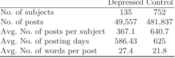
Table 2: Summary of the eRisk 2018 depression task’s dataset Depressed Control
No. of subjects 135 752
No. of posts 49,557 481,837 Avg. No. of posts per subject 367.1 640.7 Avg. No. of posting days 586.43 625 Avg. No. of words per post 27.4 21.8
we decided to train SS3 using the dataset for the eRisk 2018 depression detection task[8] (details are given in Table 2). Additionally, we used the same hyper-parameters used in [3], i.e. λ=ρ= 1 andσ= 0.455, for which SS3 showed to have state-of-the-art performance on depression detection.
However, the main problem was deciding how to turn this trained “yes or no” classifier into a classifier capable of filling BDI questionnaires. We came up with the idea of using theconfidence vector,−→d in Equation 1, to somehow infer a BDI depression level between 0 and 63. To achieve this, first, we converted the
confidence vector into a singleconfidence value (cv) normalized between 0 and 1, by applying the following equation:
cv=dpos−dneg
dpos (2)
Then, after SS3 classified a subject, the obtainedcvvalue was mapped into a region/category c, one for each BDI depression category (c∈ {0,1,2,3}). This was carried out by the following equation:
c=cv×4 (3)
And finally, the subject depression level was predicted by mapping the per-centage ofcvleft inside the predictedcregion to its corresponding BDI depression level range (e.g. (0.5,0.75]−→[19,29] for c= 2 = “moderate depression”) by computing the following:
dep level=minc+(maxc−minc+ 1)×(cv×4−c) (4) Wheremincandmaxc are the lower and upper bound for categoryc, respectively (e.g. 19 and 29 for “moderate depression” category).
In order to clarify the above process, we will illustrate it with the example shown in Figure 1. First, SS3 processed the entire writing history computing the
confidence value (given by Equation 2) and then, the finalcvvalue (0.941) was used to predict the depression category, “severe depression” (c= 3), by using the
Equation 3. Finally, the depression level was computed by the mapping given by Equation 4, as follows: dep level= 30 +(63−30 + 1)×(0.941×4−3) = 30 +34×(3.764−3) = 30 +34×0.764 = 30 + 25 =55 (5)
At this point we have transformed the output of SS3 from a 2-dimensional vector,d, into a BDI depression level (a value from 0 to 63). However we have not covered yet how to actually answer the 21 questions in the BDI questionnaire using thisdepression level. Regardless the method, we decided that for all those users whosedep levelwas less or equal to 0, all the BDI questions were answered with 0. For the other users we applied different methods since every participating team was allowed to use up to five different models (called “runs”) to carry out the task. Thus, we use five different methods to accomplish this task, as described below:
– UNSLA: using the predicteddep level our model filled the questionnaires answering the answer numberdep level21 on each question. If this division had a remainder, the remainder points were randomly scatter so that the sum of all the answers always matched the predicted depression level given by SS3.
– UNSLB: this time, only the predicted category,c, was used. Our model filled the questionnaire randomly in such a way that the final depression level always matched the predicted category,c. Compared to the following three ones, these two models were the ones with the worst performance.
– UNSLC: this model, and the following, were more question-centered. Once again, as in UNSLA, our model filled the questionnaires answering the expected number derived from the predicted depression level (dep level21 ). But this time, answering this number only on questions for which a “textual hint” for a possible answer was found in the user’s writings, and randomly and uniformly answered between 0 anddep level21 otherwise. To find this “textual hint”, our model split the user’s writings into sentences and searched for the co-occurrence of the words “I” or “my” with at least one word matching a regular expression specially crafted for each question.7This method obtained the best AHR (41.43%) and the second-best DCHR (40%).
– UNSLD: the same as the previous one, but not using the “textual hints”, i.e. always answering every question randomly and uniformly between 0 and dep level
21 . This model was mainly used only with the goal of measuring the actual impact of using these “textual hints” to decide which questions should be answerd with the expected answer (dep level
21 ).
7 e.g. “(sad)|(unhappy)” for question 1, “(future)|(work out)” for question 2, “fail\w*” for question 3, “(pleasure)|(enjoy)” for question 4, etc.
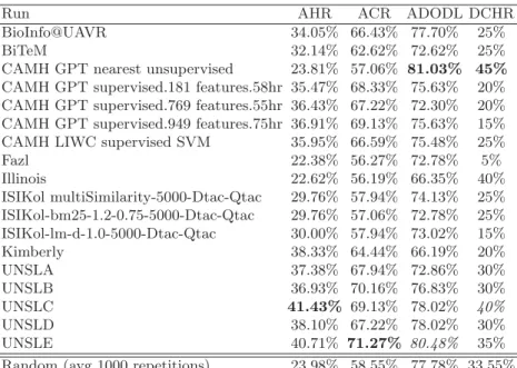
Table 3: Results for eRisk 2019 Task 3.
Run AHR ACR ADODL DCHR
BioInfo@UAVR 34.05% 66.43% 77.70% 25%
BiTeM 32.14% 62.62% 72.62% 25%
CAMH GPT nearest unsupervised 23.81% 57.06% 81.03% 45% CAMH GPT supervised.181 features.58hr 35.47% 68.33% 75.63% 20% CAMH GPT supervised.769 features.55hr 36.43% 67.22% 72.30% 20% CAMH GPT supervised.949 features.75hr 36.91% 69.13% 75.63% 15% CAMH LIWC supervised SVM 35.95% 66.59% 75.48% 25%
Fazl 22.38% 56.27% 72.78% 5% Illinois 22.62% 56.19% 66.35% 40% ISIKol multiSimilarity-5000-Dtac-Qtac 29.76% 57.94% 74.13% 25% ISIKol-bm25-1.2-0.75-5000-Dtac-Qtac 29.76% 57.06% 72.78% 25% ISIKol-lm-d-1.0-5000-Dtac-Qtac 30.00% 57.94% 73.02% 15% Kimberly 38.33% 64.44% 66.19% 20% UNSLA 37.38% 67.94% 72.86% 30% UNSLB 36.93% 70.16% 76.83% 30% UNSLC 41.43% 69.13% 78.02% 40% UNSLD 38.10% 67.22% 78.02% 30% UNSLE 40.71% 71.27% 80.48% 35%
Random (avg 1000 repetitions) 23.98% 58.55% 77.78% 33.55%
– UNSLE: the same as previous one, but this time not using a uniform distri-bution. More precisely, from the overall depression level predicted by SS3, once again the expected answer was computed (dep level
21 ) and, depending
on the value of the expected answer, actual answers were given using the following probability distributions:
P(0|0) = 0.9;P(1|0) = 0.1;P(2|0) = 0;P(3|0) = 0; P(0|1) = 0.2;P(1|1) = 0.6;P(2|1) = 0.1;P(3|1) = 0.1; P(0|2) = 0.15;P(1|2) = 0.25;P(2|2) = 0.5;P(3|2) = 0.1;
P(0|3) = 0.1;P(1|3) = 0.2;P(2|3) = 0.3;P(3|3) = 0.4;
whereP(A|B) means the “probability of answering A given that the expected answer is B”. Note that, unlike uniform distribution (used in UNSLD), when using these probability distributions the expected answer is more likely to be selected over the other ones. This model obtained the best ACR (71.27%) and the second-best AHR (40.71%) and ADODL (80.48%, best was only 0.54% above).
4
Evaluation Results
The task’s results are shown in Table 3. As mentioned above, we obtained the best AHR (41.43%) and ACR (71.27%), and the second-best ADODL (80.48%) and
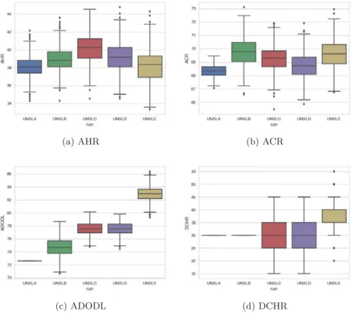
(a) AHR (b) ACR
(c) ADODL (d) DCHR
Fig. 2: Box plots for each measure and run.
DCHR (40%), best DCHR and ADODL were obtained by CAMH[1]. However, since most of our models’ answers are stochastically generated, it implies that all of these measures are also stochastically generated.8 The natural question in cases like this is “How do we know these results properly represent our models performance and we did not obtained them just by pure chance?”. In order to clarify this, once the eRisk finished and the golden truth was released, we run each model 1000 times and calculated the values for AHR, ACR, ADODL and DCHR each time.9 After this process finished, we ended up with a sample of 1000 values for each measure and model, which we then used to produce the box plots shown in Figure 2. Analyzing both the values in the table and the box plots one can notice that, in fact, when we participated we had a little bit of bad luck, specially for UNSLE’s ADODL, since one can see in Figure 2c that the actual 8 Only ADODL and DCHR for UNSLA and DHR for UNSLB are deterministically
determined bydepressionlevelandc.
value we obtained (80.84%) is almost a lower bound outlier. Another important thing that can be seen in Figure 2a is that the use of “textual hints”, in UNSLC, really improved the Average Hit Rate (AHR) but did not impact on the other measures (as seen in the other figures). In Figure 2c we can see that UNSLE was considerably the best method to estimate the overall depression level since its ADODL takes values within a range that is quite above the others. Additionally, another important aspect is that, looking at the range of values each method takes, for the different measures, in Figure 2, we can see that the obtained values would be among the best ones, even in the worst cases (compared against the other participant’s).
5
Conclusions and Future Work
In previous scenarios, machine learning models have shown that, in fact, language usage can provide strong evidence in detecting depressive people, since these models have to learn to characterize depression through language use. The work presented in this article is a first step towards measuring finer grain relationships between these both aspects, namely, we studied how the language usage could be connected with theseverity level of depression. We tested our proposal by participating in the eRisk 2019 T3 task. Obtained results were quite promising and showed us that could be a strong, and somewhat direct, relationship within these both aspects —i.e. it could really be a relationship between how subjects write, what words they use, and the actual depression level they have. Finally, since all the methods we used are based on the depression level predicted by SS3, results also showed us that SS3 correctly inferred the depression level (calculated by Equation 4) from the textual evidence accumulated while processing the user’s writings, i.e. SS3 correctly valued words in relation to each category (depressed and non-depressed).
For future work we will try to get access to a bigger test set, since, although results were quite promising, more data is needed to draw better and more robust conclusions. Additionally, since at the time this paper was written information regarding the other participant’s models were not yet given, once this information is released, we plan to make a better and more qualitative analysis of the results by comparing our models against the other ones in more details. In fact, once we have access to this information, we also plan to explore different model variations to improve our predicted depression level.
References
1. Abed-Esfahani, P., Howard, D., Maslej, M., Patel, S., Mann, V., Goegan, S., French, L.: Transfer learning for depression: Early detection and severity prediction from social media postings. In: Experimental IR Meets Multilinguality, Multimodality, and Interaction. 10th International Conference of the CLEF Association, CLEF 2019. Springer International Publishing, Lugano, Switzerland (2019)
2. Beck, A.T., Ward, C.H., Mendelson, M., Mock, J., Erbaugh, J.: An inventory for measuring depression. Archives of general psychiatry4(6), 561–571 (1961)
3. Burdisso, S.G., Errecalde, M., y G´omez, M.M.: A text classification framework for simple and effective early depression detection over so-cial media streams. Expert Systems with Applications 133, 182 – 197 (2019). https://doi.org/10.1016/j.eswa.2019.05.023,http://www.sciencedirect. com/science/article/pii/S0957417419303525
4. Errecalde, M.L., Villegas, M.P., Funez, D.G., Ucelay, M.J.G., Cagnina, L.C.: Tempo-ral variation of terms as concept space for early risk prediction. In: Experimental IR Meets Multilinguality, Multimodality, and Interaction. 8th International Conference of the CLEF Association, CLEF 2017. Springer International Publishing, Dublin, Ireland (2017)
5. Funez, D.G., Ucelay, M.J.G., Villegas, M.P., Burdisso, S.G., Cagnina, L.C., Montes-y G´omez, M., Errecalde, M.L.: UNSL’s participation at erisk 2018 lab. In: Experi-mental IR Meets Multilinguality, Multimodality, and Interaction. 9th International Conference of the CLEF Association, CLEF 2018. Springer International Publishing, Avignon, France (2018)
6. Losada, D.E., Crestani, F.: A test collection for research on depression and language use. In: International Conference of the Cross-Language Evaluation Forum for European Languages. pp. 28–39. Springer (2016)
7. Losada, D.E., Crestani, F., Parapar, J.: erisk 2017: Clef lab on early risk prediction on the internet: Experimental foundations. In: International Conference of the Cross-Language Evaluation Forum for European Languages. pp. 346–360. Springer (2017)
8. Losada, D.E., Crestani, F., Parapar, J.: Overview of erisk: Early risk prediction on the internet. In: International Conference of the Cross-Language Evaluation Forum for European Languages. pp. 343–361. Springer (2018)
9. Losada, D.E., Crestani, F., Parapar, J.: Overview of eRisk 2019: Early Risk Pre-diction on the Internet. In: Experimental IR Meets Multilinguality, Multimodality, and Interaction. 10th International Conference of the CLEF Association, CLEF 2019. Springer International Publishing, Lugano, Switzerland (2019)
10. National Center for Health Statistics: Mortality in the United States, 2017.https: //www.cdc.gov/nchs/products/databriefs/db328.htm(2019), [Online; accessed 13-April-2019]
11. World Health Organization: Preventing suicide: a global imperative. WHO (2014) 12. World Health Organization: Depression and other common mental disorders: global