Édouard Bonnet
Univ Lyon, CNRS, ENS de Lyon, Université Claude Bernard Lyon 1, LIP UMR5668, France [email protected]
Nidhi Purohit
Univ Lyon, CNRS, ENS de Lyon, Université Claude Bernard Lyon 1, LIP UMR5668, France [email protected]
Abstract
A resolving setS of a graphGis a subset of its vertices such that no two vertices ofGhave the same distance vector toS. TheMetric Dimensionproblem asks for a resolving set of minimum size, and in its decision form, a resolving set of size at most some specified integer. This problem is NP-complete, and remains so in very restricted classes of graphs. It is also W[2]-complete with respect to the size of the solution. Metric Dimensionhas proven elusive on graphs of bounded treewidth. On the algorithmic side, a polytime algorithm is known for trees, and even for outerplanar graphs, but the general case of treewidth at most two is open. On the complexity side, no parameterized hardness is known. This has led several papers on the topic to ask for the parameterized complexity of Metric Dimensionwith respect to treewidth.
We provide a first answer to the question. We show thatMetric Dimensionparameterized by the treewidth of the input graph is W[1]-hard. More refinedly we prove that, unless the Exponential Time Hypothesis fails, there is no algorithm solvingMetric Dimensionin timef(pw)no(pw)on n-vertex graphs of constant degree, with pw the pathwidth of the input graph, andfany computable function. This is in stark contrast with an FPT algorithm of Belmonte et al. [SIAM J. Discrete Math. ’17] with respect to the combined parameter tl + ∆, where tl is the tree-length and ∆ the maximum-degree of the input graph.
2012 ACM Subject Classification Theory of computation→Graph algorithms analysis; Theory of computation→Fixed parameter tractability
Keywords and phrases Metric Dimension, Treewidth, Parameterized Hardness
Digital Object Identifier 10.4230/LIPIcs.IPEC.2019.5
Related Version A full version of the paper is available athttps://arxiv.org/abs/1907.08093.
1
Introduction
TheMetric Dimensionproblem has been introduced in the 1970s independently by Slater
[22] and by Harary and Melter [13]. Given a graphGand an integerk,Metric Dimension asks for a subsetS of vertices ofGof size at mostksuch that every vertex ofGis uniquely determined by its distances to the vertices ofS. Such a setS is called aresolving set, and a resolving set of minimum-cardinality is called ametric basis. The metric dimension of graphs finds application in various areas including network verification [2], chemistry [4], and robot navigation [18].
Metric Dimension is an entry of the celebrated book on intractability by Garey and
Johnson [12] where the authors show that it is NP-complete. In factMetric Dimension remains NP-complete in many restricted classes of graphs such as planar graphs [6], split, bipartite, co-bipartite graphs, and line graphs of bipartite graphs [9], interval graphs of diameter two [11], permutation graphs of diameter two [11], and in a subclass of unit disk graphs [16]. Furthermore Metric Dimension cannot be solved in subexponential-time unless 3-SATcan [1]. On the positive side, the problem is polynomial-time solvable on trees [22, 13, 18]. Diaz et al. [6] generalize this result to outerplanar graphs. Fernau et al. [10]
© Édouard Bonnet and Nidhi Purohit;
give a polynomial-time algorithm on chain graphs. Epstein et al. [9] show thatMetric
Dimension (and even its vertex-weighted variant) can be solved in polynomial time on
co-graphs and forests augmented by a constant number of edges. Hoffmann et al. [15] obtain a linear algorithm on cactus block graphs.
Hartung and Nichterlein [14] prove thatMetric Dimensionis W[2]-complete (paramet-erized by the size of the solutionk) even on subcubic graphs. Therefore an FPT algorithm solving the problem is unlikely. However Foucaud et al. [11] give an FPT algorithm with respect tokon interval graphs. This result is later generalized by Belmonte et al. [3] who obtain an FPT algorithm with respect to tl + ∆ (where tl is the tree-length and ∆ is the maximum-degree of the input graph), implying one for parameter tl +k. Indeed interval graphs, and even chordal graphs, have constant tree-length. Hartung and Nichterlein [14] presents an FPT algorithm parameterized by the vertex cover number, Eppstein [8], by the max leaf number, and Belmonte et al. [3], by the modular-width (a larger parameter than clique-width).
The complexity of Metric Dimensionparameterized by treewidth is quite elusive. It is discussed [8] or raised as an open problem in several papers [3, 6]. On the one hand, it was not known, prior to our paper, if this problem is W[1]-hard. On the other hand, the complexity of Metric Dimensionin graphs of treewidth at most two is still an open question.
1.1
Our contribution
We settle the parameterized complexity of Metric Dimensionwith respect to treewidth. We show that this problem is W[1]-hard, and we rule out, under the Exponential Time Hypothesis (ETH), an algorithm running inf(tw)|V(G)|o(tw), whereGis the input graph, tw its treewidth, andf any computable function. Our reduction even shows that an algorithm in timef(pw)|V(G)|o(pw) is unlikely on constant-degree graphs, for the larger parameter pathwidth pw. This is in stark contrast with the FPT algorithm of Belmonte et al. [3] for the parameter tl + ∆ where tl is the tree-length and ∆ is the maximum-degree of the graph. We observe that this readily gives an FPT algorithm for ctw + ∆ where ctw is the connected treewidth, since ctw>tl. This unravels an interesting behavior of Metric Dimension, at least on bounded-degree graphs: usual tree-decompositions are not enough for efficient solving. Instead one needs tree-decompositions with an additional guarantee that the vertices of a same bag are at a bounded distance from each other.
As our construction is quite technical, we chose to introduce an intermediate problem dubbedk-Multicolored Resolving Setin the reduction fromk-Multicolored
Inde-pendent SettoMetric Dimension. The first half of the reduction, fromk-Multicolored
Independent Settok-Multicolored Resolving Set, follows a generic and standard
recipe to design parameterized hardness with respect to treewidth. The main difficulty is to design an effectivepropagation gadget with a constant-size left-right cut. The second half brings some new local attachments to the produced graph, to bridge the gap between
k-Multicolored Resolving SetandMetric Dimension. Along the way, we introduce
a number of gadgets: edge, propagation, forced set, forced vertex. They are quite stream-lined and effective. Therefore, we believe these building blocks may help in designing new reductions forMetric Dimension.
1.2
Organization of the paper
In Section 2 we introduce the definitions, notations, and terminology used throughout the paper. In Section 3 we present the high-level ideas to establish our result. We define
thek-Multicolored Resolving Setproblem which serves as an intermediate step for
our reduction. In Section 4 we design a parameterized reduction from the W[1]-complete
k-Multicolored Independent Set tok-Multicolored Resolving Set
parameter-ized by treewidth. In Section 5 we show how to transform the produced instances of
k-Multicolored Resolving Set toMetric Dimension-instances (while maintaining
bounded treewidth). Due to space constraints, the proofs of lemmas marked with a star are deferred to the long version (in appendix).
2
Preliminaries
We denote by [i, j] the set of integers{i, i+ 1, . . . , j−1, j}, and by [i] the set of integers [1, i]. IfX is a set of sets, we denote by∪X the union of them.
2.1
Graph notations
All our graphs are undirected and simple (no multiple edge nor self-loop). We denote by V(G), respectively E(G), the set of vertices, respectively of edges, of the graph G. For S⊆V(G), we denote theopen neighborhood (or simplyneighborhood) ofS byNG(S), i.e.,
the set of neighbors ofS deprived ofS, and theclosed neighborhood ofS byNG[S], i.e., the
setNG(S)∪S. For singletons, we simplifyNG({v}) intoNG(v), andNG[{v}] intoNG[v]. We
denote byG[S] the subgraph ofGinduced byS, andG−S:=G[V(G)\S]. ForS⊆V(G) we denote byS the complementV(G)\S. For A, B ⊆V(G), E(A, B) denotes the set of edges inE(G) with one endpoint inAand the other one inB.
The length of a path in an unweighted graph is simply the number of edges of the path. For two verticesu, v∈V(G), we denote by distG(u, v), the distance betweenuandv inG,
that is the length of the shortest path between uand v. The diameter of a graph is the longest distance between a pair of its vertices. The diameter of a subsetS⊆V(G), denoted by diamG(S), is the longest distance between a pair of vertices inS. Note that the distance
is taken inG,not in G[S]. In particular, whenGis connected, diamG(S) is finite for every
S. Apendant vertex is a vertex with degree one. A vertexuispendant tov ifv is the only neighbor ofu. Two distinct verticesu, v such that N(u) =N(v) are calledfalse twins, and true twins ifN[u] =N[v]. In particular, true twins are adjacent. In all the above notations with a subscript, we omit it whenever the graph is implicit from the context.
2.2
Exponential Time Hypothesis, FPT reductions, and W[1]-hardness
TheExponential Time Hypothesis (ETH) is a conjecture by Impagliazzo et al. [17] asserting that there is no 2o(n)-time algorithm for3-SATon instances withnvariables. Lokshtanov
et al. [20] survey conditional lower bounds under the ETH.
A standard use of an FPT reduction is to derive conditional lower bounds: if a problem (Π, κ) is thought not to admit an FPT algorithm, then an FPT reduction from (Π, κ) to (Π0, κ0) indicates that (Π0, κ0) is also unlikely to admit an FPT algorithm. We refer the reader to the textbooks [7, 5] for a formal definition of W[1]-hardness. For the purpose of this paper, we will just state that W[1]-hard are parameterized problems that are unlikely to be FPT, and that the following problem is W[1]-complete even when all theVi have the
k-Multicolored Independent Set(k-MIS) Parameter: k
Input: An undirected graphG, an integer k, and (V1, . . . , Vk) a partition ofV(G). Question: Is there a setI⊆V(G) such that|I∩Vi| = 1 for everyi∈[k], andG[I] is
edgeless?
Every parameterized problem thatk-Multicolored Independent Set FPT-reduces to is W[1]-hard. Our paper is thus devoted to designing an FPT reduction from k
-Multicolored Independent Set to Metric Dimension parameterized by tw. Let
us observe that the ETH implies that one (equivalently, every) W[1]-hard problem is not in the class of problems solvable in FPT time (FPT6=W[1]). Thus if we admit that there is no subexponential algorithm solving3-SAT, thenk-Multicolored Independent Setis not solvable in timef(k)|V(G)|O(1). Actually under this stronger assumption,k
-Multicolored Independent Setis not solvable in timef(k)|V(G)|o(k). A concise proof of that fact can be found in the survey on the consequences of ETH [20].
2.3
Metric dimension, resolved pairs, distinguished vertices
A pair of vertices{u, v} ⊆V(G) is said to beresolved by a setS if there is a vertexw∈S such that dist(w, u)6= dist(w, v). A vertex uis said to bedistinguished by a setS if for any w∈V(G)\ {u}, there is a vertexv∈S such that dist(v, u)6= dist(v, w). Aresolving set of a graphGis a setS⊆V(G) such that every two distinct verticesu, v ∈V(G) are resolved byS. Equivalently, a resolving set is a set S such that every vertex ofGis distinguished byS. ThenMetric Dimensionasks for a resolving set of size at most some thresholdk. Note that a resolving set of minimum size is sometimes called ametric basisforG.
Metric Dimension(MD) Parameter: tw(G)
Input: An undirected graphGand an integer k.
Question: DoesGadmit a resolving set of size at mostk?
Here we anticipate on the fact that we will mainly considerMetric Dimension paramet-erized by treewidth. Henceforth we sometimes use the notation Π/tw to emphasize that Π is not parameterized by the natural parameter (size of the resolving set) but by the treewidth of the input graph.
3
Outline of the W[1]-hardness proof of Metric Dimension/tw
We will show the following.ITheorem 1. Unless the ETH fails, there is no computable function f such that Metric Dimensioncan be solved in timef(pw)no(pw) on constant-degree n-vertex graphs.
We first prove that the following generalized version of Metric Dimensionis W[1]-hard.
k-Multicolored Resolving Set(k-MRS) Parameter: tw(G)
Input: An undirected graph G, an integer k, a set X of q disjoint subsets of V(G): X1, . . . , Xq, and a setP of pairs of vertices ofG: {x1, y1}, . . . ,{xh, yh}.
Question: Is there a setS⊆V(G) of sizeqsuch that (i) for everyi∈[q],|S∩Xi| = 1, and
(ii) for everyp∈[h], there is ans∈S satisfying distG(s, xp)6= distG(s, yp)?
In words, in this generalized version the resolving set is made by picking exactly one vertex in each set of X, and not all the pairs should be resolved but only the ones in a prescribed setP. We call critical pair a pair of P. In the context of k-Multicolored
Resolving Set, we calllegal set a set which satisfies the former condition, andresolving set a set which satisfies the latter. Thus a solution fork-Multicolored Resolving Set is a legal resolving set.
The reduction from k-Multicolored Independent Setstarts with a well-established trick to show parameterized hardness by treewidth. We create m “empty copies” of the k-MIS-instance (G, k,(V1, . . . , Vk)), wherem:=|E(G)|and t:=|Vi|. We force exactly one
vertex in each color class of each copy to be in the resolving set, using the setX. In each copy, we introduce an edge gadget for a single (distinct) edge ofG. Encoding an edge of k-MISin thek-MRS-instance is fairly simple: we build a pair (ofP) which is resolved by every choice but the one selecting both its endpoints in the resolving set. We now need to force a consistent choice of the vertex chosen inVi over all the copies. We thus design a
propagation gadget. A crucial property of the propagation gadget, for the pathwidth of the constructed graph to be bounded, is that it admits a cut of sizeO(k) disconnecting one copy from the other. Encoding a choice inVi in the distances to four special vertices, calledgates,
we manage to build such a gadget with constant-size “left-right” separator per color class. This works by introducingtpairs (ofP) which are resolved by the south-west and north-east gates but not by the south-east and north-west ones. Then we link the vertices of a copy ofVi in a way that the higher their index, the more pairs they resolve in the propagation
gadget to their left, and the fewer pairs they resolve in the propagation gadget to their right. We then turn to the actual Metric Dimensionproblem. We design a gadget which simulates requirement (i) by forcing a vertex of a specific setX in the resolving set. This works by introducing two pairs that are only resolved by vertices ofX. We attach this new gadget, calledforcing set gadget, to all thekcolor classes of themcopies. Finally we have to make sure that a candidate solution resolves all the pairs, and not only the ones prescribed byP. For that we attach two adjacent “pendant” vertices to strategically chosen vertices. One of these two vertices have to be in the resolving set since they are true twins, hence not resolved by any other vertex. Then everything is as if the unique common neighborv of the true twins was added to the resolving set. Therefore we can perform this operation as long asv does not resolve any of the pairs ofP.
To facilitate the task of the reader, henceforth we stick to the following conventions: Indexi∈[k] ranges over thek rowsof the(G)MD-instance or color classes of k-MIS. Indexj∈[m] ranges over themcolumns of the(G)MD-instance or edges of k-MIS. Indexγ∈[t], ranges over thetvertices of a color class.
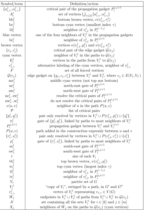
We invite the reader to look up Table 1 when in doubt about a notation/symbol relative to the construction.
4
Parameterized hardness of
k-Multicolored Resolving Set/tw
In this section, we give an FPT reduction from the W[1]-complete k-Multicolored
Independent Set to k-Multicolored Resolving Set parameterized by treewidth.
More precisely, given ak-Multicolored Independent Set-instance (G, k,(V1, . . . , Vk))
we produce in polynomial-time an equivalentk-Multicolored Resolving Set-instance (G0, k0,X,P) whereG0 has pathwidth (hence treewidth)O(k).
4.1
Construction
Let (G, k,(V1, . . . , Vk)) be an instance of k-Multicolored Independent Set where
(V1, . . . , Vk) is a partition of V(G) and Vi := {vi,γ | 16 γ 6 t}. We arbitrarily number
4.1.1
Overall picture
We start with a high-level description of thek-MRS-instance (G0, k0,X,P). For each color classVi, we introducemcopiesVi1, . . . , V
j
i , . . . , Vimof aselector gadget toG0. Each set V j i
is added toX, so a solution has to pick exactly one vertex within each selector gadget. One can imagine the vertex-setsV1
i , . . . , Vim to be aligned on thei-th row, with V j
i occupying
thej-th column(see Figure 1). EachVij hastvertices denoted byvi,j1, vji,2, . . . , vji,t, where eachvi,γj “corresponds” tovi,γ∈Vi. We makev
j i,1v
j i,2. . . v
j
i,t a path witht−1 edges.
For each edge ej ∈E(G), we insert anedge gadget G(ej) containing a pair of vertices
{cj, c0j} that we add toP. GadgetG(ej) is attached toVij andV j
i0, whereej ∈E(Vi, Vi0).
The edge gadget is designed in a way that the only legal sets that do not resolve {cj, c0j}
are the ones that precisely pickvi,γj ∈Vij andvji0,γ0 ∈V j
i0 such thatej =vi,γvi0,γ0. We add a
propagation gadgetPij,j+1 between two consecutive copiesVij andVij+1, where the indices in the superscript are taken modulom. The role of the propagation gadget is to ensure that the choices in eachVij (j∈[m]) corresponds to the same vertex in Vi.
V1 1 V12 V13 V14 V15 V16 V1 2 V22 V23 V24 V25 V26 V31 V32 V33 V34 V35 V36 P11,2 P12,3 P13,4 P14,5 P15,6 P21,2 P22,3 P23,4 P24,5 P25,6 P31,2 P32,3 P33,4 P34,5 P35,6 P16,1 P26,1 P36,1 G(e1) G(e2) G(e3) G(e4) G(e5) G(e6)
Figure 1The overall picture withk= 3 color classes,t= 5 vertices per color class,m= 6 edges, e1=v1,3v2,4,e2=v1,4v2,1,e3=v1,5v3,1, etc. The dashed lines on the left and right symbolize that
the construction is cylindrical.
The intuitive idea of the reduction is the following. We say that a vertex ofG0 isselected
if it is put in the resolving set ofG0, a tentative solution. The propagation gadgetPij,j+1 ensures a consistent choice among themcopies V1
i , . . . , Vim. The edge gadget ensures that
the selected vertices ofG0 correspond to an independent set in the original graphG. If both the endpoints of an edgeej are selected, then the pair{cj, c0j}is not resolved. We now detail
4.1.2
Selector gadget
For eachi∈[k] andj∈[m], we add toG0 a path ont−1 edgesvji,1, vi,j2, . . . , vi,tj , and denote this set of vertices byVij. Each vi,γj correspondstovi,γ ∈Vi. We callj-th column the set
S
i∈[k]V
j
i , andi-th row, the set
S j∈[m]V j i. We set X :={V j i }i∈[k],j∈[m]. By definition of k-Multicolored Resolving Set, a solutionS has to satisfy that for everyi∈[k], j∈[m], |S∩Vij|= 1. We call legal set a setS of sizek0=kmthat satisfies this property. We call consistent set a legal set S which takes the “same” vertex in each row, that is, for every i∈[k], for every pair (vi,γj , vi,γj00)∈(S∩V
j
i )×(S∩V j0
i ), thenγ=γ0.
4.1.3
Edge gadget
For each edgeej=vi,γvi0,γ0 ∈E(G), we add an edge gadgetG(ej) in thej-th column ofG0.
G(ej) consists of a path on three vertices: cjgjc0j. The pair{cj, c0j}is added to the list of
critical pairs P. We link both vji,γ andvji0,γ0 togj by a private path1 of lengtht+ 2. We
link the at least two and at most four verticesvi,γj −1, vji,γ+1, vij0,γ0−1, v j
i0,γ0+1 (whenever they
exist) tocj by a private path of lengtht+ 2. This defines at most six paths fromVij∪V j i0 to
G(ej). Let us denote byWj the at most six endpoints of these paths inV j
i ∪V
j
i0. For each
v∈Wj, we denote byP(v, j) the path fromv toG(ej). We setEij :=
S
v∈Wj∩Vij
P(v, j) and Eij0 :=Sv∈W
j∩Vij0P(v, j). We denote by Xj the set of the at most six neighbors of Wj on
the paths toG(ej). Henceforth we may refer to the vertices in someXj as thecyan vertices.
Individually we denote byeji,γ the cyan vertex neighbor ofvji,γ inP(vi,γj , j). We observe that for fixediandj,eji,γ exists for at most three values ofγ. We add an edge between two cyan vertices if their respective neighbors inVij are also linked by an edge (or equivalently, if they have consecutive “indicesγ”). These extra edges are useless in thek-MRS-instance, but will turn out useful in theMD-instance. See Figure 2 for an illustration of the edge gadget.
The rest of the construction will preserve that for every v ∈(Vij ∪Vij0)\ {v j i,γ, v
j i0,γ0},
dist(v, c0j) = dist(v, cj) + 2, and for each v ∈ {v j i,γ, v
j
i0,γ0}, dist(v, cj) = dist(v, gj) + 1 =
dist(v, c0j). In other words, the only two vertices of Vij∪Vij0 not resolving the critical pair
{cj, c0j}arev j
i,γ andv j
i0,γ0, corresponding to the endpoints ofej.
4.1.4
Propagation gadget
Between each pair (Vij, Vij+1), wherej+ 1 is taken modulom, we insert an identical copy of the propagation gadget, and we denote it byPij,j+1. It ensures that if the vertexvi,γj is in a legal resolving setS, then the vertex ofS∩Vij+1should be some vji,γ+10 withγ6γ0. The
cylindricity of the construction and the fact that exactly one vertex ofVij is selected, will therefore impose that the setS is consistent.
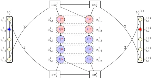
Pi,j,j+1 comprises four vertices swji, seji, nwij, neji, calledgates, and a setAji of 2tvertices aji,1, . . . , aji,t, αji,1, . . . , αji,t. We make bothaji,1ai,j2. . . aji,tandαji,1αji,2. . . αji,t a path witht−1 edges. For eachγ∈[t], we add the pair{aji,γ, αji,γ} to the set of critical pairsP. Removing the gates disconnectsAji from the rest of the graph.
We now describe how we link the gates to Vij, Vij+1, andAji. We link vi,j1 (the “top” vertex ofVij) to swji andvi,tj (the “bottom” vertex ofVij) to nwji both by a path of length 2.
1 We use the expressionprivate path to emphasize that the different sources get a pairwise internally
V14 V4 2 V4 3 v14,1 v14,2 v14,3 v14,4 v14,5 e41,4 e4 1,5 g4 c4 c04 G(e4) 6 6 6 6 6
Figure 2The edge gadgetG(e4) withe4=v1,5v3,3. Weighted edges are short-hands for
subdivi-sions of the corresponding length. The edges between the cyan vertices will not be useful for the k-MRS-instance, but will later simplify the construction of theMD-instance.
We also linkvji,+11 to seji by a path of length 3, and vji,t+1 to neji by a path of length 2. Then we make nwji adjacent toaji,1and αi,j1, while we make neji adjacent toαji,1only. We make seji adjacent toaji,t andαji,t, while we make swji adjacent toaji,t only. Finally, we add an edge between neji and nwji, and between swji and seji. See Figure 3 for an illustration of the propagation gadgetPij,j+1 witht= 5.
vji,1 vji,2 vji,3 vji,4 vji,5 vi,j+11 vi,j+12 vi,j+13 vi,j+14 vi,j+15 Vij Vij+1 swji seji nwji neji 6|7 7|8 6|7 5|6 4|5 6|6 7|7 7|7 6|6 5|5 aji,1 αji,1 aji,2 αji,2 aji,3 αji,3 aji,4 αji,4 aji,5 αji,5 2 3 2 2
Figure 3The propagation gadgetPij,j+1. The critical pairs{aji,γ, αji,γ}are surrounded by thin dashed lines. The blue (resp. red) integer on a vertex ofAji is its distance to the blue (resp. red) vertex inVij(resp. Vij+1). Note that the blue vertex distinguishes the critical pairs below it, while the red vertex distinguishes critical pairs at its level or above.
Let us motivate the gadgetPij,j+1. One can observe that the gates neji and swji resolve the critical pairs of the propagation gadget, while the gates nwji and seji do not. Consider that the vertex added to the resolving set inVij is vji,γ. Its shortest paths to critical pairs belowit (that is, with index γ0 > γ) go through the gate swji, whereas its shortest paths to critical pairs at its level or above (that is, with indexγ06γ) go through the gate nwji. Thus vi,γj only resolves the critical pairs{aji,γ0, αi,γ0} withγ0 > γ. On the contrary, the vertex of
the resolving set inVij+1 only resolves the critical pairs {aji,γ0, α j
i,γ0} at its level or above.
This will force that its level isγ or below. Hence the vertices of the resolving inVij and Vij+1 should be such thatγ0>γ. Since there is also a propagation gadget betweenVim and V1
i , this circular chain of inequalities forces a global equality.
4.1.5
Wrapping up
We put the pieces together as described in the previous subsections. At this point, it is convenient to give names to the neighbors of Vij in the propagation gadgetsPij−1,j and Pij,j+1. We may refer to them asblue vertices (as they appear in Figure 4). We denote by tlji the neighbor ofvji,1 inPij−1,j, trij, the neighbor ofvji,1in Pij,j+1, blji, the neighbor ofvi,tj inPij−1,j, and brji, the neighbor ofvi,tj in Pij,j+1. We add the following edges and paths.
For any pairi, j such that the edgeej has an endpoint inVi, the vertices tlji,tr j i,bl j i,br j i
are linked togj by a private path of length the distance of their unique neighbor inV j i to
cj. We add an edge between seji and se j+1 i , and between nw j i and nw j+1 i (wherej+ 1 is
modulom). Finally, for everyej ∈E(Vi, Vi0), we add four paths between sej i,se j i0,nw j i,nw j i0
andgj∈ G(ej). More precisely, for eachi00∈ {i, i0}, we add a path fromgj to seji00 of length
dist(gj,sw j
i00)−4, and a path from gj to nw j
i00 of length dist(gj,nw j
i00)−4. These distances
are taken in the graph before we introduced the new paths, and one can observe that the length of these paths is at leastt. This finishes the construction.
4.2
Correctness of the reduction
We now check that the reduction is correct. We start with the following technical lemma. If a setX contains a pair that no vertex ofN(X) (that isN[X]\X) resolves, then no vertex outsideX can distinguish the pair.
ILemma 2. LetX be a subset of vertices, anda, b∈X be two distinct vertices. If for every vertexv∈N(X), dist(v, a) =dist(v, b), then for every vertex v /∈X, dist(v, a) =dist(v, b). Proof. Let vbe a vertex outside ofX. We further assume thatv is not inN(X), otherwise we can already conclude that it does not distinguish {a, b}. A shortest path from v to a, has to go through N(X). Let wa be the first vertex of N(X) met in this shortest
path from v to a. Similarly, let wb be the first vertex of N(X) met in a shortest path
fromv tob. Sincewa, wb ∈N(X), they satisfy dist(wa, a) = dist(wa, b) and dist(wb, a) =
dist(wb, b). Then, dist(v, a)6dist(v, wb) + dist(wb, a) = dist(v, wb) + dist(wb, b) = dist(v, b),
and dist(v, b) 6 dist(v, wa) + dist(wa, b) = dist(v, wa) + dist(wa, a) = dist(v, a). Thus
dist(v, a) = dist(v, b). J
We use the previous lemma to show that every vertex of a Vij only resolves critical pairs in gadgets it is attached to. This will be useful in the two subsequent lemmas.
ILemma 3(?). For any i∈[k],j∈[m], andv∈Vij,v does not resolve any critical pair outside ofPij−1,j, Pij,j+1 (where indices in the superscript are taken modulom), and{cj, c0j}.
The two following lemmas show the equivalences relative to the expected use of the edge and propagation gadgets. They will be useful in Sections 4.2.1 and 4.2.2.
ILemma 4 (?). A legal set S resolves the critical pair{cj, c0j} withej =vi,γvi0,γ0 if and
only if the vertexvji,γ i in V
j
i ∩S and the vertexv j i0,γ
i0 in V j
i0∩S satisfy (γ, γ0)6= (γi, γi0).
ILemma 5(?). A legal setSresolves all the critical pairs ofPij,j+1 if and only if the vertex vji,γ inVij∩S and the vertexvji,γ+10 inV
j+1
i ∩S satisfyγ6γ 0.
We can now prove the correctness of the reduction. The construction can be computed in polynomial time in|V(G)|, andG0 itself has size bounded by a polynomial in|V(G)|. We postpone checking that the pathwidth is bounded byO(k) to the end of the second step, where we produce an instance of MDwhose graph G00admitsG0 as an induced subgraph.
4.2.1
k-Multicolored Independent Set in
G
⇒
legal resolving set in
G
0 Let {v1,γ1, . . . , vk,γk} be a k-multicolored independent set in G. We claim that S := Sj∈[m]{v
j
1,γ1, . . . , v j
k,γk} is a legal resolving set inG
0 (of size km). The set S is legal by
construction. Since for everyi∈[k], and j∈[m], vi,γj i andv
j+1
i,γi are inS (j+ 1 is modulo m), all the critical pairs in the propagation gadgets are resolved byS, by Lemma 5. Since {v1,γ1, . . . , vk,γk} is an independent set inG, there is no ej =vi,γvi0,γ0 ∈E(G), such that (γ, γ0) = (γi, γi0). Thus every critical pair{cj, c0j} is resolved byS, by Lemma 4.
4.2.2
Legal resolving set in
G
0⇒
k-Multicolored Independent Set in
G
Assume that there is a legal resolving setS inG0. For everyi∈[k], for everyj∈[m], the vertexvji,γ(i,j)inVij∩Sand the vertexvi,γj+1(i,j+1)inVij+1∩S(j+1 is modulom) are such that γ(i, j)6γ(i, j+1), by Lemma 5. Thusγ(i,1)6γ(i,2)6. . .6γ(i, m−1)6γ(i, m)6γ(i,1), andγi:=γ(i,1) =γ(i,2) =. . .=γ(i, m−1) =γ(i, m). We claim that{v1,γ1, . . . , vk,γk}is a k-multicolored independent set inG. Indeed, there cannot be an edgeej=vi,γivi0,γi0 ∈E(G), since otherwise the critical pair{cj, c0j}is not resolved, by Lemma 4.5
Parameterized hardness of Metric Dimension/tw
In this section, we produce in polynomial time an instance (G00, k00) of Metric Dimension equivalent to (G0,X, km,P) of k-Multicolored Resolving Set. The graphG00 has also pathwidthO(k). Now, an instance is just a graph and an integer. There is no longerX and P to constrain and respectively loosen the “resolving set” at our convenience. This creates two issues: (1) the vertices outside the former setX can now be put in the resolving set, potentially yielding undesired solutions2 and (2) our candidate solution (when there is a k-multicolored independent set inG) may not distinguish all the vertices.
5.1
Construction
5.1.1
Forced set gadget
To deal with the issue (1), we introduce two new pairs of vertices for eachVij. The intention is that the only vertices resolving both these pairs simultaneously are precisely the vertices
2 Also, it is now possible to put two or more vertices of the sameVj
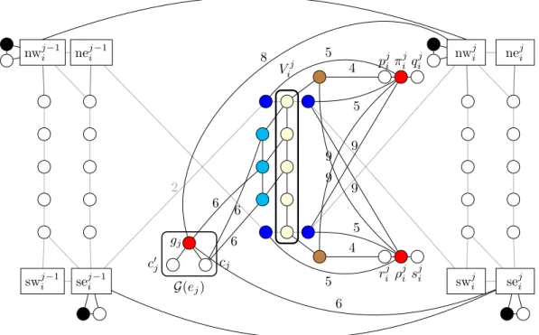
ofVij. For anyi∈[k] andj∈[m], we add toG0 two pairs of vertices{pji, qij}and {rji, sji}, and twogatesπji andρji. Vertexπji is adjacent topji andqji, and vertexρji is adjacent torji andsji.
We link vi,j1 topji, and vji,t to rij, each by a path of length t. It introduces two new neighbors ofvi,j1 andvi,tj (the brown vertices in Figure 4). We denote them by tbji and bbji, respectively. The blue and brown vertices are linked toπij andρji in the following way. We link tlji and trji toπijby a private path of lengtht, and toρji by a private path of length 2t−1. We link blji and brji to πij by a private path of length 2t−1, and toρji by a private path of lengtht. (Let us clarify that the names of the blue vertices blji and brji are for “bottom-left” and “bottom-right”, andnot for “blue” and “brown”.) We link tbji (neighbor ofvji,1) toρji by a private path of length 2t−1. We link bbji (neighbor ofvi,tj ) toπij by a private path of length 2t−1. Note that the general rule to set the path length is to match the distance between the neighbor inVij andpji (resp.rji). With that in mind we link, if it exists, the top cyan vertex tcji (the one with smallest indexγ) neighboringVij to πij with a path of length dist(vi,γj , pji) =t+γ−1 wherevji,γ is the unique vertex inN(tcji)∩Vij. Observe that with the notations of the previous section tcji =eji,γ. We also link, if it exists, the bottom cyan vertex bcji (the one with largest indexγ) toρji with a path of length dist(v, rij) wherev is again the unique neighbor of bcji in Vij.
It can be observed that we only have two paths (and not all six) from the at most three cyan vertices to the gatesπji andρji. This is where the edges between the cyan vertices will become relevant. See Figure 4 for an illustration of the forced vertex gadget, keeping in mind that, for the sake of legibility, four paths to{πij, ρji}are not represented.
5.1.2
Forced vertex gadget
We now deal with the issue (2). Bywe add (orattach)a forced vertex to an already present vertexv, we mean that we add two adjacent neighbors to v, and that these two vertices remain of degree 2 in the whole graphG00. Hence one of the two neighbors will have to be selected in the resolving set since they are true twins. We callforced vertex one of these two vertices (picking arbitrarily).
For everyi∈[k] andj ∈[m], we add a forced vertex to the gates nwji and seji ofPij,j+1. We also add a forced vertex to each vertex in N({πij, ρji})\ {pji, qij, rji, sji}. This represents a total of 12 vertices (6 neighbors ofπij and 6 neighbors ofρji). For everyj ∈[m], we attach a forced vertex to each vertex inN(gj)\ {cj, c0j}. This constitutes 14 neighbors (hence 14 new
forced vertices). Therefore we setk00:=km+ 12km+ 2km+ 14m= 15km+ 14m.
5.1.3
Finishing touches and useful notations
We use the convention that P(u, v) denotes the path fromu tov which was specifically built fromutov. In other words, forP(u, v) to make sense, there should be a point in the construction where we say that we add a (private) path betweenuandv. For the sake of legibility,P(u, v) may denote either the set of vertices or the induced subgraph. We also denote byν(u, v) the neighbor ofuin the path P(u, v). Observe thatP(u, v) is a symmetric notation but notν(u, v).
We add a path of length dist(ν(πji,trji),swji) =t betweenν(πij,trji) and seji, and a path of length dist(ν(πji,blij),neji−1) = 2t−1 betweenν(πji,blji) and nwji−1. Similarly, we add a path of length dist(ν(ρji,trji),swji) = 2t−1 betweenν(ρji,trji) and seji, and a path of length dist(ν(ρji,blji),neji−1) =t betweenν(ρji,blji) and nwji−1. We added these four paths so that no forced vertex resolves any critical pair in the propagation gadgetsPij−1,j andPij,j+1.
Vij G(ej) gj cj c0j 6 6 6 swji seji nwji neji swji−1 seji−1 nwji−1 neji−1 2 4 4 p j i π j i q j i rij ρji sji 5 9 5 9 5 5 8 6 9 9
Figure 4 Vertices tlji,trji,blji,brji (blue vertices) are linked toπij,ρji by paths of appropriate lengths (see Section 5.1.1). Vertex tbji is linked by a path toρji, while bbji is linked by a path toπij. To avoid cluttering the figure, we did not represent four paths: from tlji and bc
j i toρ
j
i, and from blji and tcji toπji. We also did not represent the paths already in thek-MRS-instance from the blue vertices togj. Black vertices are forced vertices. Gray edges are the edges in the propagation gadgets already depicted in Figure 3. Not represented on the figure, we add a forced vertex to each neighbor of the red vertices, exceptpji, qij, rij, sji, cj, c0j. Finally we add four more paths and potentially two edges (see Section 5.1.3).
Finally we add an edge betweenν(gj,nw j
i) andν(cj,bc j
i) wheneverV j
i have exactly three
cyan vertices. We do that to resolve the pair {ν(cj,tcji), ν(cj,bcji)}, and more generally
every pair{x, y} ∈P(cj,tc j
i)×P(cj,bc j
i) such that dist(cj, x) = dist(cj, y). This finishes
the construction of the instance (G00, k00:= 15km+ 14m) of Metric Dimension.
5.2
Correctness of the reduction
The two next lemmas will be crucial in Section 5.2.1. The first lemma shows how the forcing set gadget simulates the action of former setX.
ILemma 6(?). For everyi∈[k]andj ∈[m], ∀v∈Vij,v resolves both pairs{pji, qij} and{rji, sji},
∀v /∈Vij,v resolves at most one pair of{pji, qij} and{rij, sji},
∀v /∈Vij∪P(vi,j1, pji)∪P(vi,tj , rji)∪ {qji, sji},v does not resolve{pji, qji} nor{rji, sji}. For Section 5.2.1, we also need the following lemma, which states that the forced vertices do not resolve critical pairs.
5.2.1
MD-instance has a solution
⇒
k-MRS-instance has a solution
Let S be a resolving set for the Metric Dimension-instance. We show that S0 :=S∩ Si∈[k],j∈[m]V
j
i is a solution fork-Multicolored Resolving Set. The setS\S0 is made of
14km+ 14mforced vertices, none of which is in someVij∪P(vi,j1, pji)∪ {qij} ∪P(vi,tj , rij)∪ {sji}. Thus by Lemma 6,S\S0 does not resolve any pair{pji, qij}or{rij, sji}. NowS0 is a set of k00−(14km+ 14m) =kmvertices resolving all the 2kmpairs{pij, qij}and{rji, sji}. Again by Lemma 6, this is only possible if|S0∩Vij|= 1. ThusS0 is a legal set of sizek0 =km. Let us now check thatS0 resolves every pair ofP in the graphG0.
By Lemma 7,S\S0 does not resolve any pair ofP in the graphG00. ThusS0 resolves all the pairs ofP inG00. Since the distances betweenVij and the critical pairs in the edge and propagation gadgetsVij is attached to are the same inG0 and inG00,S0 also resolves every pair ofP in G0. ThusS0 is a solution for thek-MRS-instance.
5.2.2
k-MRS-instance has a solution
⇒
MD-instance has a solution
Let S be a solution for k-Multicolored Resolving Set. We show that S0 := S∪F,whereF is the set of forced vertices, is a solution forMetric Dimension.
ILemma 8(?). Every vertex inG00 is distinguished byS0.
The reduction is correct and it takes polynomial-time in |V(G)| to computeG00. The maximum degree ofG00 is 16. It is the degree of the verticesgj (nw
j i and se
j
i have degree at
most 11,πij andρji have degree 8, and the other vertices have degree at most 5). We use the pathwidth characterization of Kirousis and Papadimitriou [19], to show:
ILemma 9(?). pw(G00)690k+ 83.
Then solvingMetric Dimensionon constant-degree graphs in timef(pw)no(pw) could be used to solve k-Multicolored Independent Setin timef(k)no(k), disproving the ETH.
References
1 Florian Barbero, Lucas Isenmann, and Jocelyn Thiebaut. On the Distance Identifying Set Meta-Problem and Applications to the Complexity of Identifying Problems on Graphs. In
13th International Symposium on Parameterized and Exact Computation, IPEC 2018, August
20-24, 2018, Helsinki, Finland, pages 10:1–10:14, 2018. doi:10.4230/LIPIcs.IPEC.2018.10.
2 Zuzana Beerliova, Felix Eberhard, Thomas Erlebach, Alexander Hall, Michael Hoffmann, Matús Mihalák, and L. Shankar Ram. Network Discovery and Verification. IEEE Journal on
Selected Areas in Communications, 24(12):2168–2181, 2006. doi:10.1109/JSAC.2006.884015.
3 Rémy Belmonte, Fedor V. Fomin, Petr A. Golovach, and M. S. Ramanujan. Metric Dimension of Bounded Tree-length Graphs. SIAM J. Discrete Math., 31(2):1217–1243, 2017. doi: 10.1137/16M1057383.
4 Gary Chartrand, Linda Eroh, Mark A. Johnson, and Ortrud Oellermann. Resolvability in graphs and the metric dimension of a graph. Discrete Applied Mathematics, 105(1-3):99–113, 2000. doi:10.1016/S0166-218X(00)00198-0.
5 Marek Cygan, Fedor V. Fomin, Lukasz Kowalik, Daniel Lokshtanov, Dániel Marx, Marcin Pilipczuk, Michal Pilipczuk, and Saket Saurabh. Parameterized Algorithms. Springer, 2015. doi:10.1007/978-3-319-21275-3.
6 Josep Díaz, Olli Pottonen, Maria J. Serna, and Erik Jan van Leeuwen. Complexity of metric dimension on planar graphs. J. Comput. Syst. Sci., 83(1):132–158, 2017. doi:10.1016/j. jcss.2016.06.006.
7 Rodney G. Downey and Michael R. Fellows. Fundamentals of Parameterized Complexity. Texts in Computer Science. Springer, 2013. doi:10.1007/978-1-4471-5559-1.
8 David Eppstein. Metric Dimension Parameterized by Max Leaf Number. J. Graph Algorithms
Appl., 19(1):313–323, 2015. doi:10.7155/jgaa.00360.
9 Leah Epstein, Asaf Levin, and Gerhard J. Woeginger. The (Weighted) Metric Dimension of Graphs: Hard and Easy Cases. Algorithmica, 72(4):1130–1171, 2015. doi:10.1007/ s00453-014-9896-2.
10 Henning Fernau, Pinar Heggernes, Pim van ’t Hof, Daniel Meister, and Reza Saei. Computing the metric dimension for chain graphs. Inf. Process. Lett., 115(9):671–676, 2015. doi: 10.1016/j.ipl.2015.04.006.
11 Florent Foucaud, George B. Mertzios, Reza Naserasr, Aline Parreau, and Petru Valicov. Identification, Location-Domination and Metric Dimension on Interval and Permutation Graphs. II. Algorithms and Complexity. Algorithmica, 78(3):914–944, 2017. doi:10.1007/ s00453-016-0184-1.
12 Michael R. Garey and David S. Johnson.Computers and Intractability: A Guide to the Theory
of NP-Completeness. W. H. Freeman, 1979.
13 Frank Harary and Robert A Melter. On the metric dimension of a graph. Ars Combin, 2(191-195):1, 1976.
14 Sepp Hartung and André Nichterlein. On the Parameterized and Approximation Hardness of Metric Dimension. InProceedings of the 28th Conference on Computational Complexity, CCC
2013, K.lo Alto, California, USA, 5-7 June, 2013, pages 266–276, 2013. doi:10.1109/CCC.
2013.36.
15 Stefan Hoffmann, Alina Elterman, and Egon Wanke. A linear time algorithm for metric dimension of cactus block graphs. Theor. Comput. Sci., 630:43–62, 2016. doi:10.1016/j.tcs. 2016.03.024.
16 Stefan Hoffmann and Egon Wanke. Metric Dimension for Gabriel Unit Disk Graphs Is NP-Complete. InAlgorithms for Sensor Systems, 8th International Symposium on Algorithms for Sensor Systems, Wireless Ad Hoc Networks and Autonomous Mobile Entities, ALGOSENSORS
2012, Ljubljana, Slovenia, September 13-14, 2012. Revised Selected Papers, pages 90–92, 2012.
doi:10.1007/978-3-642-36092-3_10.
17 Russell Impagliazzo, Ramamohan Paturi, and Francis Zane. Which Problems Have Strongly Exponential Complexity? Journal of Computer and System Sciences, 63(4):512–530, December 2001.
18 Samir Khuller, Balaji Raghavachari, and Azriel Rosenfeld. Landmarks in Graphs. Discrete
Applied Mathematics, 70(3):217–229, 1996. doi:10.1016/0166-218X(95)00106-2.
19 Lefteris M. Kirousis and Christos H. Papadimitriou. Interval graphs and searching. Discrete
Mathematics, 55(2):181–184, 1985. doi:10.1016/0012-365X(85)90046-9.
20 Daniel Lokshtanov, Dániel Marx, and Saket Saurabh. Lower bounds based on the Exponential Time Hypothesis. Bulletin of the EATCS, 105:41–72, 2011. URL:http://eatcs.org/beatcs/ index.php/beatcs/article/view/92.
21 Krzysztof Pietrzak. On the parameterized complexity of the fixed alphabet shortest common supersequence and longest common subsequence problems. J. Comput. Syst. Sci., 67(4):757– 771, 2003. doi:10.1016/S0022-0000(03)00078-3.
Table 1Glossary of the construction.
Symbol/term Definition/action
{aji,γ, αji,γ} critical pair of the propagation gadgetPij,j+1
Aji set of vertices S γ∈[t]{a j i,γ, α j i,γ}
bbji bottom brown vertex, ν(vi,tj , rji)
bcji bottom cyan vertex (smallest indexγ)
blji neighbor ofvi,tj in Pij−1,j
blue vertex one of the four neighbors ofVij in the propagation gadgets
brji neighbor ofvji,t inPij,j+1
brown vertex verticesν(vji,1, pij) andν(vji,t, rij) {cj, c0j} critical pair of the edge gadgetG(ej)
cyan vertex neighbor ofVij in the paths toG(ej)
Eij vertices in the paths fromVij to G(ej)
eji,γ alternative labeling of the cyan vertices, neighbor of vji,γ
F set of all forced vertices
G(ej) edge gadget on{gj, cj, c0j}betweenV j
i andV
j
i0, where ej∈E(Vi, Vi0)
mcji middle cyan vertex (not top nor bottom)
neji north-east gate ofPij,j+1
nwji north-west gate ofPij,j+1
neji, swji resolve the critical pairs of Pij,j+1 nwji, seji do not resolve the critical pairs ofPij,j+1
ν(u, v) neighbor ofuin the pathP(u, v)
P list of critical pairs
{pji, qij} pair only resolved by vertices inVij∪P(vji,1, pji)∪ {qij} πji gate of{pji, qij}, linked by paths to most neighbors ofVij Pij,j+1 propagation gadget betweenVij andVij+1
P(u, v) path added in the construction expressly betweenuand v {rji, sji} pair only resolved by vertices inVij∪P(vji,t, rij)∪ {sji}
ρji gate of {rji, sji}, linked by paths to most neighbors ofVij
seji south-east gate ofPij,j+1
swji south-west gate ofPij,j+1
t size of eachVi
tbji top brown vertex,ν(vi,j1, pji)
tcji top cyan vertex (largest indexγ)
tlji neighbor ofvji,1 in Pij−1,j
trji neighbor ofvi,j1in Pij,j+1
Vi partite set ofG
Vij “copy ofVi”, stringed by a path, in G0 andG00
vji,γ vertex ofVij representingvi,γ ∈V(G)
Wj endpoints inVij∪V j i0 of paths fromV j i ∪V j i0 toG(ej)
X set containing all the setsVij fori∈[k] andj∈[m] Xj neighbors ofWj on the paths toG(ej) (cyan vertices)