Planning & Acting: Optimal Markov Decision
Scheduling of Aggregated Data in WSNs by
Genetic Algorithm
Imane Horiya Brahmi
∓, Florian Maire
‡, Soufiene Djahel
∓and John Murphy
∓ ∓ Lero, UCD School of Computer Science and Informatics, Ireland‡ UCD, School of Mathematical Sciences, Insight Centre for Data Analytics, Ireland {horiya-imane.brahmi, florian.maire, soufiene.djahel, j.murphy}@ucd.ie
Abstract—Data aggregation techniques have emerged as promising solutions for extending Wireless Sensor Networks (WSNs) lifetime. However, this approach suffers from a design issue in delivering the strict requirements needed by some monitoring applications. Carefully balancing Energy, Delay and Accuracy is essential for achieving these requirements. In this work, we focus on distributed data aggregation, where a sensor estimates the network information by the exchange of readings with different priority levels. We then propose an optimal decision policy for scheduling the transmission of the aggregated data at the node level. To model the investigated problem, we first adopt Markov Decision Process (MDP) whereby we define the reward function. Then, we apply a Genetic Algorithm (GA) to find a set of optimal decisions that ensures the best trade-off between energy saving, delay and accuracy of the received data based on their priority level. The simulation results yield excellent performance and our optimization shows a significant enhancement up to 20% compared to the other policies.
Keywords – WSNs, Data aggregation, Delay-Energy-Accuracy tradeoff, Markov Decision Process (MDP), Genetic Algorithm (GA)
I. INTRODUCTION
WSNs [1] have attracted significant attention in recent years for their potential to replace many of the existing wired sensing technologies, as well as providing new platform solution where wired solutions are hard to deploy and maintain.
Although WSNs technology offers low cost and flexible solution for several monitoring applications, the high dependency of sensors on limited energy sources impedes its wide deployment. One basic approach to alleviate the consequences for this problem is to use in-network data aggregation and processing. This solution filters the received readings from different sources; combines them into one packet, thereby reducing the number of the transmitted packets and thus, the overall energy consumption in the network.
The critical challenge in designing the aggregation approach in WSNs is meeting the requirements imposed by various monitoring applications. Those requirements consist mainly in optimizing the delay incurred by the waiting time before transmitting the resulting packet from aggregation, as well as energy consumption in the node while insuring the highest accuracy of the transmitted data. For instance time-sensitive applications such as disaster relief, etc. require a short waiting times before forwarding the aggregated data. In contrast, periodic monitoring applications (with lower priority) are more sensitive to the accuracy of data being collected in terms of the achieved level of representativeness. An omnipresent requirement to both types of applications is energy saving for increasing the network lifetime.
We consider a scenario of distributed data aggregation, where each sensor can estimate the state of the network by exchanging its local
readings with the neighbors [2]. The aggregated information is then made available to the end user at anytime in any node. In this context, each node should carefully decide whether to stop the aggregation process and transmit/forward the resulting packet, at a given medium access opportunity, or wait till the next access opportunity in order to increase the achieved reward. Moreover, in the scenarios where sensor nodes detect/forward various types of parameters with different priority levels, decisions should be taken according to the content of these different types of the message in order to fulfill the application constraints.
In this paper, we address the problem of optimal stopping at the node level, based on the received information, by:
(i) embedding the decision problem in a Markov Decision Process (MDP) [3] framework,
(ii) determining the optimal policy for the node to schedule the transmission of their aggregated packet using a Genetic Algo-rithm (GA) [4].
Therefore, at each access to the medium, this scheme allows the sensors to predict the future states of the network in order to act according to the best decision (to send or to postpone the aggregated packet). By construction of our model, a tradeoff between the energy consumption, the delay (i.e. waiting time) and the accuracy (i.e. the level of representativeness) is fulfilled.
The remainder of the paper is organized as follows: in Section II we briefly review some related works. Section III gives a detailed overview of our model and solve our optimization problem. In Section V, we assess our proposal and present/discuss the obtained simulation results. Finally, we conclude in Section VI.
II. RELATED WORK
MDPs framework has been widely used in uncertain environment and dynamic systems in order to optimize the network resources in WSNs. The authors of [5] reviewed in a survey different works on MDP and its applications in WSNs. In their paper the authors have discussed some MDP designs concerning data exchange and topology formation [6], resource and power optimization [7], security challenges [8], etc.
Related ideas in the literature have used this framework for different purposes, either for ensuring the tradeoff between energy saving and transmission delay or energy, throughput and delay. For example in [2] the authors study the fundamental trade-off between energy saving and transmission delay of the packets in distributed data aggregation. The main objective was to maximize a reward function involving an aggregation gain and a discount due to the waiting time. The authors proposed two learning-based distributed approximation algorithms that perform close to the optimal solution. In this work the representativeness of the received data is not considered in the decision-making. The authors of [9] used MDP in order to select messages forwarding based on the importance
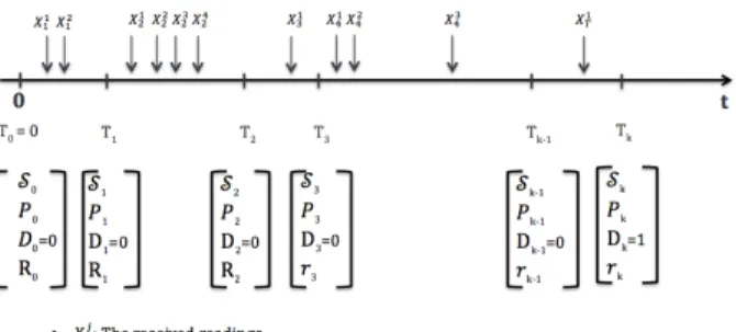
Figure 1: An illustration of the decision process
of the message and the energy level of the nodes. In this work the authors consider the scenario where sensors act as a relay of different priority packets. The authors used the MDP in order to determine which packets need to be sent and which one will be discarded based on the priority level of the messages. In [10] an application-oriented dynamic tuning methodology for WSNs based on MDP was proposed. The main objective in this work is to optimize a reward function that combine power consumption, throughput and delay. All the above related methodologies, involve the so-called Bellman equations which are, most of the time, intractable. As a result, they resort to numerical approximations which represent a computational burden. In addition, designing an aggregation scheme considering different types of packets and ensuring a tradeoff between energy delay and accuracy was not addressed in previous works. Our approach addresses this in the next subsections.
III. PROBLEMFORMULATION
We consider the scenario of structure-free distributed data aggre-gation in WSNs. Sensor nodes can estimate the information of the whole network through data exchange and aggregation with their neighboring nodes. We assume that we have no sink and the estimated information on the state of the network is available at any sensor node in the network, at any time. The exchange of the information is asynchronous and the arrival of samples at any node is random. The arrival of samples at each node can be either from its local sensing activities or neighboring nodes. The aggregation process starts at each sensor node upon reception of the first arrival sample. Once the channel is sensed as free, the aggregated packet can be sent. It is worth to mention that, in this work, a random channel access scheme is assumed due to the popularity of such scheme in WSNs [11].
The objective of the paper is to determine an optimal decision policy that achieves Energy-Delay-Accuracy tradeoff at each node.
We define Tk as the time period from when a node gets the
first sample to the kth availability of the multiaccess channel for
transmission as shown in the Figure 1. Let us denote
• {Tk, k >0} the sequence of random variables corresponding
to the times where the node has access to the medium
• {Nk, k > 0}the number of received readings from the time
T0 to thek-th access to the medium,Tk
• Xij the random variable which represents the j-th received
reading by the node during the interval(Ti−1, Ti)
At each access to the medium a node evaluate its state. Att=Tk
we have the following observations:
• (X11, .., X N1 1 )between(T0, T1) • (X21, .., X N2−N1 2 )between(T1, T2) .. . • (Xk1, .., XkNk−Nk−1)between(Tk−1, Tk)
Each node evaluates the received readings and decides whether it should stop waiting for more readings, allowing to save energy and
to reduce the delays, or if it should postpone the decision until the next interval to receive more readings, hence improving the accuracy. We formulate the decision problem with a Markov Decision Process (MDP) model characterized by the following tuple (S, D, P, R), where:
• S is the set of states
• D={0,1}is the set of possible decisions
• P is a transition probability, it’s the measure of the next state
given the current state and the current decision
• Ris the reward function A. States of the node
At each available access to the mediumTk, a node evaluates its
state Sk. This is modeled as a vector containing all the available
information to make decision at time Tk and is defined by the
following four parameters:
Sk= (Ek, Wk, Xk, Ak), (1)
where:
• Ek: Energy level at timeTk
• Wk: Delay, defined as the waiting time since the last
transmis-sion
• Xk= (Xk1, .., X
Nk−Nk−1
k ): Set of all the received observations
fromTk−1 toTk with their priority level
• Ak: Accuracy at timeTk
Following [9], Ek is defined as the available energy at time Tk
and depends on the decisionDk−1
Ek=Ek−1−Dk−1C1,k−1−(1−Dk−1)C0,k−1, (2)
where C1,k−1 is the energy consumed when the node decides to
stop the aggregation and transmit the resulting packet, andC0,k is
the energy consumed for staying alive untilTk(i.e. sensing/receiving
information while waiting for more packets).
The second parameter of the node state is the waiting timeWk. At
timeTk, denoting byTk(last) the time of last transmission, we have:
Wk=Tk−Tk(last)=Wk−1+Tk−Tk−1. (3)
We choose an exponential distribution to model the time between two consecutive medium access for a given node[2]. Therefore,
Tk−Tk−1is an exponential random variable with parameterδ >0.
Finally, conditionally on Wk−1 = wk−1, Wk is a shifted random
variable:
Wk=wk−1+τ , τ ∼exp(δ), (4)
For i ∈ {1,2, . . . , k}, Xi1, Xi2, . . . , X Ni−Ni−1
i is the set of
received readings by a node. We assume that the random variable
Nk, denoting the number of messages betweenTk−1andTkfollows
a Poisson distribution with parameterλi.e.
P(Nk−Nk−1=n|Tk−Tk−1=τ) =
(λτ)n
n! exp(−λτ), (5) The state of the node depends also on the accuracy of the received observations. We define the accuracy based on the representativeness of the received data. However, there are other parameters which can also be considered in defining the accuracy of the received observation such as: the instant of samples generation, number of samples or the value of the received observations. In this work, we focus on the representativeness of the data in a finite set of sensors and define it as follows:
Ak= Nk−Nk−1 N brtot if Dk−1= 1 Ak−1+ Nk−Nk−1 N brtot if Dk−1= 0 (6) where, N brtot is the total number of expected packets from the
B. Decision Epochs
At time Tk, the sensor node must take the decisionDk either to
send (Dk= 1) or to continue waiting (Dk= 0). The stopping policy
Π =
D1, D2, ..., Dk, ... represents a sequence of decision rules,
and depends on the state vector i.e.
Dk=dk(sk) =dk(Xk, Ek, Tk, Ak). (7)
Our ultimate goal is to find the set of decisions {D1, D2, ...} that
maximize an expected reward function (see Section III-D).
C. State Dynamics
Following the model introduced in the previous sections, we define the probability of any transition from state Sk−1 to Sk. Let
P(Sk|Sk−1, Dk−1) represent the probability of reaching a stateSk
knowing the stateSk−1 and the decisionDk−1:
P(Sk|Sk−1, Dk−1) =P(Xk, Ak, Wk, Ek|Sk−1, Dk−1). (8)
We assume that δ and λ are two known real positive constants. Since the parameters are non independent, we consider the following hierarchical model:
• Ek depends onEk−1,Dk−1 • Wk depends onWk−1,Dk−1
• Ak depends onAk−1,Dk−1,Wk,Wk−1 • Xk depends onAk,Ak−1,Dk−1
Using the total law of probability, this writes
P(Sk|Sk−1, Dk−1) =P(Xk|Dk−1, Sk−1, Ak, Wk, Ek)×
P(Ak|Ak−1, Dk−1, Sk−1)× P(Wk|Wk−1, Dk−1)×
P(Ek|Ek−1, Dk−1). (9)
First, let us provide the transition probability of the energy Ek
knowing Ek−1 and Dk−1. For any e > 0 and given Ek−1 and Dk−1, the probability ofEk=eis P(Ek = e|Ek−1, Dk−1) = ( P(Ek=e|Ek−1, Dk−1= 0) P(Ek=e|Ek−1, Dk−1= 1) (10) P(Ek=e|Ek−1, Dk−1= 0) = ( 1 if e=Ek−1−C0,k 0 otherwise (11) P(Ek=e|Ek−1, Dk−1= 1) = ( 1 if e=Ek−1−C1,k 0 otherwise (12) We now focus on the transition of the waiting time Wk, given
Wk−1 andDk−1. IfDk−1= 1, then the waiting time has been reset
at timeTk−1and a new receiving period has started. In this case, for
anywk>0, we have:
P(Wk=wk|Wk−1=wk−1, Dk−1= 1) =δexp(−δwk). (13)
Otherwise, ifDk−1= 0, the waiting time is incremented with a draw
from an exponential distribution with parameter δ:
P(Wk=wk|Wk−1=wk−1, Dk−1= 0)
=
δexp(−δ(w
k−wk−1)) if wk≥wk−1
0 otherwise (14)
In our data model, each readingXij is a random variable which
takes its values in{1,2}:
• Xki= 1refers to applications sensitive to the delay • Xki= 2refers to applications sensitive to the accuracy
We assume that they are independent from each other and that a priori, a message of class 1 (resp. of class 2) is received with probabilityρ(resp. with probability1−ρ). This yields:
P n Xk= Xk(1), Xk(2), ..., X(Nk−Nk−1) k |Nk, NK−1 o = ρ PNk i=11{Xik=1}× (1−ρ) PNk i=11{Xik=2} . (15) Using the law of total probability, we provide the transition for the accuracyAk: P(Ak=a|Ak−1, Wk, Wk−1, Dk−1) = P∞ n=0Pr(Ak=a∩Nk=n|Ak−1, Wk, Wk−1, Dk−1) = ∞ X n=0 Pr(Ak=a|Nk=n, Ak−1, Wk, Wk−1, Dk−1)× Pr(Nk=n|Wk, Wk−1, Dk−1) = ∞ X n=0 1(A k−1+Nk −Nk−1 N brtot ) ×(λτ) n n! exp(−λτ) D. Reward Function
The reward function is a deterministic function and depends on the energy consumption of the node, the delay (waiting time) and the accuracy of the received packets:
Rk=F(Ek, Wk, Ak). (16)
This reward function Rk(Sk, Dk) is determined at each access
opportunity to the medium, given the node stateSkand the decision
takenDk. We define it as follows:
Rk(Sk, Dk) =ωEFE(Sk, Dk) +ωWFW(Sk, Dk)+
ωAFA(Sk, Dk), (17)
whereFE(Sk, Dk),FW(Sk, Dk),FA(Sk, Dk)represent the energy,
delay and accuracy reward functions respectively, andωE,ωW and
ωAare their corresponding weight factors.
The energy and the accuracy reward functions are defined in the equation (2) and (6). Therefore, we define the delay function as cited in [10]: FW(Sk, Dk) = 1, 0< Wk≤LD (UD−Wk) (UD−LD), LD< Wk< UD 0, Wk≥UD (18)
whereWkis the waiting at timeTkandLDandUDare two constants
defining the lower and upper tolerated delay respectively. These two delays can be set based on the application requirement.
We assumed in our work that the sensors in the network collect two different types of data with different priority levels. Therefore, we define two different sets of weightsωrI forI∈ {E, W, A}where
r∈ {1,2}.ωrIdepends on the message type, so that the delay reward
function will have a higher weight value when Xki = 1 and the
accuracy reward function will have a higher weight value whenXki =
2. We keep the same weight for the energy reward function for both messages. Finally, we weight our function according to the number of the received messages for each category, as it is shown in the following equation: Rk(Sk, Dk) = 2 X r=1 #{Xi k=r} N brk × ωErFE(Sk, Dk) +ωrW FW(Sk, Dk) +ωArFA(Sk, Dk) , (19)
E. Optimality Equation
For a given stateSk, a sensor node makes a decisionDk∈ {0,1}.
The set of all decision is called the policy π ∈ {0,1}∞
. There-fore, the reward received by the node at time k is Rk(Sk, Dk).
The expected total reward vk over the decisions making horizon
πk= (Dk, . . . , D∞)is equal to: vk(πk) =Rk(Sk, Dk) +E ( ∞ X t=k+1 Rt(St, Dt) πk ) | {z } ψ(πk,Sk) . (20)
We assume a finite decision making horizon H for the expected total reward vk(πk), such that:
ψ(πk, Sk) = Z · · · Z H X t=k+1 Rt(St, Dt) f(St+1, St+2, ..., SH)|Sk, πk)dSt+1. . .dSH, (21)
wheref denotes the probability density function of the future states
St+1, . . . , SH given the current state Sk and the decision making
horizonπk= (Dk, Dk+1, . . . , DH).
Our objective is to find the policy πk ∈ {0,1}H−k+1, that
maximizesvk(πk)
πk∗= arg max πk∈{0,1}H−k+1
vk(πk), (22)
The total expected reward involves the actual rewardRk(Sk, Dk),
defined in (19) and the expected rewardψ(πk, Sk). However, because
of the underlying MDP model, an analytical expression ofψ is not available. We resort to a pointwise Monte-Carlo estimation of ψ
to overcome this issue and for a given (πk, Sk), we approximate
ψ(πk, Sk)by ˆ ψ(πk, Sk)≈ 1 Nsc Nsc X j=1 ( H X t=k+1 Rt(Stj, Dt) ) , (23)
where Nsc defines the number of scenarios in the Monte-Carlo
estimation. This number is set in the simulation part.
IV. SOLVING THEOPTIMALITYEQUATION USING AGA In this section, we solve our optimality equation and find a set of a finite optimal policyπˆt∗that optimizes the
ˆ
vk(πk) =Rk(Sk, Dk) + ˆψ(πk, Sk). (24)
We propose to use a Genetic Algorithm (GA) [4] in order to perform this optimization problem. The GA provides a smart meta-heuristic for solving combinational optimization problems [12] and is well suited to discrete optimization problems, that we are aiming to solve in (22). By analogy to evolutionary theories which predict that in a random population only the most adapted individuals to the environment will survive, the GA looks for the features that correspond to the fittest individual.
The GA starts by selecting successive generations from an initial random population, which corresponds to the a set of decisions in our context. At convergence, the GA will provide the fittest combinations from the last generation with respect to the environment (i.e. the best combination of decisions which maximize the reward function (19) after many generations). The Algorithm 1 summarizes the different steps performed at each iteration of the GA.
Algorithm 1
Input:A fitness functionvk(πk), the population sizeP opSize
and the number of generationsGenN br
(1) Initialisation: start with a random set of population
{πm1 }P opSizem=1 ,{πm1 } ∈ {0,1}H−k+1
(2) Evaluation:measure the fitness of the population by
com-putingvk(π1m)and keep the P opSizefittest individuals
(3) Selection:selectP opSize fittest couples
(4) Reproduction: each couple provides an individual, the
shared parent decisions are preserved while the remaining decisions are selected randomly.
Go to step (2) unless GenN br generations have been com-pleted.
V. PERFORMANCEEVALUATION
In this section we analyze the performance of our proposed scheme in different scenarios through simulations using Matlab and show the substantial gain achieved through the optimization scheme we propose. We first start by describing some common features of the experimental setup, followed up by the description of the obtained results.
• The random number of sample arrivals is assumed to have a Poisson distribution withλ= 10for the generation of readings during two consecutive access opportunities to the medium. The readings have different priority levels: we generate them with different probability ρ = 0.3 for Xi
k = 1 and 1−ρ
for Xi
k = 2. The weight is set to ω1 = [0.4,0.5,0.1] and
ω2 = [0.4,0.2,0.4]. This allows to privilege the delay when Xi
k= 1and the accuracy whenXki = 2. We have set the total
number of the neighbor each node toNtot= 20.
• We use an exponential model withδ= 6for the random
inter-arrival time of decision epochs (i.e. access to the medium). We use a simulation horizon of3time units.
• We have used a simple deterministic energy model fixed three
constant and known parameters: for allk >0, the energy spent on idle state C0,k = .01, the energy spent on transmitting a
single messageC1,k=.1andEinit= 1the initial energy.
• For the delay function, we have set the upper toUD = 1and
the lower delays toLD= 0.1.
• In our estimation, we have set the number of Monte Carlo simulations toNsc= 100.
• We have solved the optimization problem throughout the GA available in the Matlab Global Optimization Toolbox. We set the population size P opSize = 50and a generation number
GenN br= 5.
A. Results:
We have considered four schemes of policy design for the decision problem in distributed data aggregation: (1) our policy scheme using GA (Optimal Decision), (2) random decision (Random Decision), (3) decision policy which privileges delay transmission (i.e. the node send the resulting packet every time it gets access to the medium,
πW aitingT ime) and (4) decision policy which privileges the accuracy
of the data (i.e. the node send the resulting packet only when it receives all the expected packets,πAccuracy).
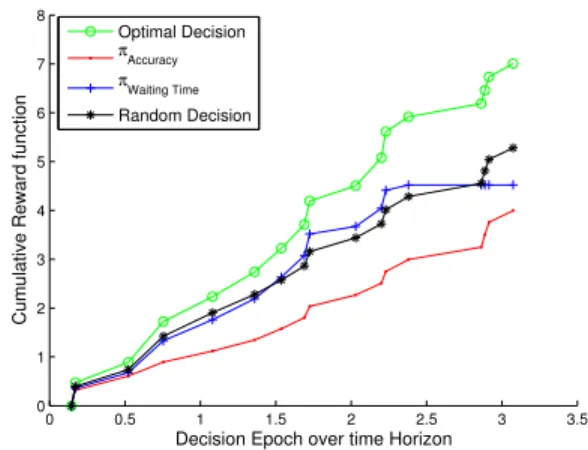
First, we show the impact of the different policy decisions on the reward function over the decision epochs for a finite horizonH. Figure 2 shows the gain achieved by our optimization compared to the three other schemes. We notice the general decreasing trend of the reward function over time. This is explained (i) since the energy
0 0.5 1 1.5 2 2.5 3 3.5 0 0.1 0.2 0.3 0.4 0.5 0.6 0.7 0.8 0.9
Decision Epoch over time Horizon
Reward function Optimal Decision π Accuracy π Waiting Time Random Decision
Figure 2: The impact of the different policy decisions on the Reward Function over the decision epoch
decreases every time a sensor node receives, waits or transmits data, (ii) because the delay penalizes the reward when it exceeds the upper bound. On the other side, the accuracy is likely to increase the reward function since more and more readings are available as time goes. The crucial feature of our solution is that it allows a tradeoff between the expected gain in accuracy and the expected losses due to the energy and the delay. In Figure 3, we show the impact of the cumulative reward function over time horizon: this allows to assess the significant gain offered by our scheme at a global scale.
We have used different finite decision horizons H ∈ {0,1,3} with Nsc = 100 in the Figure 4. The case H = 0 corresponds
to a maximization of the soleRk in (24) . As expected, the larger
the horizonH, the better the prediction and the greater the reward. Meanwhile, a large horizon H generates an heavy computational burden: indeed, the Monte-Carlo simulation forecasts the network state for a time window of lengthH. As shown in Figure 4, the benefit provided by increasingHis decreasing over time (the precision of the network state prediction indeed shrinks for distant states). This yields a tradeoff between the reward gain and the computational burden. In the present simulation,H= 1 provides a satisfactory tradeoff.
We show in Figure 5 how the different decisions influence the energy function for both type of messages since they have the same ω. The energy function decreases when the sensor nodes transmits at any medium access: this represents the worst case (see
πW aitingT ime). On the other hand, more energy is saved when there
is less transmission (πAccuracy). We notice from this figure that the
energy function observed with the optimal decision is close the best solution (πAccuracy). However, the decrease of all energy functions
is due to the packets send and received.
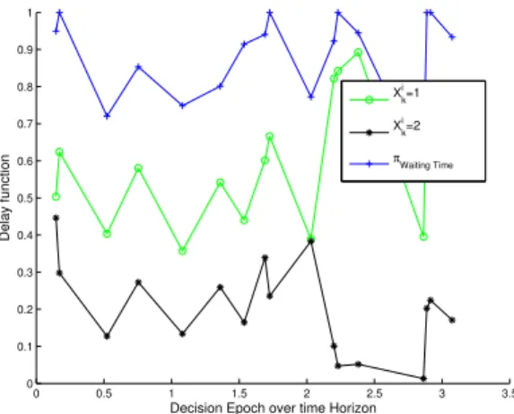
The last set of results in Figures 6 and 7 present the delay and accuracy functions for the different types of message. In this set of results, we compare our scheme with the best schemes:πW aitingT ime
for the delays plots andπAccuracy for the accuracy plots. This shows
how our results are close to these schemes, and how our scheme gives priority to the accuracy when the readings are more sensitive to the accuracy, and to the delay when they are sensitive to the waiting time.
In Figure 6, we show how the reading sensitive to the delay (Xi k=
1) achieves a lower delay function. Those results are quite similar to those achieved in the scenario where the sensors forward the resulted packet every time they have access to the medium πW aitingT ime.
Recall that when the waiting time is small, the delay function is equal to 1 (see equation (18)).
We show in Figure 7 how the accuracy function of the messages sensitive to the accuracy is almost equal to πAccuracy.
0 0.5 1 1.5 2 2.5 3 3.5 0 1 2 3 4 5 6 7 8
Decision Epoch over time Horizon
Cumulative Reward function
Optimal Decision π Accuracy π Waiting Time Random Decision
Figure 3: Cumulative Reward Function over time
0 0.5 1 1.5 2 2.5 3 3.5 0 1 2 3 4 5 6 7 8
Decision Epoch over time Horizon
Cumulative Reward function
Optimal Decision H=3 "Optimal Decision" H=0 Optimal Decision H=1
Figure 4: The impact of different finite decision horizons H
on the Cumulative Reward Function over time
0 2 4 6 8 10 12 14 16 18 0 0.1 0.2 0.3 0.4 0.5 0.6 0.7 0.8 0.9 1 Decision Epoch Energy function Optimal Decision Random Decision π Accuracy π Waiting Time
Figure 5: The impact of the different policy decisions on the Energy Function
0 0.5 1 1.5 2 2.5 3 3.5 0 0.1 0.2 0.3 0.4 0.5 0.6 0.7 0.8 0.9 1
Decision Epoch over time Horizon
Delay function
Xki=1
Xki=2
π
Waiting Time
Figure 6: The impact of the different policy decisions on the Delay Function 0 0.5 1 1.5 2 2.5 3 3.5 0 0.02 0.04 0.06 0.08 0.1 0.12 0.14 0.16 0.18
Decision Epoch over time Horizon
Accuracy function Xki=1 Xk i =2 π Accuracy
Figure 7: The impact of the different policy decisions on the Accuracy Function
VI. CONCLUSION
A common requirement in WSNs technology is the demand to operate under device constraints (i.e. sensor lifetime, delay, etc). However, in the scenarios where the nodes forward messages with different priority levels, finding the best trade-off between the energy consumption, the transmission delay and the achieved accuracy is essential for meeting the application requirements. This paper has introduced a new stochastic decision framework to find an optimal policy that ensures Energy-Delay-Accuracy tradeoff in distributed data aggregation in WSNs for multipurpose applications. We first applied Markov Decision Process (MDP) framework for analyzing the decision problem and proposed to use a GA to determine the current and future optimal times for scheduling the aggregated data. This ensures a trade-off between the above three metrics. The performance evaluation results highlight the effectiveness and have shown that our algorithm achieves optimal performance in balancing energy, delay and accuracy.
VII. ACKNOWLEDGEMENT
This work was supported by the Telecommunications Graduate Initiative (TGI) which is funded by the Higher Education Author-ity under the Programme for Research in Third-Level Institutions
(PRTLI) Cycle 5 and co-funded under the European Regional De-velopment Fund (ERDF). It was also supported, in part, by Science Foundation Ireland grant 10/CE/I1855 to Lero - the Irish Software Engineering Research Centre (www.lero.ie)
REFERENCES
[1] I. F. Akyildiz, W. Su, Y. Sankarasubramaniam, and E. Cayirci, “Wireless sensor networks: a survey,”Computer networks, vol. 38, no. 4, pp. 393– 422, 2002.
[2] Z. Ye, A. A. Abouzeid, and J. Ai, “Optimal stochastic policies for distributed data aggregation in wireless sensor networks,”Networking, IEEE/ACM Transactions on, vol. 17, no. 5, pp. 1494–1507, 2009. [3] M. L. Puterman,Markov decision processes: discrete stochastic dynamic
programming. John Wiley & Sons, 2014.
[4] D. E. Goldberg and J. H. Holland, “Genetic algorithms and machine learning,”Machine learning, vol. 3, no. 2, pp. 95–99, 1988.
[5] M. A. Alsheikh, D. T. Hoang, D. Niyato, H.-P. Tan, and S. Lin, “Markov decision processes with applications in wireless sensor networks: A survey,”arXiv preprint arXiv:1501.00644, 2015.
[6] J. Hao, Z. Yao, K. Huang, B. Zhang, and C. Li, “An energy-efficient routing protocol with controllable expected delay in duty-cycled wireless sensor networks,” inCommunications (ICC), 2013 IEEE International Conference on. IEEE, 2013, pp. 6215–6219.
[7] Z. Lin and M. van der Schaar, “Autonomic and distributed joint routing and power control for delay-sensitive applications in multi-hop wireless networks,” Wireless Communications, IEEE Transactions on, vol. 10, no. 1, pp. 102–113, 2011.
[8] X. Li, Y. Zhu, and B. Li, “Optimal anti-jamming strategy in sensor net-works,” inCommunications (ICC), 2012 IEEE International Conference on. IEEE, 2012, pp. 178–182.
[9] R. Arroyo-Valles, A. G. Marques, and J. Cid-Sueiro, “Optimal selective forwarding for energy saving in wireless sensor networks,” Wireless Communications, IEEE Transactions on, vol. 10, no. 1, pp. 164–175, 2011.
[10] A. Munir and A. Gordon-Ross, “An mdp-based application oriented optimal policy for wireless sensor networks,” inProceedings of the 7th IEEE/ACM International Conference on Hardware/Software Codesign and System Synthesis, ser. CODES+ISSS ’09, 2009, pp. 183–192. [11] A. Bachir, M. Dohler, T. Watteyne, and K. K. Leung, “Mac essentials for
wireless sensor networks,”Communications Surveys & Tutorials, IEEE, vol. 12, no. 2, pp. 222–248, 2010.
[12] R. V. Kulkarni, A. Forster, and G. K. Venayagamoorthy, “Computational intelligence in wireless sensor networks: A survey,” Communications Surveys & Tutorials, IEEE, vol. 13, no. 1, pp. 68–96, 2011.