Importance sampling for jump processes and
applications to finance
Laetitia Badouraly Kassim, J´
erˆ
ome Lelong, Imane Loumrhari
To cite this version:
Laetitia Badouraly Kassim, J´erˆome Lelong, Imane Loumrhari. Importance sampling for jump processes and applications to finance. Journal of Computational Finance, Incisive media Ltd, 2016, 19 (2), pp.109-139. <hal-00842362>
HAL Id: hal-00842362
https://hal.archives-ouvertes.fr/hal-00842362
Submitted on 8 Jul 2013
HAL is a multi-disciplinary open access archive for the deposit and dissemination of sci-entific research documents, whether they are pub-lished or not. The documents may come from teaching and research institutions in France or abroad, or from public or private research centers.
L’archive ouverte pluridisciplinaire HAL, est destin´ee au d´epˆot et `a la diffusion de documents scientifiques de niveau recherche, publi´es ou non, ´emanant des ´etablissements d’enseignement et de recherche fran¸cais ou ´etrangers, des laboratoires publics ou priv´es.
Importance sampling for jump processes and applications to
finance
Laetitia Badouraly Kassim∗ Jérôme Lelong∗ Imane Loumrhari∗ July 8, 2013
Abstract
Adaptive importance sampling techniques are widely known for the Gaussian setting of Brownian driven diffusions. In this work, we want to extend them to jump processes. Our approach relies on a change of the jump intensity combined with the standard exponential tilting for the Brownian motion. The free parameters of our framework are optimized using sample average approximation techniques. We illustrate the efficiency of our method on the valuation of financial derivatives in several jump models.
Keywords: Importance sampling; sample average approximation; adaptive Monte Carlo methods.
1
Introduction
Lévy models have become quite popular in finance over the last decade. Vanilla options are easily and efficiently priced using the Fast Fourier Transform approach developed by Carr et al. (1999) but things become far more delicate for exotic options, for which Monte Carlo often reveals as the only possible approach from a numerical point of view. This becomes even more true when dealing with high dimensional products. In this work, we want to propose an adaptive Monte Carlo method based on importance sampling for computing the expectation of a function of a Lévy process. As explained by Kiessling and Tempone (2011), when resorting to Monte Carlo approaches, infinite activity Lévy processes are often approximated by finite activity processes, which can always be represented as the sum of a continuous diffusion (ie. driven by a Brownian motion) and a compound Poisson process. In this work, we will concentrate on such jump diffusions with a Brownian driven part and a jump part written as a compound Poisson process or possibly the sum of independent compound Poisson processes in the multidimensional case.
We consider a mixed Gaussian and Poisson framework in which we would like to settle an adaptive Monte Carlo method based on some importance sampling approach. Let G = (G1, . . . , Gd) be a standard normal random vector inRdandNµ= (N1µ1, . . . , N
µp
p ) a vector of
p independent Poisson random variables with parametersµ= (µ1, . . . , µp). We assume that
G and Nµare independent. We focus on the computation of
E=E[f(G, Nµ)] (1.1)
∗Univ. Grenoble Alpes, Laboratoire Jean Kuntzmann, BP 53, 38041 Grenoble Cédex 9, FRANCE, e-mail:
[email protected], [email protected], [email protected]. This project was supported by the Finance for Energy Market Research Centre, www.fime-lab.org.
wheref :Rd×Np −→R satisfiesE[|f(G, Nµ)|]<∞.
Lemma 1.1. For any measurable functionh:Rd×Np −→R either nonnegative or such that E[|h(G, Nµ)|]<∞, one has ∀θ∈Rd, λ∈R∗ +p, E[h(G, Nµ)] =E h(G+θ, Nλ) e−θ·G− |θ|2 2 p Y i=1 eλi−µi µ i λi Niλi (1.2)
where Nλ is a vector of p independent Poisson random variables with parameters λ =
(λ1, . . . , λp).
The proof of this lemma relies on elementary variable changes. Lemma 1.1 enables us to introduce some extra degrees of freedom in the computation of E. When the expectation
E is computed using a Monte Carlo method, the Central Limit Theorem advises to use the representation of f(G, Nµ) with the smallest possible variable which
is achieved by choosing the parameters (θ, λ) which minimize the variance of of
f(G + θ, Nλ) e−θ·G−|θ| 2 2 Qp i=1eλi−µi µ i λi Niλi
. This raises several questions which are investigated in the paper. Does the variance of f(G+θ, Nλ) e−θ·G−|θ|
2 2 Qp i=1eλi−µi µ i λi Niλi
admits a unique minimizer? If so, how can it be computed numerically and how to make the most of it in view of a further Monte Carlo computation?
These questions are quite natural in the context of Monte Carlo computations and have already been widely discussed in the pure Gaussian framework. The first applications to option pricing of some adaptive Monte Carlo methods based on importance sampling goes back to the papers of Arouna (Winter 2003/04, 2004). These papers were based on a change of mean for the Gaussian random normal vectors and the optimal parameter was searched for by using some stochastic approximation algorithm with random truncations. This approach was later further investigated by Lapeyre and Lelong (2011) who proposed a more general framework for settling adaptive Monte Carlo methods using stochastic approximation, which is know to be a little tricky to fine tune in practical applications. To circumvent the delicate behaviour of stochastic approximation, Jourdain and Lelong (2009) proposed to resort to sample average approximation instead, which basically relies on deterministic optimization techniques. An alternative to random truncations was studied by Lemaire and Pagès (2010) who managed to modify the initial problem in order ta apply the more standard Robbins Monro algorithm. Not only have they applied this to the Gaussian framework but they have considered a few examples of Levy processes relying on the Esscher transform to introduce a free parameter. The idea of using the Esscher transform was also extensively investigated by Kawai (2007, 2008a,b).
In this work, we want to understand how the jump intensity of a Lévy process can be modified to reduce the variance. First, we explain the parametric importance sampling transformation we use for the Gaussian and Poisson parts. Then, in Section 2, we prove that this transfor-mation leads to a convex optimization problem and we study the properties of the optimal parameter estimator. Then, in Section 3, we explain how to use this estimator in a Monte Carlo method. We prove that this approach satisfies an adaptive strong law of large numbers and a central limit theorem with optimal limiting variance. Finally, in Section 4, we apply our methodology to option pricing with jump processes.
Notations.
• We encode any elements of Rm as column vectors.
• Ifx∈Rm,x∗ is a row vector. We use the “∗” notation to denote the transpose operator for vectors and matrices.
• If x, y ∈ Rm, x·y denotes the scalar product of x and y and the associated norm is denoted by | · |.
• If x∈Rm, diagm(x) is the matrix with diagonal elements given by the vectorx and all extra diagonal elements equal to zero.
• The matrix Im denotes the identity matrix in dimensionm.
• If x ∈ Rm, we defined d0(x) = min1≤i≤m|xi|which is the distance between x and the set {y∈Rm : Qm
i=1yi= 0}.
• We say that a random vector Xwith values inRmhas Poisson distribution with param-eter µ ∈ Rm if the Xi are independent and have Poisson distribution with parameter
µi.
2
Computing the optimal importance sampling parameters
2.1 Properties of the variance
Thanks to Lemma 1.1, the expectation E can be written
E=E f(G+θ, Nλ) e−θ·G− |θ|2 2 p Y i=1 eλi−µi µ i λi Niλi , ∀θ∈Rd, λ∈R∗+p.
Note that for the particular choice of θ= 0 and λ=µ, we recover Equation (1.1).
The convergence rate of a Monte Carlo estimator of E based on this new representation is governed by the variance off(G+θ, Nλ) e−θ·G−|θ|
2 2 Qp i=1eλi−µi µ i λi Niλi
which can be written in the formv(θ, λ)− E2 where
v(θ, λ) =E " f(G, Nµ)2e−θ·G+|θ| 2 2 p Y i=1 eλi−µi µ i λi Niµi# . (2.1)
This expression of v is easily obtained by applying Lemma 1.1 to the function h(g, n) =
f(g+θ, n)2e−2θ·g−|θ|2Qp i=1e2(λi−µi) µ i λi 2ni
. Applying the change of measure backward after computing the variance enables us to write the variance in a form which does not involve the parameters θ and λin the arguments of the functionf. This remark is of prime importance as it is the basement of the following key result stating the strong convexity of v.
Proposition 2.1. Assume that
(A1) i. ∃(n1, . . . , np)∈N∗p, s.t.P(|f(G,(n1, . . . , np))|>0)>0
Then, the function v is infinitely continuously differentiable, strongly convex and moreover the gradient vectors are given by
∇θv(θ, λ) =E " (θ−G)f(G, Nµ)2e−θ·G+|θ| 2 2 p Y i=1 eλi−µi µ i λi Niµi# (2.2) ∇λv(θ, λ) =E " a(Nµ, λ)f(G, Nµ)2e−θ·G+|θ| 2 2 p Y i=1 eλi−µi µ i λi Niµi# (2.3)
where the vector a(Nµ, λ) =
1−N µ1 1 λ1 , . . . ,1− Npµp λp ∗
. The second derivatives are defined by
∇2θ,θv(θ, λ) =E " (Id+ (θ−G)(θ−G)∗)f(G, Nµ)2e−θ·G+ |θ|2 2 p Y i=1 eλi−µi µ i λi Niµi# (2.4) ∇2θ,λv(θ, λ) =E " (θ−G)a(Nµ, λ)∗f(G, Nµ)2e−θ·G+|θ| 2 2 p Y i=1 eλi−µi µ i λi Niµi# (2.5) ∇2λ,λv(θ, λ) =E " (D+a(Nµ, λ)a(Nµ, λ)∗)f(G, Nµ)2e−θ·G+|θ| 2 2 p Y i=1 eλi−µi µ i λi Niµi# (2.6)
where the diagonal matrix Dis defined by D= diagp
Nµ1 1 λ2 1 , . . . ,Npµp λ2 p .
Proof. Let us define the function F :Rd×Rd×R∗
+p −→Rby F(g, θ, n, λ) =f(g, n)2e−θ·g+|θ| 2 2 p Y i=1 eλi−µi µ i λi ni . (2.7)
For any values of (g, n), the function (θ, λ) 7−→F(g, θ, n, λ) is infinitely continuously differ-entiable. Since for all 0< m < M,
sup |(θ,λ)|≤M,m<d0(λ) |∂θjF(G, θ, N µ, λ)| ≤ M+ eGj+ e−Gjf(G, Nµ)2eM2/2+pM d Y k=1 (eM Gk+ e−M Gk) p Y i=1 e−µi µ i m Niµi (2.8)
where the right hand side is integrable because by Hölder’s inequality and Assumption (A1-ii), we have that for all (θ, λ)∈Rd×Rp,E(f(G, Nµ)2eθ·G+λ·Nµ)<∞. Hence, Lebesgue’s theorem ensures that v is continuously differentiable w.r.t. θand ∇θv is given by Equation (2.2).
We proceed similarly for the derivative w.r.t. λby using the following upper bound sup |(θ,λ)|≤M,m<d0(λ) |∂λjF(G, θ, N µ, λ)| ≤1 + eNjµj/m+ e−N µj j /m f(G, Nµ)2eM2/2+pM d Y k=1 (eM Gk+ e−M Gk) p Y i=1 e−µi µ i m Niµi . (2.9)
High order differentiability properties are obtained by similar arguments and in particular the Hessian matrix writes with the help of the functionF
∇2v(θ, λ) =E " F(G, θ, Nµ, λ) (θ−G)(θ−G) ∗ (θ−G)a(Nµ, λ)∗ a(Nµ, λ)(θ−G)∗ a(Nµ, λ)a(Nµ, λ)∗ ! +F(G, θ, Nµ, λ) Id 0 0 D !# Note that (θ−G)(θ−G)∗ (θ−G)a(Nµ, λ)∗ a(Nµ, λ)(θ−G)∗ a(Nµ, λ)a(Nµ, λ)∗ ! = θ−G a(Nµ, λ) ! θ−G a(Nµ, λ) !∗ .
Hence the first part of the Hessian is a positive semi definite rank one matrix. E " F(G, θ, Nµ, λ) Id 0 0 D !# ≥E[F(G, θ, Nµ, λ)1{Nµ=(n 1,...,np}] diag Id, n1 λ2 1 , . . . ,np λ2 p ! . Moreover, E[F(G, θ, Nµ, λ)1{Nµ=(n1,...,np)}]≥E f(G,(n1, . . . , np))2e−θ·G+ |θ|2 2 p Y i=1 eni−2µi µ 2 i ni !ni 1 ni! ≥Ehf(G,(n1, . . . , np))2e−θ·GiEheθ·Gi p Y i=1 eni−2µi µ 2 i ni !ni 1 ni! ≥E[|f(G,(n1, . . . , np))|]2 p Y i=1 eni−2µi µ 2 i ni !ni 1 ni!
Thanks to Condition (A1-i), this lower bound is strictly positive. Hence, the Hessian matrix is uniformly bounded from below which yields the strong convexity of v. As a consequence, the function vadmits a unique minimizer (θ⋆, λ⋆) defined by∇θv(θ⋆, λ⋆) =
∇λv(θ⋆, λ⋆) = 0. The characterization of (θ⋆, λ⋆) as the unique minimizer of a strongly convex
function is very appealing but there is no hope to compute the gradient ofvin a closed form, so we will need to resort to some kind of approximations before running the optimization step. Before studying the possible ways of approximating the optimal parameter, let us note that that it is of dimensiond+pwhich can become very large in particular when the variables
G and Nl come from the discretization of jump diffusion process. In many situations, it is
advisable to reduce the dimension of the space in which the optimization problem is solved.
Reducing the dimension of the optimization problem. Let 0< d′ ≤dand 0< p′≤p be the reduced dimension. Instead of searching for the best importance sampling parameter (θ, λ) in the whole spaceRd×R∗
+p, we consider the subspace {(Aϑ, Bλ) : ϑ∈Rd
′
, λ∈R∗ +p
′
}
where A ∈ Rd×d′ is a matrix with rank d′ ≤d and B ∈ R∗ +p×p
′
a matrix with rank p′ ≤ p. Note that since all the coefficients ofBare non negative, for allϑ∈R∗
+p
′
,Bϑ∈R∗
+p; actually, it is easily seen that the image of R∗
+p ′ through B is isomorphic toR∗ +p ′ .
For such matrices A and B, we introduce the functionvA,B:Rd′×R∗+p′ 7−→R defined by
The function vA,B inherits from the regularity and convexity properties of v. Hence, from Proposition 2.1, we know that vA,B is continuously infinitely differentiable and strongly con-vex. As a consequence, there exists a unique couple of minimizers (ϑA,b⋆ ,λA,B⋆ ) such that
vA,B(ϑA,B⋆ ,λA,B⋆ ) = infϑ∈Rd′,λ∈R∗
+
p′ vA,B(ϑ,λ). We can also deduce the gradient vector of vA,Bn
∇vA,B(ϑ,λ) = A
∗∇
θ(Aϑ, Bλ)
B∗∇λ(Aϑ, Bλ)
!
and its Hessian matrix
∇2vA,B(ϑ,λ) =E
"
F(G, Aϑ, Nµ, Bλ) A
∗(Aϑ−G)(Aϑ−G)∗A A∗(Aϑ−G)a(Nµ, Bλ)∗B
B∗a(Nµ, Bλ)(Aϑ−G)∗A B∗aa∗(Nµ, Bλ)B ! +F(G, Aϑ, Nµ, Bλ) A ∗A 0 0 B∗DB !#
where the functionF is defined by Equation (2.7). For the particular choicesA=Id,B =Ip,
d=d′ and p=p′, the functions vId,Ip and v coincide.
The Esscher transform as a way to reduce the dimension. Consider a two dimen-sional process (Xt)t≤T of the formXt = (Wt,N˜tµ˜) where W is a real Brownian motion and
˜
Nµ˜ is a Poisson process with intensity ˜µ. The Esscher transform applied toX yields that for any nonnegative functionh, we have the following equality∀α∈R,˜λ∈R∗
+, E[h((Wt,N˜tµ˜), t≤T)] =E h((Wt+αt,N˜ ˜ λ, t≤T)) e−αWT−|α| 2T 2 eT(˜λ−µ˜) µ˜ ˜ λ N˜Tλ˜
Let 0 = t0 < · · · < tp = T be a time grid of [0, T]. If we consider the vector G (resp.
Nµ) as the increments of W (resp. N˜µ˜) on the grid, we can recover a particular form of Equation (1.2) with A, B∈Rp given by
A=√t1,√t2−t1, . . . ,ptp−tp−1
∗
; B = (t1, t2−t1, . . . , tp−tp−1)∗.
2.2 Tracking the optimal importance sampling parameter
The optimal importance sampling parameter (θ∗, λ∗) can characterized as the unique zero of an expectation, which is the typical framework for applying stochastic approximation. In particular, we could use the algorithm introduced by Chen and Zhu (1986); we refer to Lelong (2008, 2011) for a study of the convergence and asymptotic behaviour of these algorithms. The use of stochastic approximation for devising adaptive importance sampling method was deeply investigated in a recent survey by Lapeyre and Lelong (2011) who highlighted the difficulties in making those algorithms practically converge.
In this work, we adopt a totally different point of view often called sample average approximation, which basically consists in first replacing expectations by sample averages and then using deterministic optimization techniques on these empirical means. This approach was studied in the Gaussian framework by Jourdain and Lelong (2009) and proved to be very efficient.
Let (Gj)j≥1be a sequence ofd−dimensional independent and identically distributed standard normal random variables. We also introduce (Nµ,j)j≥1a sequence ofp−dimensional indepen-dent and iindepen-dentically distributed random vector following the law of Nµ, ie. the components
of the vectors are independent and Poisson distributed with parameter µ.
For n≥1, we introduce the sample average approximation of the functionvA,B defined by
vnA,B(ϑ,λ) = 1 n n X j=1 f(Gj, Nµ,j)2e−Aϑ·Gj+|Aϑ| 2 2 p Y i=1 e(Bλ)i−µi µ i (Bλ)i Niµi,j . (2.11) For n large enough, f(Gj, Nµ,j) , 0 for some index j ∈ {1, . . . , n} and the approximation
vA,B
n is also strongly convex and hence admits a unique minimizer (ϑA,Bn ,λA,Bn ) defined by
vnA,B(ϑA,Bn ,λA,Bn ) = inf
ϑ∈Rd′,λ∈R∗
+p
′ vnA,B(ϑ,λ).
Proposition 2.2. Under Assumption (A1), the sequence of random functions (vnA,B)n
con-verges a.s. locally uniformly to the continuous functionvA,B.
To prove this result, we use the uniform strong law of large numbers recalled hereafter, see for instance Rubinstein and Shapiro (1993, Lemma A1). This result is also a consequence of the strong law of large numbers in Banach spaces Ledoux and Talagrand (1991, Corollary 7.10, page 189).
Lemma 2.3. Let (Xi)i≥1 be a sequence of i.i.d. Rm-valued random vectors, E an open set
of Rd and h:E×Rm→R be a measurable function. Assume that
• a.s., χ∈E7→h(χ, X1) is continuous,
• for all compact sets K of Rd such that K⊂E, Esup
χ∈K|h(χ, X1)|
<+∞. Then, a.s. the sequence of random functions χ ∈ K 7→ n1Pn
i=1h(χ, Xi) converges locally
uniformly to the continuous function χ∈E 7→E(h(χ, X1)).
Proof of Proposition 2.2. It is sufficient to prove the result for vn and it will hold for vA,Bn .
LetM > m >0. For all (θ, λ) such that|(θ, λ)| ≤M and d0(λ)> m, we have
f(G, Nµ)2e−θ·G+|θ| 2 2 p Y i=1 eλi−µi µ i λi Niµi ≤f(G, Nµ)2 d Y k=1 (e−M Gk+ eM Gk) eM 2 2 p Y i=1 eM−µi µ i m Niµi .
The r.h.s. is integrable by (A1) and Hölder’s inequality; hence, we can apply Lemma 2.3.
Proposition 2.4. Under Assumption (A1), the pair (ϑA,B
n ,λA,Bn ) converges a.s. to
(ϑA,B⋆ ,λA,B⋆ ) as n−→+∞. Moreover, if
(A2) ∃δ >0, Eh|f(G, Nµ)|4+δi<∞,
√
n(ϑA,Bn ,λA,B
n )−(ϑA,B⋆ ,λA,B⋆ )
converges in law to the normal distribution Nd+p(0,Γ)
where
Γ =∇2vA,B(ϑA,B⋆ ,λA,B
⋆ )
−1
Cov(∇F(G, AϑA,B⋆ , Nµ, BλA,B
⋆ ))
∇2vA,B(ϑA,B⋆ ,λA,B
⋆ )
−1
with the function F defined by Equation (2.7) and its gradient computed w.r.t. the reduced parameters (ϑ,λ).
Condition (A2) ensures that the covariance matrix Cov(∇F(G, AϑA,B⋆ , Nµ, BλA,B⋆ )) does
exist. The non singularity of the matrix ∇2vA,B(ϑA,B
⋆ ,λA,B⋆ ) is guaranteed by the strict
convexity ofv.
By combining Propositions 2.2 and 2.4, we can state the following result
Corollary 2.5. Under Assumption (A1),vnA,B(ϑA,Bn ,λnA,B) converge a.s. tovA,B(ϑA,B⋆ ,λA,B⋆ )
asn−→+∞.
Proof of Proposition 2.4. Letε >0. We define a compact neighbourhood Vε of (ϑ⋆,λ⋆)
Vεdef=
n
(ϑ,λ)∈Rd×Rp : |(ϑ,λ)−(ϑ⋆,λ⋆)| ≤εo. (2.12)
In the following, we assume thatεis small enough, so that Vε is included inRd×R∗+p. By the strict convexity and the continuity ofvA,B,
αdef= inf (ϑ,λ)∈Vc
ε
vA,B(ϑ,λ)−vA,B(ϑA,B
⋆ ,λA,B⋆ )>0.
The local uniform convergence ofvnA,B to vA,B ensures that for some nα sufficiently large,
∀n≥nα, ∀(ϑ,λ)∈ Vε, |vnA,B(ϑ,λ)−vA,B(ϑ,λ)| ≤
α
3. (2.13)
Forn≥nα and (ϑ,λ)<Vε, we define (ϑA,Bε ,λA,Bε )∈ Vε and writes as the convex combination
of (ϑA,B⋆ ,λA,B⋆ ) and (ϑ,λ).
(ϑA,Bε ,λA,B ε ) def = ϑA,B⋆ +ε ϑ−ϑ A,B ⋆ |(ϑ−ϑA,B⋆ ,λ−λA,B⋆ )| ,λA,B ⋆ +ε µ−λA,B⋆ |(ϑ−ϑA,B⋆ ,λ−λA,B⋆ )| ! .
We deduce, using the convexity of vA,B
n for the first inequality and Equation (2.13) for the
second one vnA,B(ϑ,λ)−vA,B n (ϑA,B⋆ ,λA,B⋆ )≥ | (ϑ−ϑA,B⋆ ,λ−λA,B⋆ )| ε h
vnA,B(ϑA,Bε ,λA,B
ε )−vnA,B(ϑA,B⋆ ,λA,B⋆ )
i
≥
vA,B(ϑA,Bε ,λA,Bε )−vA,B(ϑA,B⋆ ,λA,B⋆ )−2α
3
≥ α
3. The optimality of (ϑA,G
n ,λA,Bn ) yields that vA,Bn (ϑA,Bn ,λnA,B) ≤ vA,Bn (ϑA,B⋆ ,λA,B⋆ ). So, we
conclude that (ϑA,Bn ,λA,B
n ) ∈ Vε for n ≥ nα. Therefore, (ϑA,Bn ,λA,Bn ) converges a.s. to
(ϑA,B⋆ ,λA,B⋆ ).
We have seen in the proof of Proposition 2.1, that Ehsup
|(θ,λ)|≤M,m<d0(λ)∇F(G, θ, N
µ, λ)i < ∞, see Equation (2.9) and (2.8). Similarly, we
can show that Ehsup
|(θ,λ)|≤M,m<d0(λ)∇
2F(G, θ, Nµ, λ)i < ∞. The central limit theorem
governing the convergence of the pair (ϑA,Bn ,λA,Bn ) to the pair (ϑA,B⋆ ,λA,B⋆ ) can be deduced
3
Adaptive Monte Carlo
In this section, we assume to have at hand a sequence of optimal solutions (ϑA,Bn ,λA,B
n ) and
want to devise an adaptive Monte Carlo taking advantage of the knowledge of these parameters through the use of Equation (1.2). In a previous work Jourdain and Lelong (2009) dedicated to the Gaussian framework, we had used the same samples for approximating v by vn and
after to build a Monte Carlo estimator ofE involvingθn. This was possible because a normal
random vectorX with mean vector θ naturally writes as X =θ+G where Gis a standard normal random vector.
No such simple relation exists for the Poisson distribution to link a Poisson random variable with parameter µ to one with parameter λ. Hence, it is not worth trying to reuse, for the Monte Carlo estimator based on Equation (1.2), the same Poisson random samples as those involved invn. Then, we suggest the following two stages algorithm.
Algorithm 3.1.
First stage Generate a sequence (Gj)j=1,...,m of i.i.d random vector following the standard
normal distribution in Rd and a sequence (Nj = (Nj
1, . . . , Npj))j=1,...,m of i.i.d Poisson
random vectors with parameter µ. Define vA,Bm (ϑ,λ) = 1 m m X j=1 f(Gj, Nµ,j)2e−Aϑ·Gj+|Aϑ| 2 2 p Y i=1 eBλi−µi µ i Bλi Niµi,j . (3.1) Compute (ϑm,λm) = arg min (ϑ,λ)∈Rd×R∗ +p vA,Bm (ϑ,λ).
Second stage: Generate a sequence( ¯Gj)
j=1,...,nof i.i.d random vector following the standard
normal distribution in Rd and a sequence ( ¯Nj = ( ¯Nj
1, . . . ,N¯pj))j=1,...,n of i.i.d Poisson
random vectors with parameter Bλm. Conditionally on λm, these two sequences are
assumed to be independent of the sequences (Gj)j=1,...,m and (Nµ,j)j=1,...,m
Define Mn,mA,B = 1 n n X j=1 f( ¯Gj+Aϑm,N¯j) e−Aϑm·G¯ j−|Aϑm|2 2 p Y i=1 e(Bλm)i−µi µ i (Bλm)i N¯ij . (3.2)
3.1 Strong law of large numbers and central limit theorem
The conditional independence between the two stages combined with Lemma 1.1 immediately shows that for any fixed m, n, the estimator MA,B
n,m is unbiased, ie. E[Mn,mA,B] =E.
Condition-ally on (Gj, Nj)j=1,...,m, the terms involved in the sum of Equation (3.2) are i.i.d., hence the
standard strong law of large numbers yields that limn→+∞Mn,mA,B =E[f(G, Nµ)] a.s. by
ap-plying Lemma 1.1. Similarly, the central limit theorem applies and we can state the following result.
Proposition 3.2. For any fixedm, MA,B
n,m converges a.s. toE[f(G, Nµ)]asngoes to infinity
and moreover √n(Mn,mA,B−E[f(G, Nµ)])−−−−−→law
n→+∞ N(0, v
A,B(ϑ
This result is not fully satisfactory as from a practical point of view, we like to know the limiting of the estimator Mn,mA,B(n) where m(n) is a function of n tending to infinity with
n. To investigate the asymptotic behaviour when m and n tend to infinity together, it is convenient to rewriteMn,mA,B(n) using an auxiliary sequence of random variables. We introduce a sequence ( ¯Uij)1≤i≤p,j≥1of i.i.d. random variables following the uniform distribution on [0,1] and independent of all the other random variables used so far. If we define
˜ Nij(λ) = ∞ X k=0 k1{P(λ i;k)≤Uij<P(λi;k+1)} for all 1≤i≤p, 1≤j
where P(λ,·) is the cumulative distribution function of the Poisson distribution with pa-rameter λ, then ( ¯Nj)j=1,...,n Law= ( ˜Nj(λm(n)))j=1,...,n. Since for all k ∈ N, the function
λ∈ R∗ 7−→P(λ, k) is continuous and decreasing, we get that limn→∞N˜j(λm(n)) = Nj(λ⋆) a.s. and for all λ≤λ′, ˜Nj(λ′) <N˜j(λ) where the ordering has to be understood component wise. We define ˜ Mn(θ, λ) = 1 n n X j=1 f( ¯Gj+θ,N˜j(λ)) e−θ·G¯j−|θ| 2 2 p Y i=1 eλi−µi µ i λi N˜ij(λ) .
It is obvious thatMn,mA,B(n) Law= M˜n(Aϑm(n), Bλm(n)).
Theorem 3.3. Let m(n) be an increasing function of n tending to infinity. Then, under Assumptions (A1) and (A2), Mn,mA,B(n) converges a.s. to E[f(G, Nµ)] as n goes to infinity.
It is actually sufficient to prove the result forA and B being identity matrices. For the sake of clear notations, whenA=Idand B =Ip, we writeMn,m(n) instead ofMn,mA,B(n).
Proof. We have already seen that E[Mn,m] = E. Thanks the independence of the samples used in the two stages of the algorithm, conditionally on ((Gj, Nj), j ≥ 1), M
n,m writes as
a sum of i.i.d random variables. We introduce the σ−algebra G = σ((Gj, Nj), j ≥ 1). We define for allm, j≥1
Xm,j =f( ¯Gj+θm,N¯j) e−θm· ¯ Gj−|θm|2 2 p Y i=1 e(λm)i−µi µ i (λm)i N¯ij .
Note that conditionally onG, the sequence (Xm,j)j≥1 is i.i.d. for any fixedm≥1. For a fixed ε >0, we recall the definition of Vε
Vεdef=
n
(θ, λ)∈Rd×Rp : |(θ, λ)−(θ⋆, λ⋆)| ≤εo.
allm, n≥1, Eh(Mn,m− E)21 {(θm,λm)∈Vε} i =E E 1 n n X i=1 (Xm,i− E) !2 G 1{(θm,λm)∈Vε} ≤ n1 EhEh(Xm,i− E)2G i 1{(θm,λm)∈Vε}i ≤ 1 nE h v(θm, λm)1{(θm,λm)∈Vε} i ≤ 1 n (θ,λsup)∈Vε v(θ, λ)− E2 ! ≤ c n. (3.3)
We deduce from the Borell Cantelli Lemma that for any increasing function ρ : N → N, (Mn2,ρ(n)− E)1
{(θρ(n),λρ(n))∈Vε} tends to 0 a.s.
To prove that (Mn,m(n)− E)1{(θ
m(n),λm(n))∈Vε} converges to zero a.s., we mimic the proof of
the classical strong law of large numbers.
Let n∈N∗, we definek=⌊√n⌋; then k2≤n <(k+ 1)2.
Mn,m(n)− E =1 n k2 X i=1 (Xm(n),i− E) + 1 n n X i=k2+1 (Xm(n),i− E) Mn,m(n)− E ≤ 1 k2 k2 X i=1 (Xm(n),i− E) + 1 n n X i=k2+1 (Xm(n),i− E) . (3.4) Using Equation (3.3), E 1 k2 k2 X i=1 (Xm(n),i− E) 2 1{(θm,λm)∈Vε} ≤ c k2.
Hence, we easily deduce from the Borrel Cantelli Lemma that 1 k2 Pk2 i=1(Xm(n),i− E)
1{(θm(n),λm(n))∈Vε} tends to 0 a.s. when k goes to infinity, ie. whenn
goes to infinity. A similar computation as in Equation (3.3) leads to
E 1 n n X i=k2+1 (Xm(n),i− E) 2 1{(θ m(n),λm(n))∈Vε} ≤ n−k2 n2 sup (θ,λ)∈K v(θ, λ)− E2 ! ≤ c n3/2.
Hence, the Borel Cantelli Lemma yields that n1 Pn i=k2+1(Xm(n),i− E) 1{(θm(n),λm(n))∈Vε} →0
a.s. when ngoes to infinity.
Eventually, we have proved that (Mn,m(n)− E)1{(θ
m(n),λm(n))∈Vε} converges to zero a.s. Since,
(θm(n), λm(n))→(θ⋆, λ⋆) a.s., we deduce that Mn,m(n)→ E a.s. whenn goes to infinity.
Theorem 3.4. Let m(n) be an integer valued function of nincreasing to infinity with nand such that m(n)∼nβ for some β >0. Assume that
ii. there exists a compact neighbourhood V of (ϑ⋆,λ⋆) included in Rd ′ ×R∗ +p ′ and
η >0 such that Ehsup
(ϑ,λ)∈V|f( ¯G+Aϑ,N˜1(Bλ))|2(1+η)
i
<∞. Then, under Assumptions (A1) and (A2),
√
n( ˜Mn(Aϑm(n), Bλm(n))−E[f(G, Nµ)])
law
−−−−−→n→+∞ N(0, vA,B(ϑ⋆,λ⋆)).
Proof. It is actually sufficient to prove the result forA andB being identity matrices.
√
n( ˜Mn(θm(n), λm(n))− E) = √n( ˜Mn(θ⋆, λ⋆)− E) + √n( ˜Mn(θm(n), λm(n))−M˜n(θ⋆, λ⋆))
From the standard central limit theorem, √n( ˜Mn(θ⋆, λ⋆)−E)−−−−−→law
n→+∞ N(0, v(θ⋆, λ⋆)). There-fore, it is sufficient to prove that √n( ˜Mn(θm(n), λm(n))−M˜n(θ⋆, λ⋆)) −−−−−→P r
n→+∞ 0. Let ε > 0 and 0< α < β/2. P√n M˜n(θm(n), λm(n))−M˜n(θ⋆, λ⋆) > ε ≤P(nα (θm(n), λm(n))−(θ⋆, λ⋆) >1) + n ε2E M˜n(θm(n), λm(n))−M˜n(θ⋆, λ⋆) 2 1{|(θ m(n),λm(n))−(θ⋆,λ⋆)|≤n−α} .
Note that nα ∼ m(n)α/β with α/β < 1/2, hence we deduce from Proposition 2.4, that P(nα (θm(n), λm(n))−(θ⋆, λ⋆) >1)−→0. We define Q(θ, λ) = e−θ·G¯1−|θ| 2 2 p Y i=1 eλi−µi µ i λi N˜i1(λ) .
Conditionally on (θm(n), λm(n)), ˜Mn(θm(n), λm(n)) writes as a sum of i.i.d random variables.
nE M˜n(θm(n), λm(n))−M˜n(θ⋆, λ⋆) 2 1{|(θ m(n),λm(n))−(θ⋆,λ⋆)|≤n−α} = E " f( ¯G 1+θ ⋆,N˜1(λ⋆))Q(θ⋆, λ⋆)−f( ¯G1+θm(n),N˜1(λm(n)))Q(θm(n), λm(n)) 2 1{|(θ m(n),λm(n))−(θ⋆,λ⋆)|≤n−α} # . (3.5)
Thanks to the convergence of ˜N1(λ
m(n)), Q(θm(n), λm(n)) converges a.s. to Q(θ⋆, λ⋆) when
n goes to infinity. Since for n large enough, N1(λm(n)) = N1(λ⋆), the continuity of f with
respect to its first argument enables to prove thatf( ¯G1+θm(n),N˜1(λm(n))) converges a.s. to
f( ¯G1 +θ
⋆,N˜1(λ⋆)). Hence, the absolute value inside the expectation tends to zero a.s. We
need to bound the term inside the expectation by an integrable random variable to apply the bounded convergence theorem which yields the result.
f( ¯G 1+θ ⋆,N˜1(λ⋆))Q(θ⋆, λ⋆)−f( ¯G1+θm(n),N˜1(λm(n)))Q(θm(n), λm(n)) 2 1{|(θ m(n),λm(n))−(θ⋆,λ⋆)|≤n−α} ≤2 sup |(θ,λ)−(θ⋆,λ⋆)|≤n−α f( ¯G 1+θ,N˜1(λ)) 2 Q2(θ, λ).
Fornlarge enough,{|(θ, λ)−(θ⋆, λ⋆)| ≤n−α} ⊂ V. Moreover, there exist m >0 andM >0
such that V ⊂ {|θ| ≤M,|λ| ≤M and d0(λ)≥m}. Hence,
sup (θ,λ)−(θ⋆,λ⋆)|≤n−α f( ¯G 1+θ,N˜1(λ)) Q(θ, λ) ≤ sup (θ,λ)∈V f( ¯G 1+θ,N˜1(λ)) e pMYd i=1 (e−M G1i+ eM G1i) p Y i=1 µ i m N˜i1(m) + µ i m N˜i1(M)! ≤ X σ∈{−M,M}d ν∈{m,M}p sup (θ,λ)∈V f( ¯G 1+θ,N˜1(λ)) e pMeσ·G1 Yp i=1 µ i m N˜i1(ν) .
Then, using Hölder’s inequality we get
E X σ∈{−M,M}d ν∈{m,M}p sup (θ,λ)∈V f( ¯G 1+θ,N˜1(λ)) 2 epMeσ·G1 p Y i=1 µ i m N˜i1(ν)!2 ≤ X σ∈{−M,M}d ν∈{m,M}p E " sup (θ,λ)∈V f( ¯G 1+θ,N˜1(λ)) 2(1+η)# 1 1+η E e pMeσ·G1Yp i=1 µ i m N˜i1(ν)!2+ 2 η η 1+η .
Since we have assumed that
E sup(θ,λ)∈V f( ¯G 1+θ,N˜1(λ)) 2(1+η)
< ∞, the random variables
f( ¯G 1+θ ⋆,N˜1(λ⋆))Q(θ⋆, λ⋆)−f( ¯G1+θm(n),N˜1(λm(n)))Q(θm(n), λm(n)) 2 1{|(θ m(n),λm(n))−(θ⋆,λ⋆)|≤n−α} are uniformly bounded w.r.t n by an integrable random variable. Hence, the
left hand side of Equation (3.5) tends to zero which achieves to prove that
√
n( ˜Mn(θm(n), λm(n))−M˜n(θ⋆, λ⋆))−−−−−→P r
n→+∞ 0.
3.2 Practical implementation
The difficult part of Algorithm 3.1 is the numerical computation of the minimizing pair (θm, λm). The efficiency of the optimization algorithm depends very much on the magnitude
of the smallest eigenvalue of∇2v. From the end of the proof of Proposition 2.1, we can deduce that the smallest eigenvalue of∇2v is larger than
EhF(G, θ, Nµ, λ)1{Nµ=(n 1,...,np)} i min 1,n1 λ2 1 , . . . ,np λ2 p ! .
This lower bound depends on the function f whereas we would rather find a uniform lower bound. Hence, we advice to rewrite∇v as
∇v(θ, λ) =E " θ 1p ! f(G, Nµ)2e−θ·G+|θ| 2 2 p Y i=1 eλi−µi µ i λi Niµi# −E " G Nµ λ ! f(G, Nµ)2e−θ·G+|θ| 2 2 p Y i=1 eλi−µi µ i λi Niµi#
where N µλ = Nµ1 1 λ1 , . . . , Npµp λp
. Hence, (θ⋆, λ⋆) can be seen as the root of
∇u(θ, λ) = θ 1p ! − E " G Nµ λ ! f(G, Nµ)2e−θ·GQp i=1 µ i λi Niµi # E f(G, Nµ)2e−θ·GQp i=1 µ i λi Niµi with u(θ, λ) = |θ2|2 +Pp i=1λi+ logE f(G, Nµ)2e−θ·GQp i=1 µ i λi Niµi
. The Hessian matrix of
uis given by ∇2u(θ, λ) = Id 0 0 E Df(G,Nµ)2e−θ·G+Qp i=1 µi λi Nµi i E f(G,Nµ)2e−θ·GQp i=1 µi λi Niµi + E " G Nµ λ ! G Nµ λ !∗ f(G, Nµ)2e−θ·GQp i=1 µ i λi Niµi # E f(G, Nµ)2e−θ·GQp i=1 µ i λi Niµi − E " G Nµ λ ! f(G, Nµ)2e−θ·GQp i=1 µ i λi Niµi # E " G Nµ λ ! f(G, Nµ)2e−θ·GQp i=1 µ i λi Niµi #∗ E f(G, Nµ)2e−θ·GQp i=1 µi λi Niµi2
where we recall that the diagonal matrix D is defined by D = diagp
Nµ1 1 λ2 1 , . . . , Npµp λ2 p . The Cauchy Schwartz inequality yields that the last two terms in the expression of ∇2u form a positive semi definite matrix. The first part of the Hessian is a positive definite matrix with smallest eigenvalue larger than
min 1, 1 λ2 j E Nµi i f(G, Nµ)2e−θ·G Qp i=1 µ i λi Niµi E f(G, Nµ)2e−θ·GQp i=1 µi λi Niµi = min 1,µj λ3j E f(G, Nµ+e j)2e−θ·GQpi=1 µ i λi Niµi E f(G, Nµ)2e−θ·GQp i=1 µi λi Niµi
where the equality comes from Stein’s formula for Poisson random variables and ej denotes
the j−th element of the canonical basis. When the function f is increasing with respect to each component of its second argument, then we come up with the following lower bound independent of the function f
min 1,µj λ3
j
!
Our numerical experiments advocate the use of u instead of v to speed up the computation of (θ⋆, λ⋆).
Using this new expression, we implement Algorithm 1 to construct an approximation xkn of (θn, λn). Since un is strongly convex, for any fixed n, xkn converges to (θn, λn) when k goes
to infinity. The direction of descent dk
n at step k should be computed as the solution of
a linear system. There is no point in computing the inverse of ∇2u
n(xkn), which would be
computationally much more expensive.
Remarks on the implementation : From a practical point of view, ε should be chosen reasonably smallε≈10−6. This algorithm converges very quickly and, in most cases, less than 5 iterations are enough to get a very accurate estimate of (θn, λn), actually within theε−error.
Since the points at which the functionf is evaluated remain constant through the iterations of Newton’s algorithm, the values f2(Gj, Nj) for j= 1, . . . , n should be precomputed before starting the optimization algorithm which considerably speeds up the whole process. The Hessian matrix of our problem is easily tractable so there is no point in using Quasi-Newton’s methods.
Algorithm 1Projected Newton’s algorithm Choose an initial valuex0
n∈Rd+p. k= 1 while∇u n(xkn) > εdo 1. Computedk n such that (∇2un(xkn))dkn=−∇un(xkn) 2. xkn+1/2 =xkn+dkn for i= 1 :d+p do if xkn+1/2(i)>0 then xkn+1(i) =xkn+1/2(i) else xkn+1(i) = xkn(i) 2 end if end for 3. k=k+ 1 end while
4
Application to jump processes in finance
We will apply our methodology to two different classes of jump processes: jump diffusion processes and stochastic volatility processes with jumps, in this latter case the volatility itself may jump also.
We consider a filtered probability space (Ω,A,(Ft)0≤t≤T,P) with a finite time horizonT >0
and I financial assets. We define on this space a Brownian motionW with values in RI and
I + 1 independent Poisson processes (N1, . . . , NI+1) with constant intensities µ1, . . . , µI+1. We also consider (I+ 1) independent sequences (Yji)j≥1 fori= 1. . . I+ 1 of i.i.d. real valued random variables with common law denotedY in the following. The Poisson processes, the Brownian motions and the sequences (Yi
j)j are supposed to be independent of each other.
Actually, we are interested in considering the compound Poisson process associated to the Poisson processNi and to the jump sequences Yi fori= 1, . . . , I+ 1.
4.1 Jump diffusion processes
In this class of models, we assume that the log-prices evolve according to the following equation
Xti = βi−(σ i)2 2 ! t+σiLiWt+ Ni t X j=1 Yji+ NtI+1 X j=1 YjI+1 (4.1) where β = (βi, . . . , βI)∗ is the drift vector and σ = (σi, . . . , σI)∗ the volatility vector. The row vectorsLiare such that the matrixL= (L1;. . .;LI) verifies that Γ =LL∗ is a symmetric
definite positive matrix with unit diagonal elements. The matrix Γ embeds the covariance structure of the continuous part of the model. We have also chosen to take into account in the model the possibility to have simultaneous jumps which explains the extra jump term
PN
I+1
t
j=1 YjI+1 common to all underlying assets. This common jump term embeds the systemic
risk of the market.
From Equation 4.1, we deduce that the prices at timet Si t= eX i t are defined by Sti=Si0exp ( βi−(σ i)2 2 ! t+σiLiWt ) Nti Y j=1 eYji NtI+1 Y j=1 eYjI+1
which corresponds for each asset to a one dimensional Merton model with intensityµi+µI+1 when the Yji are normally distributed.
As, we assumed that P was the martingale measure associated to the risk free rate r > 0 supposed to be deterministic, the processes (e−rtS
t)t must be martingales under P. This
martingale condition imposes that for every i= 1, . . . , I,
βi=r−(µiE[Yi] +µI+1E[YI+1]). In the following, βi will always stand for this quantity.
Remark 4.1. In the one dimensional case, ie. when I = 1, we only consider a single compound Poisson process as the systemic risk jump term becomes irrelevant. Hence, the log-price in dimension one will follow
Xt= β− σ2 2 ! t+σWt+ Nt X j=1 Yj.
For the sake of clearness, we will not treat the one dimensional case separately in the following, even though the practical one dimensional implementation relies on a single Poisson process. So, we will always consider that the Poisson process has values inRI+1.
In the numerical examples, we will need to discretize the multi dimensional price process on a time grid 0 =t0 < t1 < · · ·< tJ = T. We will assume that this time grid is regular and
given by tj = jTJ , j = 0, . . . , J. Just to fix our notations, we consider that the Brownian
(resp. Poisson) increments are stored as a column vector with size I×J (resp. (I+ 1)×J).
Wt1 Wt2 .. . WtJ−1 WtJ = √ t1Id 0 0 . . . 0 √ t1Id √t2−t1Id 0 . . . 0 .. . . .. . .. . .. ... .. . . .. . .. √tJ−1−tJ−2Id 0 √ t1Id √t2−t1Id . . . √tJ−1−tJ−2Id √tJ −tJ−1Id G,
whereGis a normal random vector inRI×J and Idis the identity matrix in dimensionI×I. The Poisson process is discretized in a similar way.
The Merton jump diffusion model. The Merton model corresponds to the particular choice of a normal distribution for the variables (Yi),Yi ∼ N(α, δ) where α∈R and δ >0. In this framework, the jump sizes in the price follow a log normal distribution.
The Kou model. In the Kou model Kou (2002), the variables Yi follow an asymmetric exponential distribution with density
piµi+e−µi+x1
{x>0}+ (1−p)iµi−eµ i
−x1
{x<0}
wherepi∈[0,1] is the probability of a positive jump for thei−thcomponent and the variables
µi+ >0, µi−>0 govern the decay of each exponential part.
4.2 Stochastic volatility models with jumps
In this section, we consider the stochastic volatility type model developed by Barndorff-Nielsen and Shephard (2001b,a) in which the volatility process is a non Gaussian Ornstein Uhlenbeck driven by a compound Poisson process.
We consider that the log-prices satisfy for i= 1, . . . , I dXti = (ai−σi/2)dt+ qσi
t−dWti+ψidZκiit+ψI+1dZκI+1I+1t
wherea∈RI,ψ∈RI+1 has non-positive components which account for the positive leverage effect, Z is (I+ 1)-dimensional Lévy process defined byZti =PNti
k=1Yki fori= 1, . . . , I+ 1 and
the squared volatility process (σt)t is Lévy driven Ornstein Uhlenbeck
dσti=−(κi+κI+1)σitdt+dZκiit+dZκII+1+1t.
For the squared volatility process to remain positive, we assume that the components of Z
only jumps upward, which means that the random variables Yji are non-negative.
More specifically, the jump sequence Yi is i.i.d following the exponential distribution with
parameter βi >0 for i= 1, . . . , I+ 1. The drift vector a is chosen such that the discounted prices are martingales underP. Hence, a straight computation shows that we need to set
ai=r−ψi κ
iµi
βi−ψi −ψ
I+1 κI+1µI+1
βI+1−ψI+1, fori= 1, . . . , I to ensure the martingale property of (e−rtexpX
t)t.
As in the section on jump diffusion models, the extra Poisson process giving raise to the term dZI+1 in the dynamics of X and σ accounts for modelling a systemic risk. When
ZI+1 jumps, all the volatilities and possibly all the assets (when there is a leverage effect) jump together. This parametrization of multi-dimensional stochastic volatility models with jumps corresponds to Section 5.3 of Barndorff-Nielsen and Stelzer (2013). Adding this extra jump process only makes sense in a multi-dimensional framework, hence we write the one-dimensional model using the previous equations but without the terms involving the index
I + 1.
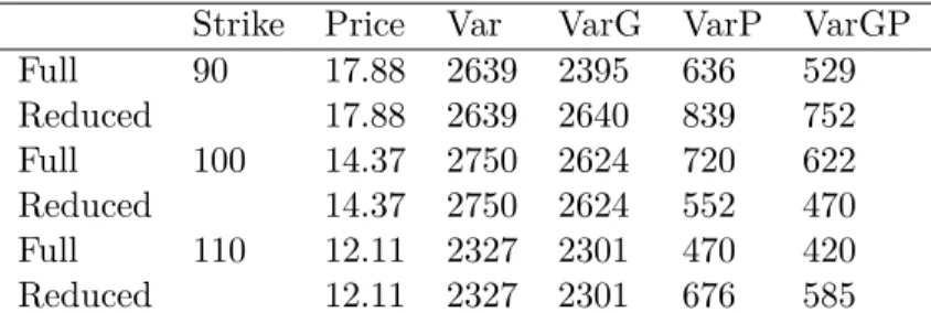
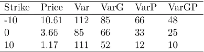
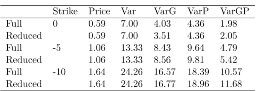
In the following, we compare the efficiencies of several different approaches based on the theoretical part of the paper in the context of option pricing with jumps. The problem always boils down to computing the expectation of a function of a jump diffusion process.