Essays on Macroeconomics

(1)

Washington University in St. Louis

Washington University Open Scholarship

Arts & Sciences Electronic Theses and Dissertations Arts & Sciences

Spring 5-15-2019

Essays on Macroeconomics

Helu Jiang

Washington University in St. Louis

Follow this and additional works at:https://openscholarship.wustl.edu/art_sci_etds

Part of theEconomics Commons

This Dissertation is brought to you for free and open access by the Arts & Sciences at Washington University Open Scholarship. It has been accepted for inclusion in Arts & Sciences Electronic Theses and Dissertations by an authorized administrator of Washington University Open Scholarship. For more information, please [email protected].

Recommended Citation

Jiang, Helu, "Essays on Macroeconomics" (2019).Arts & Sciences Electronic Theses and Dissertations. 1795.

(2)

WASHINGTON UNIVERSITY IN ST. LOUIS Department of Economics

Dissertation Examination Committee: Ping Wang, Chair

Gaetano Antinolfi Sanghmitra Gautam Oksana Leukhina Yongseok Shin David Wiczer Essays on Macroeconomics by Helu Jiang A dissertation presented to The Graduate School of Washington University in

partial fulfillment of the requirements for the degree

of Doctor of Philosophy

May 2019 St. Louis, Missouri

(3)

c

(4)

List of Figures

1.1 Number of Cohabiting Households in the United States . . . 5

1.2 Marriage Status for Females by Education Groups (40-45 years old) . . . 11

1.3 Marriage Status for Females by Education Groups cont. (40-45 years old) . . 12

1.4 Completed Fertility Rate over Time . . . 12

1.5 Completed Fertility Rate over Time by Education Groups . . . 13

1.6 Labor Market for Females . . . 17

1.7 Distributions of h and θ by Education Groups . . . 29

1.8 CPS Data Comparison: March Sample, June Sample, Full Sample . . . 58

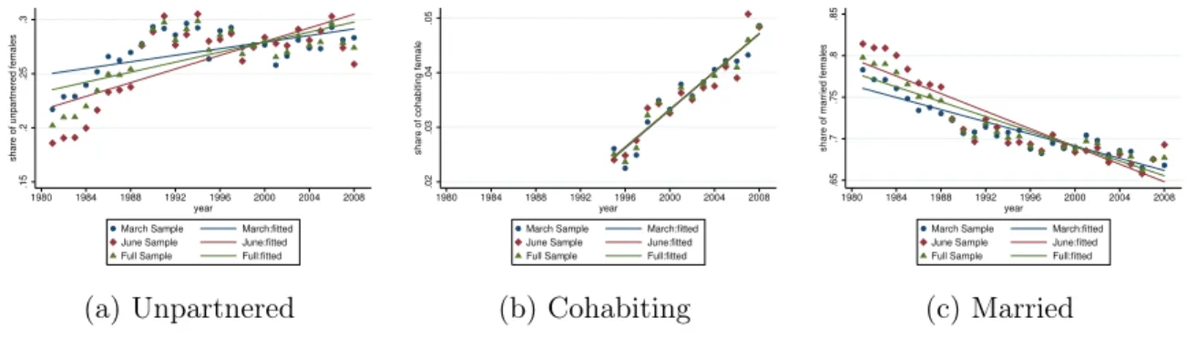
1.9 Share of Unpartnered Females . . . 61

1.10 Share of Cohabiting Females . . . 61

1.11 Share of Married Females . . . 62

1.12 Distribution: Total Hours Usually Spent in Market Work . . . 62

1.13 Distribution: Total Minutes Spent on Child Education Related Activities per Day . . . 63

1.14 Distribution: Total Minutes Spent on Child Education Related Activities per Day . . . 63

1.15 Marriage Status for Females by Education Groups (20-65 years old) . . . 64

1.16 Marriage Status for Females by Education Groups cont. (20-65 years old) . . 65

1.17 Marriage Status for Females by Education Groups (40-45 years old, white) . 66 1.18 Marriage Status for Females by Education Groups (40-45 years old, black) . 66 1.19 Marriage Status for Females by Education Groups cont. (40-45 years old, white) 67 1.20 Marriage Status for Females by Education Groups cont. (40-45 years old, black) 68 1.21 Completed Fertility Rate by Ethnic Groups . . . 69

2.1 Selection into and out of Self-Employment . . . 90

2.2 Skill Premium for Workers and Entrepreneurs . . . 92

2.3 Relative Incomes for Entrepreneurs and Workers . . . 93

2.4 State Level Variation in Worker Skill Premium and Skill Biased Entrepreneurial Decline . . . 95

(8)

2.5 Smoothed Changes in Self-Employment and Real Wages by Skill Percentile . 98 2.6 Smoothed Changes in Entry into Self-Employment by Skill Percentile in

Em-ployment . . . 100

2.7 Density of Entrepreneurial Earnings in the Pooled SIPP . . . 108

2.8 Model and Data Entry Rates relative to 1983 levels . . . 110

2.9 Model and Data Entrepreneurial Skill Premium . . . 111

2.10 Startup Rate in BDS and CPS . . . 113

2.11 Entrepreneurial Dynamics for White Male HH Heads and the rest of sample 116 2.12 Match Rate . . . 118

2.13 Adjusted and Unadjusted Entry and Exit Rates in the Matched March CPS 120 3.1 Comparative Statics . . . 166

(9)

List of Tables

1.1 Changes in Marriage Share, Cohabitation Share, and Fertility Rate . . . 6

1.2 Tendency to have children . . . 14

1.3 Completed Fertility . . . 15

1.4 Time Spent in Market Work and Child Care for Women (40-45 years old) in the United States by Educational Attainment . . . 18

1.5 Time Spent in Market Work and Child Care for Women (40-45 years old) in the United States over Time by Educational Attainment . . . 19

1.6 Calibration parameters . . . 28

1.7 Calibration Target: Marital Shares (Percent), Fertility, and Human Capital Growth Rate for Two Skill Groups . . . 29

1.8 Predicted Marital-Group Fertility for Females . . . 30

1.9 Predicted Contribution to Public Good Production (s) . . . 31

1.10 Counterfactual Experiment 1: Wage and Skill Premium . . . 33

1.11 Counterfactual Experiment 2.1: Effort Cost of Childrearing . . . 34

1.12 Counterfactual Experiment 2.2: Time Cost of Childrearing . . . 35

1.13 Counterfactual Experiment 2.3: Resource Cost of Childrearing . . . 36

1.14 Counterfactual Experiment 3.1: Return of Effort Invested in Children . . . . 37

1.15 Counterfactual Experiment 3.2: Total Return of Investment in Children . . . 38

1.16 Counterfactual Experiment 4: Commitment of Partner . . . 39

1.17 Counterfactual Experiment 5.1: Direct Cohabitation and Marriage Premium 40 1.18 Counterfactual Experiment 5.2: Cohabitation and Marriage Fertility Preference 42 1.19 Dynamics Counterfactual Experiments: Decomposition . . . 45

1.20 Tendency to have children . . . 59

1.21 Completed Fertility . . . 60

1.22 Summary of Counterfactual Experiments . . . 70

1.23 Calibrated Parameters for Two Sub-Periods . . . 71

1.24 Dynamics Calibration Targets . . . 72

(10)

1.26 Dynamics Counterfactual Experiment 1: Wage and Skill Premium . . . 74

1.27 Dynamics Counterfactual Experiment 2.1: Effort Cost of Childrearing . . . . 75

1.28 Dynamics Counterfactual Experiment 2.2: Time Cost of Childrearing . . . . 76

1.29 Dynamics Counterfactual Experiment 2.3: Resource Cost of Childrearing . . 77

1.30 Dynamics Counterfactual Experiment 3.1: Return of Investment in Children 78 1.31 Dynamics Counterfactual Experiment 3.2: Return of Investment in Children 79 1.32 Dynamics Counterfactual Experiment 4: Commitment of Partner . . . 80

1.33 Dynamics Counterfactual Experiment 5: Direct Cohabitation Preference . . 80

2.1 Comparing Polarization in Wages and Entrepreneurship. . . 99

2.2 Testing for Polarization in Entry into Entrepreneurship . . . 101

2.3 Evidence from the SIPP and March CPS . . . 103

2.4 Percentage Change in Self-Employment, Entry and Exit Rate over time.. . . 104

2.5 Model Parameters. . . 109

2.6 Summary Characteristics of Sample . . . 115

2.7 Years of Schooling in March CPS, 1965-2014 . . . 122

3.1 Summary Statistics . . . 137

3.2 Summary Statistics by Skill Groups (Mean) . . . 137

3.3 Summary Statistics by Skill Groups (Median) . . . 138

3.4 Calibration parameters . . . 153

3.5 Model Predictions. . . 154

3.6 Sources of heterogeneity . . . 157

3.7 Fertility preference and leisure loss . . . 158

(11)

Acknowledgments

I am extremely grateful for the help I have received while developing this work. I am deeply indebted to Ping Wang for his patience and continuous support during my years as a PhD student, and will continue to be inspired by his approaches to macroeconomics, and economics in general, in my future research and teaching. I also thank Gaetano Antinolfi and David Wiczer for various discussions on the dissertation. The dissertation were further enriched by comments and suggestions by Yongseok Shin, Oksana Leukhina, Michele Boldrin, Sanghmitra Gautam, Valerio Dotti whom I thank for their involvement too. My research has been influenced by people too numerous to fully acknowledge here, especially since I have had highly stimulating peers, mentors, and friends at WashU, and hence I also want to express my gratitude to the entirety of the WashU economics community in general. Finally, I thank the Department of Economics, Graduate School of Washington University, and the Center for Research in Economics and Strategy (CRES) in the Olin Business School for the financial support.

Helu Jiang

(12)

ABSTRACT OF THE DISSERTATION

Essays on Macroeconomics by

Helu Jiang

Doctor of Philosophy in Economics Washington University in St. Louis, 2019

Professor Ping Wang, Chair

Cohabitation, Marriage, and Fertility: Divergent Patterns for Different Education Groups. The United States has been experiencing a long-term decline in the rates of marriage and fertility and a steady rise in cohabitation. Contradicting the prediction of standard theory that emphasizes the opportunity cost of childrearing from labor market and gender special-ization, skilled females have experienced a less pronounced drop in marriage and fertility, while unskilled females have experienced a more evident increase in cohabitation. I propose the following mechanisms to understand this puzzle: for high-skilled females, the higher im-plicit return of investment in children’s human capital compensates for part of the growing opportunity cost of childrearing; a significant income effect from positive assortative match-ing dominates the conventional wage channel; and when childrearmatch-ing resource cost increases, a strong selection effect exists whereby those with strong fertility motives shift into mar-riage. To quantitatively discipline the relative importance of different factors, I theorize the trade-off between market work and childrearing activities by examining decisions about consumption, marital status, and fertility. Counterfactual exercises show that 34.81%of the rise in cohabitation and 42.42% of the drop in marriage for the skilled can be explained by the rising returns of children, and 38.06% and 40.07%, respectively, for the unskilled. In addition to the returns of children, rising childrearing cost plays a significant role in explain-ing the declinexplain-ing fertility rates, contributexplain-ing to 90.96% and 50.79% of the drop in fertility

(13)

for the two skill groups. Most of the shrinking cohabitation gap and widening marriage gap between the two skill groups can be attributed to the rising wage and skill premium, increasing childrearing costs, and the growing returns of children.

Skill Biased Entrepreneurial Decline. The U.S. is undergoing a long-term decline in the rate of firm startups. We find that this slowdown in entrepreneurship is more pronounced for skilled individuals. In particular, between 1985 and 2015 entry into entrepreneurship declined by 21% for those with at least a college degree and increased by 11%for those with a high school degree or some college experience. We posit that this skill biased entrepreneurial decline is a response to the changing income structure of workers and entrepreneurs that occurred over the same period. In support of this view, we find that, for skilled individuals, entrepreneurial income grew more slowly than worker’s income while for unskilled individuals both incomes grew at relatively similar rates. We also provide evidence for entrepreneurial polarization consistent with wage polarization. To quantify the impact of income structure on entrepreneurial entry we develop a simple heterogeneous-agent, occupational choice model which takes as given a rising worker skill premium, driven by skill biased technical change. In the model, the rising worker skill premium can account for around two-thirds of the changes in entry among skilled and unskilled individuals. This paper contributes to understanding the forces behind the broader decline in business dynamism in the U.S. and suggests an integral role of rising income inequality.

The Timing of Childbearing: Theory and Quantitative Analysis. As significant as the shift from quantity to quality in fertility decisions, a rise in the age at first birth has been commonly observed in the more developed world. This paper attempts to understand such demographic trend both theoretically and empirically. We develop a continuous-time life-cycle model, in which a married woman decides when to have her first child and how she allocates her time to human capital accumulation and market activity. We then calibrate the benchmark model using data from CPS and generalize the model to allow for

(14)

hetero-geneous skill levels. We find that fertility-related productivity loss and job security play a more important role than the conventional human capital channel in terms of explaining the childbearing timing differentials between skill groups, and women are more sensitive to changes in fertility preference as opposed to leisure loss. Compared with high-skilled women, low-skilled women are more vulnerable to changes in labor productivity, human capital, hus-band’s income, utility derived from children and the disutility in raising children. As a result, low-skilled women push up or defer their timing of childbirth more relative to high-skilled women.

(15)

Chapter 1 Cohabitation, Marriage, and Fertility:

Divergent Patterns for Different

Education Groups

Helu Jiang

1.1 Introduction

The United States has experienced significant behavioral changes that affect the family structures over the past few decades: the rates of marriage and fertility have dropped dra-matically, accompanied by a pronounced increase in cohabitation. This paper documents the puzzle in divergent marital and fertility patterns between skill groups, finding that the decline in marriage and fertility is less dramatic for high-skilled females while the rise in cohabitation is more dramatic for low-skilled females. To understand the underlying driving forces leading to such differences, I build a model that features trade-offs between private consumption, public good consumption, and utility from children in which marital choices

(16)

and fertility decisions are determined jointly.

Many early discussions have been focused on the increase in the age at first marriage, greater instability leading to “retreat from marriage" and delay in childrearing decisions. However, one striking fact that is often ignored is the rising trend of cohabitation. Figure1.1, borrowed fromFitch et al.(2005), shows the number of cohabiting households nearly doubled from 1960 to 1970, and now, cohabitation has become a common living arrangement1. It is of great importance to take cohabitation into consideration when studying family structures. Moreover, using data from the Current Population Survey, I find that skilled females with at least a bachelor’s degree have experienced a less pronounced drop in marriage and fertility rates, while unskilled females have experienced a more evident increase in cohabitation, as shown by Table 1.1. In the 1980s, 79.8%percent of unskilled females aged between 40 to 45 years old were currently married; this number dropped to 64.3%in 2008; for the skilled, the marriage share declined from 80%in 1980 to 74.9%in 2008; fertility dropped by 23.5% and 15.6%, respectively, over the same period. Cohabitation increased from 2.82%and 1.75%in 1995 to 5.63% and 3.41% in 2008 for the skilled and the unskilled. These facts challenge the standard theories that emphasize the opportunity cost of childrearing from labor market and gender specialization.

The traditional theory, stemming from Becker’s sequences of work2_{, emphasizes the}

sources of gains of marriage from specialization and posits that marriage is rationalized as a lifetime contract between a man and a woman, in which the man performs market work while the woman performs home production. As an increasing number of women is able to get access to higher education and participate in the labor market and the gender gap narrows3, marital surplus falls with reduced specialization. In response to these underlying

1_{POSSLQ means Persons (or Partners) of Opposite Sex Sharing Living Quarters.} 2_See_Becker _(1973),_Becker _(1974),_Becker _(1981).

3_{Blau and Kahn}_{(2017) provides a thorough review of the trends and explanations of evolution of gender}

(17)

changes in the economy, the divorce rate has also been increasing, along with the declining marriage rate and fertility rate (Lundberg et al., 2016). However, although the standard theories can explain the aggregate trends of declining marriage and fertility and rising co-habitation, they cannot fully explain the puzzle in divergent marital and fertility decisions between skill groups.

The rising income inequality between college-educated individuals and non-college-educated ones implies that high-skilled females not only face a higher opportunity cost of childrearing and a lower gender specialization gain from marriage, but they also experience a growing opportunity cost and a decreasing benefit from marriage. In this case, singlehood and cohab-itation should have become more desirable for the skilled. Not only the wage gap is widened, but the income volatility also increases, especially for the less-educated households4_{. Facing}

a more volatile income stream, the unskilled should have found it more attractive to live with a partner for risk-sharing purposes than the skilled. Hence, it is often taken for granted that there should be more educated females who are less likely to get married or have children, which is contradictory to the divergent patterns found in data.

To understand the puzzle of the divergence of marital shares and fertility rate between skill groups, I propose the following four important mechanisms. First, a higher return of investment in children’s human capital partly compensates for the high opportunity cost of childrearing for the skilled, and thus the skilled face a trade-off between external return from the labor market and implicit return from investment in children’s quality. Data from the American Time Use Survey support this claim that educated women not only spend more time working in the outside labor market, but also invest more time in their children. Over the 2003 to 2006 period, the growth rate of time spent on childcare also increases with edu-cational attainment. Second, the income effect from positive assortative matching dominates

4_{Dynan et al.} _{(2012) claim that households including individuals who do not a college degree have}

consistently experienced more volatile incomes than households with members who have a college degree. More importantly, increases in income volatility are somewhat greater among less-educated households.

(18)

the conventional gender specialization effect for the skilled. Unlike low-skilled females, who retreat from marriage to cohabitation when facing a higher wage rate that is predicted by the conventional wage channel, high-skilled females benefit more from assortative mating because of income effect, and this increases the attractiveness of marriage when wages rise. Third, as childrearing cost goes up, the low-skilled group shifts from marriage to cohabita-tion and has fewer children. Nevertheless, seleccohabita-tion effect is strong for the high-skilled group that those who have really strong fertility motives deviate from singlehood or cohabitation to marriage because the benefit associated with childrearing activities in marriage status will offset part of the increase in the cost. Last, marital and fertility decisions will also be affected by the level of the potential partner’s commitment and people’s preference toward different living arrangements. How much the partner contributes to the household will affect a female’s choice on family formation. Skilled females and unskilled females may react dif-ferently to a change in the partner’s commitment level because of different utility associated with public good consumption. Moreover, changes in legal treatments aiming to protect vulnerable parties in cohabiting relationships increase the acceptance of cohabitation.

In the model, female agents are heterogenous in their skill type, human capital, and type of potential partner they will meet. They choose their marital status and the number of children they want to have and allocate their time and resources to labor work, public good production, and educating children. The matching market is exogenous that a positive assortative matching process is assumed. The efficiency of investment in children’s human capital will depend not only on the female’s own human capital and effort invested, but also on choices of marital status. Turning to the quantitative analysis, I calibrate the benchmark model to the U.S. economy by targeting average marital shares and fertility rate for two skill groups from 1995 to 2008. The model can well capture the within-skill-group fertility rates in different marital statuses and between-skill-group fertility differentials. Two sets of counterfactual experiments are performed. The first set is designed to understand how

(19)

different factors affect two skill groups differently. It is important to see the interactions of income effect, substitution effect, quantity-quality trade-off, and selection effect. The second set of experiments is conducted in a dynamic setting in which I divide the sample into two sub-periods and restore the value of parameters of interest in the second sub-period to its value in the first sub-period. Counterfactual exercises show that rising childrearing cost and return in children play a significant role in explaining the declining fertility rates for two skill groups. In terms of changes in marital shares, return in children contributes to 34.81%

of the rise in cohabitation and 42.42% of the drop in marriage, and 38.06% and 40.07%, respectively, for the unskilled. In addition, high-skilled females are more sensitive to rises in their partners’ commitment and cohabitation preference, while low-skilled females are more vulnerable to rises in wage and childrearing cost. Because of the higher return of investment in children’s quality, higher benefit from positive assortative matching, and strong selection effect faced by the skilled, rising skill premium and childrearing costs have opposing effects on the two skill groups. The shrinking cohabitation gap and widened marriage gap between the two skill groups are largely explained by the rising wage and skill premium, increasing childrearing costs, and growing return in children. Three channels together contribute to around 165.8% of the increasing marriage differentials between skill groups, and partners’ commitment together with cohabitation preference attributes to negative 65.8%.

(20)

Figure 1.1: Number of Cohabiting Households in the United States

Source: Fitch et al. (2005)

Table 1.1: Changes in Marriage Share, Cohabitation Share, and Fertility Rate

Marriage (1980-2008) Cohabitation (1995-2008) Fertility (1980-2008)

High-skilled -6.39% 94.81% -15.59%

Low-skilled -19.46% 100.06% -23.50%

Source: CPS June Supplement

1.1.1 Literature

This paper is related to several themes of research. The first related field is the study on economics of marriage and the evolving role of marriage. Back in the 1970s, Gary Becker (Becker (1973), Becker (1974)) developed the economic model of marriage. He rationalized the marriage between a man and a woman as a lifetime contract in which the man provides income from market work and the woman provides household work such as cooking, childcare, and house cleaning. The expected source of gains of marriage stemmed from specialization and exchange (Becker, 1981). Later work has recognized gains from joint consumption of public good such as children and housing (Lam, 1988). Another approach to the study of

(21)

marriage is the bargaining model. For example,Manser and Brown(1980) and McElroy and Horney (1981) developed the divorce-threat bargaining model, in which distribution within the marriage is treated as the solution to a cooperative game, the threat point of which is usually divorce. Empirically, Lundberg and Pollak (2015) investigated the evolving role of marriage in the United States. Since the focus of this paper is not on the distribution within marriage or the matching process between two parties, similar to De La Croix and Doepke (2003) andDoepke(2004), I follow a more macro approach by modeling the choices of female agents, abstract from matching market.

In most early works, cohabitation is not explicitly considered a possible living arrange-ment. Empirically, it is also hard to measure cohabitation due to data limitations. Re-searchers at the Census Bureau started developing national representative estimates of the number of cohabiting couples in the late 1970s (Glick and Norton (1977),Glick and Spanier (1980), Glick (1984), Bumpass and Sweet(1989b)). The measure known as Partners of the Opposite Sex Sharing Living Quarters (POSSLQ) was developed to infer cohabiting couples indirectly from the data. Later Casper and Cohen (2000) refined this measure into the ad-justed POSSLQ to improve the estimates. Later in the 1980s and 1990s, with more data available, researchers started to investigate the emergence of cohabitation using either direct measures or indirect inference tools. Manning(2013) provides a detailed review of the related empirical literature. Not until 1995 did the CPS start to report cohabitation information by providing the relationship of an individual to the head within the same household5_{. CPS}

data provide a more precise measure for cohabitation than using POSSLQ. For example, from the survey questions, now it is possible to differentiate cohabiting couples from room-mates sharing a space. Another stream of literature that studies cohabitation investigates the wealth accumulation (Vespa and Painter, 2011), happiness, and influence of different

5_{This paper only considers opposite-sex cohabiting and married couples. I understand that it is important}

to study same-sex partners, but this is not my main interest since less than 2&of unmarried couples are same-sex in the original data set.

(22)

family structures on children (Thornton (1988),Bumpass and Sweet (1989a), Bumpass and Lu (2000)). I contribute to this literature by studying the puzzle of divergence of marital choices between skill groups, and I take cohabitation as a serious living arrangement as opposed to singlehood and marriage.

An important focus of this paper is people’s fertility decisions, including both the intensive and the extensive margins. I not only study whether a female decides to have kids or not, but also study the quantity and quality trade-off. Advanced byBecker(1960),Becker(1973), and Willis (1973), economists who study modern economic demography concentrate on parental trade-offs between the number and quality of children. Hanushek (1992) provides empirical evidence that family size directly affects children’s achievement. This paper contributes to the theory by providing a new channel that considers the return of investment in children’s human capital to explain different behaviors across skill groups. To reinforce this idea, educated females face a high opportunity cost of childrearing and enjoy a high return of educating their kids, thus leading to a trade-off between market work versus childbearing activities.

This work is also related to studies on inequality, gender gaps, and female labor market performance. Barro and Becker (1989) apply the framework of altruistic parents making choices about family size together with consumption decisions and intergenerational transfers to a closed economy, extending the optimal economic growth literature by allowing optimal choices about fertility and intergenerational transfers. Galor and Weil(1993) link the gender gap with fertility and investigate the impact on aggregate growth in the economy. Although my paper is not directly discussing economic growth, it is essential to study how labor market conditions and rising inequality affect women’s choices on family formations. Several recent papers discuss that marital and fertility patterns differ among different groups. Greenwood et al. (2016) document that the drop in marriage and the increase in divorce are greater for non-college-educated individuals versus college-educated ones. They construct a unified

(23)

model of marriage, divorce, educational attainment, and female labor force participation. However, cohabitation and fertility are not part of the picture, which are the major focus of this paper. Bar et al. (2018) study the flattened relationship between income and fertility, proposing the marketization of parental time costs as the driving force. They focus on the income effect for the high-income women and marital sorting. What is different in this paper is that an assortative matching process is assumed to be fixed overtime. I want to avoid getting into the debate about whether such assortative mating has increased. The income effect increases the attractiveness of marriage for high-skilled females because of the positive assortative matching. This paper has shed light on understanding how income inequality and changes in labor market conditions shape females’ decisions about family structures and fertility.

The most closely related paper is by Lundberg et al. (2016). They use data from 1960-2000 U.S. censuses and 2010 American Community Survey to document divergent patterns in marriage, cohabitation, and childbearing. They also discuss the changes in gender roles, marital surplus, and investments in children. Two crucial aspects of this paper are different from theirs. First, in the empirical part, I restrict the sample to females aged from 40 to 44 because this paper focuses on lifetime choices instead of dynamic transitions and I believe this age restriction better captures the completed fertility. Second,Lundberg et al. (2016)’s paper is an empirical work. In contrast, I develop a theory to rationalize the importance of return of investment in children’s quality. By performing counterfactual experiments, I am able to determine the relative importance of different forces behind the model.

1.2 Empirical Findings

I follow Lundberg et al. (2016) in considering only high school graduates and those with bachelor’s degrees or above. To be more specific, the low-skilled group is defined as the

(24)

sample of females with high school degrees, including individuals with some college experience but no bachelor’s diploma. The high education group is defined as women with at least a bachelor’s degree. I further restrict the sample to females aged between 40 to 44 since this age group is close to the end of females’ fecundity cycle, thus providing a more precise measure for completed fertility rate. For the majority of the empirical results, I take data from the Current Population Survey (IPUMS CPS)6. I focus on the time periods starting from 1980 to 2008. Year 1980 is the earliest year for which I can get reliable data, and year 2008 is chosen as the ending period because the Great Recession is not the focus of this paper. Not until year 1995 did cohabitation data become available, and hence any analysis using cohabitation data starts from that year.

I first present empirical findings on divergent marital choices and fertility decisions tween low-skilled and high-skilled groups, and then I provide evidence on the trade-off be-tween outside opportunity cost of childbearing working in the labor market and implicit return of investment in children.

1.2.1 Evolution of Marital Status

Figure 1.2 and Figure 1.3 illustrate the evolution of marital choices by education groups. In the 1980s, 79.85%percent of unskilled females aged between 40 to 45 years old were currently married; in 2008, this number dropped by 19.46% to 64.31%; for the skilled, the marriage share declined by 6.39% from 80.01% in 1980 to 74.90% in 2008. The cohabitation share rose from 2.82% and 1.75% in 1995 to 5.63% and 3.41% in 2008 for the unskilled and the skilled, and the increase was 99.65% and 94.86%, respectively. Despite the fact that both skill groups have experienced a sharp drop in marriage and a steady rise in cohabitation, the changes are more dramatic for the unskilled.

The group “unpartnered" is defined as the union of females who are currently separated,

(25)

divorced, or widowed and females who have never married, also denoted as "single" in this paper. The declining rate of being unpartnered for the highly educated females is mostly driven by the declining rate of being separated, divorced, or widowed because the single share posits a positive trend. The divergent pattern is observed here that the single share rose from 3.89% to 11.13% for the unskilled, and this increase is much less dramatic than that for the unskilled, which grows from 7.55%to 10.32%7.

Figure 1.2: Marriage Status for Females by Education Groups (40-45 years old)

.01 .02 .03 .04 .05 .06

share of cohabiting females

1980 1984 1988 1992 1996 2000 2004 2008 year

low:cohabiting fitted value high: cohabiting fitted value

(a) currently cohabiting

.6

.65

.7

.75

.8

share of married females

1980 1984 1988 1992 1996 2000 2004 2008 year

low:married fitted value high: married fitted value

(b) currently married

Source: June CPS Supplement

1.2.2 Evolution of Fertility

Next, let us look at the evolution of fertility rates over time. Fertility rate is defined as the average number of children ever born over the female sample aged between 40 and 44 years old conditional on having at least one child8_{. Figure}_1.4 _{shows the declining aggregate trend}

7_Appendix_1.9.2_{provides figures on detailed evolution of marital status by fertility decision.}

8_{There are multiple ways to calculate fertility rates. Completed fertility is the average number of children}

born to women belonging to the same cohort once they have reached the end of their reproductive life. General fertility is defined as births per 1000 women aged over the total female sample. Total fertility is the hypothetical lifetime births per woman. Completed fertility is chosen here because (1) this age group is toward the end of a female’s fecundity cycle, (2) fertility questions in the CPS June Supplement are asked of females aged 15-44 years old in most sample periods of interest, (3) childrearing timing decision or marital status transition is not my main interest, and (4) the zero-mass issue is not a major emphasis in this paper.

(26)

Figure 1.3: Marriage Status for Females by Education Groups cont. (40-45 years old)

.2

.25

.3

.35

share of unpartnered females

1980 1984 1988 1992 1996 2000 2004 2008 year

low: unpartnered fitted value high: unpartnered fitted value

(a) currently unpartnered

.1

.15

.2

.25

share of separated, divorced, or widowed females 1980 1984 1988 1992 1996 2000 2004 2008 year

low: SDW fitted value high: SDW fitted value

(b) currently separated, divorced, widowed

.04

.06

.08

.1

.12

share of females never married

1980 1984 1988 1992 1996 2000 2004 2008 year

low: never married fitted value high: never married fitted value

(c) never married (single)

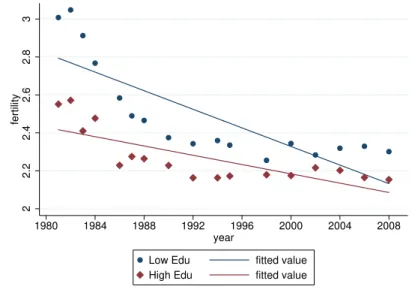
of fertility. The left panel is the naive measure, while the right panel shows the average predicted fertility from the OLS regression in which I control for a quartic in age, education, experience, race dummies, state dummies, and industry dummies. A more detailed report of changing rates of fertility by education groups can be seen in Figure 1.5. The fertility rate dropped by 23.5%from 3 to 2.3 and 15.6%from 2.6 to 2.2 for the two skill groups conditional on having children. Again, despite the common declining rates in fertility experienced by two skill groups, the drop is more dramatic among the low-skilled.

(27)

Figure 1.4: Completed Fertility Rate over Time 2 2.2 2.4 2.6 2.8 3 fertility 1980 1984 1988 1992 1996 2000 2004 2008 year

fertility fitted value

(a) naive measure

2 2.2 2.4 2.6 2.8 3 fertility 1980 1984 1988 1992 1996 2000 2004 2008 year

fitted fertility fitted value

(b) regression measure

Figure 1.5: Completed Fertility Rate over Time by Education Groups

2 2.2 2.4 2.6 2.8 3 fertility 1980 1984 1988 1992 1996 2000 2004 2008 year

Low Edu fitted value High Edu fitted value

1.2.3 Fertility Choice vs. Marital Decision

The previous two sections document the fact that the two skill groups posit different trends of evolution in family structures and fertility decisions. This section shows that it is important

(28)

to understand that decisions about living arrangements and childrearing are closely related. Table 1.2 and Table1.3 examine how fertility choice is related marital decision9_.

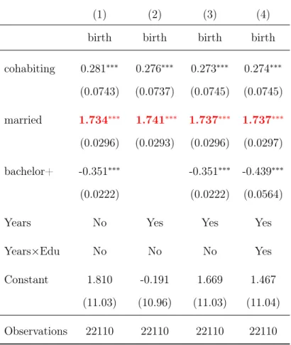
In Table 1.2, the average marginal effect from the PROBIT regression on whether a woman has at least one child or not is reported, with age, a quartic term in age, occupation, industry, race, and state dummies controlled. The coefficients in the first and second row imply that compared to single females, females who choose cohabitation are more likely to have at least one child, and married females have the highest probability of having children after controlling for demographic characteristics.

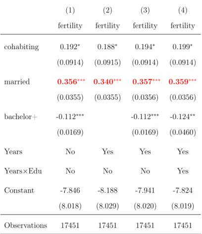
Table 1.3 reports the results from the OLS regression on fertility rate controlling for the same demographic variables. Conditional on having at least one child, married females tend to have the highest number of children among the three marital groups, and cohabitation group comes second. Although a strict casual relationship cannot be achieved from these two tables, the results imply that fertility decisions and marital choice are interrelated in the sense that people with various fertility motives may choose different living arrangements, and vice versa. Therefore, it is of great importance to study childrearing decisions and choices of different marital status together as a joint decision process.

9_{See Table}_1.20 _{and Table} _1.21_{in appendix} _1.9.2_{for the results using being unpartnered as the base}

(29)

Table 1.2: Tendency to have children

(1) (2) (3) (4)

birth birth birth birth

cohabiting 0.281∗∗∗ 0.276∗∗∗ 0.273∗∗∗ 0.274∗∗∗ (0.0743) (0.0737) (0.0745) (0.0745) married 1.734∗∗∗ _1.741∗∗∗ _1.737∗∗∗ _1.737∗∗∗ (0.0296) (0.0293) (0.0296) (0.0297) bachelor+ -0.351∗∗∗ -0.351∗∗∗ -0.439∗∗∗ (0.0222) (0.0222) (0.0564)

Years No Yes Yes Yes

Years×Edu No No No Yes

Constant 1.810 -0.191 1.669 1.467

(11.03) (10.96) (11.03) (11.04)

Observations 22110 22110 22110 22110

Standard errors in parentheses

(30)

Table 1.3: Completed Fertility

(1) (2) (3) (4)

fertility fertility fertility fertility cohabiting 0.192∗ 0.188∗ 0.194∗ 0.199∗ (0.0914) (0.0915) (0.0914) (0.0914) married 0.356∗∗∗ 0.340∗∗∗ 0.357∗∗∗ 0.359∗∗∗ (0.0355) (0.0355) (0.0356) (0.0356) bachelor+ -0.112∗∗∗ -0.112∗∗∗ -0.124∗∗ (0.0169) (0.0169) (0.0460)

Years No Yes Yes Yes

Years×Edu No No No Yes

Constant -7.846 -8.188 -7.941 -7.824 (8.018) (8.029) (8.020) (8.019) Observations 17451 17451 17451 17451

Standard errors in parentheses

∗ _{p <}₀_.₀₅_,∗∗_{p <}₀_.₀₁_,∗∗∗_{p <}₀_.₀₀₁

There are three takeaways from these empirical results: (1) on average, regardless of marital status, unskilled females tend to have more children than skilled females; (2) the fertility rate has dropped much less for skilled females; (3) divergence also appears in marital choices between two skill groups in that both the drop in marriage and the rise in cohabitation are more prominent for unskilled females. The first observation is consistent with quantity-quality trade-off theory that high-skilled females with higher incomes are more likely to invest in the quality of their children rather than the quantity. However, the puzzle comes from the second and the third observations, namely the divergence between the two skill groups.

(31)

In the next two sections, I show that it is true that women now face a much higher opportunity cost of childbearing, and those with higher skills suffer an even higher cost because of rising skill premium. Nevertheless, females gain an implicit return from investing time with their children, although such a return may depend on different family structures. Therefore, females face a trade-off between outside opportunity cost and implicit return of investment in children’s human capital, thus providing a novel channel to understand the puzzling different trends of marital shares and fertility rate between skill groups.

1.2.4 Labor Market for Females

I followAcemoglu(2002) in constructing the skill premium for females. The relevant measure of a worker’s income is constructed from the IPUMS variables INCWAGE, which is the annual income reported in real 2010 USD. Those with no earnings and the remaining lowest 1 percent of earners are dropped from the sample. Top-coded incomes are assumed to be 1.5 times the top-code. The reported measure of skill premium is the coefficient on a dummy variable for those with at least a bachelor’s degree (compared to those with only a high school degree or some college experience) in an OLS regression of log income with a variety of controls. The controls are (1) a quartic in years of potential experience, (2) race (white/non-white) dummy, (3) state dummies, and (4) additional dummies for educational categories. Years of potential experience E = age−S −6 is defined by assuming that an individual’s schooling starts after age six. Years of schooling, S, are assumed using the IPUMS variable EDUC. This variable reports the highest level of educational attainment of a respondent.

Figure 1.6 reports the changes in labor market for females from 1980 to 2008. Panel (a) illustrates the rising share of females who have higher education experience. The share of the high-skilled increased from 13.36% in 1980 to 35.33% in 2008. Panel (b) illustrates the striking increase in female labor market participation rate in that more and more women have

(32)

engaged in market work. This features a decreasing gender pay gap and less discrimination (Hsieh et al., 2013). Panel (c) shows the rising skill premium. Higher return on skills leads to even higher outside cost for skilled females. Easier access to higher education and better labor market conditions imply that an increasing number of females are able to earn a higher return from the labor market; however, this also implies a higher opportunity cost of childrearing.

Figure 1.6: Labor Market for Females

.2 .25 .3 .35 share 1980 1984 1988 1992 1996 2000 2004 2008 year

share of high skill females fitted values

(a) college+share

52 54 56 58 60 62 share 1980 1984 1988 1992 1996 2000 2004 2008 year

female labor market participation rate

(b) participation rate 1.3 1.4 1.5 1.6 1.7 skill premium 1980 1984 1988 1992 1996 2000 2004 2008 year skill premium (c) skill premium

Source: CPS March Supplement and FRED

1.2.5 Time Spent on Kids

Return of investment in children could take multiple forms: spending time with kids might give direct utility to parents, or some parents just love to be with their children; parents may care about the future income/future job/education of their children; and parents may directly get monetary support from their children. Hence, it is very complicated to measure such intangible implicit return of investment in children. Instead, here I provide supporting evidence of the time spent on children since it reflects how parents value time invested in different activities.

(33)

Table 1.4: Time Spent in Market Work and Child Care for Women (40-45 years old) in the United States by Educational Attainment

Marital Status Market Work, hours/week Childcare, minutes/day Education Unpartnered Cohabiting Married total hours main job caring education health total

high school 27.47% 4.46% 68.06% 25.512 23.229 29.757 8.942 1.092 39.794

some college 30.18% 3.88% 65.94% 29.288 25.893 39.036 12.743 2.690 54.586

BA and above 23.14% 2.92% 73.94% 30.017 26.591 62.158 15.303 2.141 79.648

Using the American Time Use Surveys from 2003 to 2008, I examine parental time allocated to childbearing activities10_{. As Table} _1.4 _{shows, both the time spent on market}

work and childcare increases with years of schooling11_{. This is also supported by} _Guryan

et al. (2008), who claims the relationship still holds even when controlling for employment status. He found that mothers with at least a bachelor’s degree spend approximately 4.5 hours more per week on childcare than mothers with a high school degree or less. Given the fact that the higher-educated parents also spend more time working in the labor market, the striking finding that they are also more likely to spend time with their child/children implies that there must exist an implicit higher return for time invested in their children.

10_{Childcare activities include physical care for children, reading to/with children, playing with children}

(not sports), arts and crafts with children, talking with/listening to children, organization and planning for children, looking after children, attending children’s events, waiting for/with children, picking up/dropping off children, and caring for/helping children. Activities related to household children’s education include homework, meetings and school conferences, home schooling, and waiting associated with children’s edu-cation. Activities related to household children’s health include providing medical care, obtaining medical care, and waiting associated with children’s health. SeeBLS websitefor more information.

(34)

Table 1.5: Time Spent in Market Work and Child Care for Women (40-45 years old) in the United States over Time by Educational Attainment

total hours usually worked per week total minutes spent on childcare per day

year high school some college BA and above high school some college BA and above

2003 26.15 28.25 28.54 53.62 52.43 79.33 2004 26.63 29.57 29.30 32.74 53.21 74.97 2005 26.79 28.91 30.43 33.92 54.38 84.42 2006 24.36 30.06 31.83 38.89 55.34 69.25 2007 24.30 29.01 29.27 41.95 58.06 82.20 2008 24.23 30.10 30.53 37.27 54.60 87.40 change -7.35% 6.52% 6.96% -30.48% 4.15% 10.18%

What is more, over this period, high school graduates decrease both time spent in market work and time in childcare; on the contrary, females with at least some college experience devote more time into labor work and invest more in their children. As can be seen from the last row in Table 1.5, the growth rate of time spent on childcare also increases with educational attainment. Facing a higher wage and rising skill premium, the skilled females find it more profitable to work for longer hours in the market. At the same time, the fact that they also increase the time they spend on childcare implies that return from investment in children for the skilled is not only higher but also increases faster than that for the unskilled.

1.3 Benchmark Model

Female agents in the model are assumed to be heterogenous in three aspects: skill type, human capital, and type of potential partner. There are two skill groups in the economy,

(35)

high-skilled (college-educated) or low-skilled (non-college-educated). 1col =       

1 high skill group denoted by H

0 low skill group denoted byL

Within each skill group, agents are endowed with human capitalh, following the distribution of human capital denoted byFH(h)andFL(h), respectively. In addition to the skill type and human capital, an agent is also endowed with an exogenousθ that governs the income of her potential partner, exogenously drawn from distributionsGH₍_θ₎_{, and} _GL₍_θ₎_{. I abstract from}

the double-sided marriage market and assume the positive assortative matching process. Hence, the exogenous state of a female agent in the model can be described by (1col_{, h, θ}₎_.

In the model, each agent is endowed with one unit of time, and she values utility from private good consumption, utility over her children’s human capital discounted by total number of children, and utility from public good consumption if she is in cohabitation or marriage status. She allocates the one unit of time to childrearing activities and working in labor market, and part of her labor income will be used for public good production if she chooses to cohabit or marry a partner. To summarize, she makes decisions about consumption (c), the lifetime quantity of children (n), effort invested in children’s human capital (q), resources allocated to public good production (s), and public good consumption (X) with a subsistence level of consumption (X). All these choices are continuous.

Raising a kid takes time and money. Hence, I model both the resource cost and time cost, denoted byπ0 andπn, respectively. Educating a kid is a time-intensive activity. I denote the

time cost by πq. There would be a trade-off between quantity and quality of children. The

human capital accumulation process for children depends on the parents’ own human capital and the effort they invest in educating their children. Production of public good requires labor income contribution both from the female agent and her partner.

(36)

At the same time, the agent makes a discrete choice on marital status, including single-hood, cohabitation, and marriage, denoted by M ∈ {s, c, m}. To simplify notations, I also use three indictor functions to capture the endogenous marital decision: 1s _{= 1} _represents

being single, 1c _{= 1} _{cohabiting with a partner, and} 1m _{= 1} _{being married. The model is}

static in the sense that there is no breakup or divorce12_.

1.3.1 Household Utility

Omitting the subscript for individual i, the utility function of a female agent endowed with

(1col_{, h, θ}₎ _{is defined as follows:}

U = c 1−σc 1−σc + (1M ·αM_n )nγ(nh 0₎1−σn 1−σn +1Mδ_nM +1c·αX (X−X)1−σX 1−σX +1m·αX (X−X)1−σX 1−σX ·(1 +1cδc+1mδm) (1.1)

The utility function is assumed to take CRRA functional form, and the intertermporal pref-erence parameters in the CRRA utility function are assumed to vary for private consumption (σc), children (σn), and public good (σX).

All female agents in the model can choose to have kids. They decide how many children to have, and they care about the quality of their children. Hence, utility over children contains two parts: total human capital from children (nh0) and a fertility utility premium (δM

n ). Following Becker et al.(1990), I assume both will be discounted by the total quantity

of children that is governed by the parameterγ. The fertility utility premium is modeled to capture the fact that even if a parent does not invest any effort into children’s human capital development, the presence of children will bring her happiness, although such happiness decreases with the number of children. Both fertility preference parameter α_nM and fertility premium δM

n are assumed to vary across different marital statuses such that αsn < αcn ≤αmn 12_{Note that variables or parameters with superscript} _{_{s, c, m}_} _{imply that they are specific to marital}

(37)

and δs

n < δnc ≤ δnm, which is supported by the empirical evidence shown in section 1.2.3

that females who choose different living arrangements are associated with different fertility motives.

Cohabiting and married females are assumed to face the same public good preference parameterαX, while single women do not have the choice of enjoying public good. The

sub-sistence level of public good consumption captures the idea of necessary joint expenditure for two partners, such as housing. Although there is no breakup or divorce in the model, direct utility cost/premium parameters δc and δm capture the net direct utility from cohabitation

and marriage. For example, a negative δm implies that the cost associated with marriage,

such as wedding cost or divorce cost, outweighs the benefit from marriage. The important point is that I do not put any parametric restrictions on these two parameters, and in the calibration part, I will let the model tell.

1.3.2 Budget Constraint

A skilled female worker gets a unit wage of ωH _{while an unskilled worker gets a unit wage}

of ωL_{. The total wage a female agent gets is proportional to her own human capital.}

w=ωh

= [1colωH + (1−1col₎_ωL_]_h

The exogenous assortative matching process implies that if a female gets wage w, then she will meet a partner who earns θw. The budget constraints are written as follows:

c=w(1−s)·

1−(1sπs_q+1cπ_qc+1mπ_qm)qn−πnn

(38)

where πn=1colπHn + (1−1 col₎_πL n π0 =1colπH0 + (1−1 col₎_πL 0

1.3.3 Human Capital Accumulation Process

Children’s human capital partially depends on how smart their parents are and partially on how much effort their parents invest. Parameters τ and η capture the relative importance nature versus nurture plays in shaping a person’s human capital. Efficiency in educating children depends on family structures, which contention is supported by a vast of empirical literature13. Hence, I assumeκs < κc≤κm.

h0 =H(q, h) =B·hτ ·(κM +q)η (1.3)

where

B =1colBH + (1−1col₎_BL 1> τ, η >0, τ +η≤1

1.3.4 Public Good Production

If a female agent decides to cohabit with or marry a partner, she can enjoy a public good with her partner, but she needs to allocate fractionsof her market work value to public good production. Simultaneously, her partner contributessM

manportion of his incomewman =θ·w

to public good production. Nevertheless, if a female agent chooses singlehood, she does not

13_{There is a considerable amount of empirical literature that documents the benefits of marriage for the}

well-being of children. On average, children living with two biological married parents tend to experience better educational, cognitive, and social outcomes not only in the short-term but also through adulthood (Artis(2007),Broman et al.(2008),Brown(2004),Carlson and Corcoran(2001),Manning and Lamb(2003), Teachman (2008), Videon(2002), Amato (2005)). Several works have also been conducted to use theories to explain the relationship between family structures and the well-being of children. Potential theoretical explanations include economic resources, parental socialization, family stress or turbulence, and selection

(Amato (2005), Carlson and Corcoran (2001),Huston and Melz (2004)). See Brown(2010) for a detailed

(39)

have the option to consume public good. Production of public good takes the following form:        Xc ₌ [ws(1−πc qqn−πnn)]ρ c + (wmanscman)ρ c 1 ρc_/ξ Xm ₌ [ws(1−πm q qn−πnn)]ρ m + (wmansmman)ρ m 1 ρm_/ξ (1.4)

Notice that ξ captures the possibility for a female to meet a partner with negative asset (positive debt or liability) even if the partner has a positive income value. I assume ξH =

ξL= 2 for the benchmark case.

1.3.5 Maximization Problem

The maximization problem can be solved in two steps. First, conditional on marital sta-tus, a female agent chooses private consumption c, number of children n, effort invested in children’s human capital q, fraction devoted to public good production s, and public good consumptionX to maximize utility (equation1.1) subject to the budget constraint (equation 1.2), facing human capital accumulation process of their children (equation 1.3), and public good production (equation1.4). Then she compares the total utility when choosing different marital status including singlehood, cohabitation, and marriage, and then she will choose the one that gives her the highest utility (M∗). The formal maximization problem is written

(40)

as follows:

step1: V(M) = max

c≥0,n≥0,q≥0,1≥s≥0,X≥XU

subject to

budget constraint (1.2)

human capital accumulation process for children (1.3)

public good production(1.4)

step2: M∗ = argmax

M∈{s,c,m}

V(M)

1.4 Calibration Strategies and Results

Since data on cohabitation in the CPS did not become available until year 1995 and the emphasis of this paper is not on the Great Recession, I only consider the time period from year 1995 to year 2008.

For potential partner’s income and contribution to the production of public good, I assume the following functional forms that the time a partner contributes to the public good will be proportional to the time the female agent contributes:

wman =ωh·θ =ωh·[1colθH + (1−1col)θL]

sc_man=s(1−π_qcqn−πnn)·scman

sm_man=s(1−πm_q qn−πnn)·smman

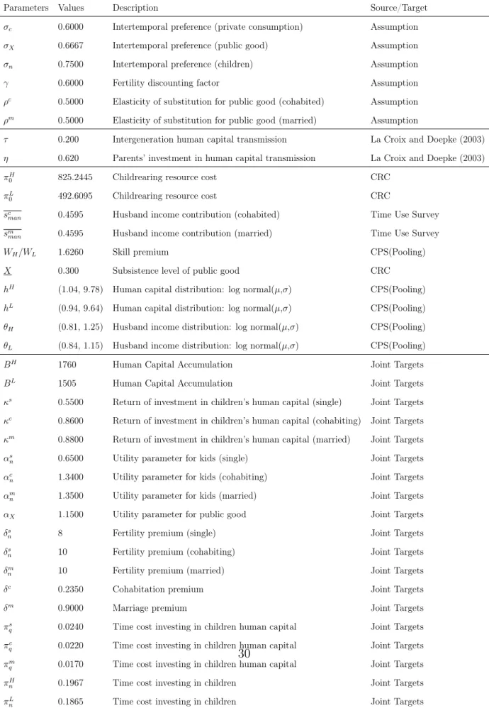
There are thirty-seven parameters in total, out of which two parameters will be taken from the existing literature, six parameters are chosen arbitrarily, and the remaining are either estimated from the data or calibrated jointly from the model. All the parameters are

(41)

presented in Table1.6.

The intertermporal preference parameters in the CRRA utility function are assumed to vary for private consumption, children, and public good, but all lie within the range from zero to one. However, there is no consensus on what the value should be for different consumption good or utility for children. The parameters σ in the CRRA utility function that governs the intertemporal preference on overall consumption are set to be 0.68 in Hanushek et al. (2014). Greenwood et al. (2003) set the value to be 0.5 for public good, 0.325 for utility on quantity of children, and 0.2 for utility on quality of children. In the benchmark model, I set the intertemporal preference parameter toward private consumption, public good, and utility over children to be 0.6, 2₃, and 3₄, respectively. To have a valid utility function, I should have σn−1< γ and γ < σn, and hence I arbitrarily setγ = 0.6. The parameters, ρc

and ρm_{, that govern the substitutability between female’s and male’s contribution to public}

good production are assumed to be 0.5.

Two parameters that shape the human capital accumulation process are taken from De La Croix and Doepke(2003). τ measures the intergeneration human capital transmission, while η governs the transmission of parents’ investment into children’s human capital.

Twelve parameters are estimated from data. From Expenditures on Children by Families (CRC), I estimate the childrearing resource cost for the median income family and subtract 25%to adjust for families with more than two children. Subsistence level of public good, X, is estimated using housing consumption out of total consumption, which ranges from 30%

to 35%. I choose 30% for the benchmark model. The ratio of time contribution between partners is estimated from Time Use Survey for married and cohabited couples. Partners in cohabitation relationships on average contribute more to household work than those in marriage, which supports the existence of the story of specialization14_.

14_{Household activities include 9 categories: (1) housework (interior cleaning, laundry, sewing, storing}

items, other housework), (2) food and drink preparation, presentation, and cleanup, (3) interior mainte-nance, repair, and decoration, (4) exterior maintemainte-nance, repair, and redecoration, (5) household activities

(42)

Both the skill premium and the share of different human capital groups are estimated from the pooled Current Population Survey (CPS). The high-skilled group is defined as individuals with at least a bachelor’s degree, and the low-skilled group is defined as those with high school degrees. High school dropouts are not included in the sample to be consistent with the fertility and marital shares data described in the previous paragraphs. As discussed in the previous section, I follow Acemoglu (2002) in constructing the skill premium.

For the distributions of human capital and types of potential partners, I use wage data from CPS to estimate distributions for low- and high-skilled groups separately. Analogously, I restrict the sample of females aged from 40 to 44. Wage is constructed using the IPUMS variable INCWAGE, and the lowest 1 percent of earners is trimmed off. Top-coded incomes are assumed to be 1.5 times the top-code. Using the IPUMS variable SPLOC, I am able to link family members within a household, and that is how I estimate the husband-to-wife income ratio, which corresponds to its counterpart in the model-parameter θ. I assume the functional form for human capital distribution and partner type distribution to be log-normal. For illustration purpose, Panel (a) in Figure1.7 is restricted to those with incomes less than $100,000, and Panel (b) is restricted to the families in which husband-to-wife income ratio is less than 10. For estimating distributions, the whole sample is used. As Panel (a) shows, high-skilled females enjoy a higher wage on average, but they also face a higher dispersion. For the partner’s type, it is clear that the positive assortative matching exists, though an evident distinction is not observed here.

The remaining parameters are jointly calibrated from the model, targeting skill-group specific marital shares, fertility rates, and human capital growth rates. For the human capital growth rate, I first get the average years of schooling for the two skill groups in each year, and I calculate the annual growth rate. Then I average the growth rates across the

related to lawn, garden, and houseplants, (6) household activities related to animals and pets, (7) household activities related to vehicles, (8) household activities related to appliances, tools, and toys, and (9) household management.

(43)

data periods. The value of the high skill group is 1.000482279, and it is 1.001031772 for the low-skilled group. The third step is to take these two numbers to the power of 25 to get the human capital growth rates between two generations. Notice here the growth rate is higher for the low-skilled group, and partly it is because I use years of schooling as the measure of human capital. If instead I use wage data to capture human capital, the growth rate is expected to be higher for the high-skilled group.

(44)

Table 1.6: Calibration parameters

Parameters Values Description Source/Target

σc 0.6000 Intertemporal preference (private consumption) Assumption

σX 0.6667 Intertemporal preference (public good) Assumption

σn 0.7500 Intertemporal preference (children) Assumption

γ 0.6000 Fertility discounting factor Assumption

ρc _0.5000 _{Elasticity of substitution for public good (cohabited)} _Assumption ρm _0.5000 _{Elasticity of substitution for public good (married)} _Assumption

τ 0.200 Intergeneration human capital transmission La Croix and Doepke (2003)

η 0.620 Parents’ investment in human capital transmission La Croix and Doepke (2003)

πH

0 825.2445 Childrearing resource cost CRC

πL

0 492.6095 Childrearing resource cost CRC

sc

man 0.4595 Husband income contribution (cohabited) Time Use Survey

sm

man 0.4595 Husband income contribution (married) Time Use Survey

WH/WL 1.6260 Skill premium CPS(Pooling)

X 0.300 Subsistence level of public good CRC

hH _{(1.04, 9.78)} _{Human capital distribution: log normal(}_µ_,_σ₎ _CPS(Pooling) hL _{(0.94, 9.64)} _{Human capital distribution: log normal(}_µ_,_σ₎ _CPS(Pooling) θH (0.81, 1.25) Husband income distribution: log normal(µ,σ) CPS(Pooling) θL (0.84, 1.15) Husband income distribution: log normal(µ,σ) CPS(Pooling)

BH ₁₇₆₀ _{Human Capital Accumulation} _{Joint Targets}

BL ₁₅₀₅ _{Human Capital Accumulation} _{Joint Targets}

κs _0.5500 _{Return of investment in children’s human capital (single)} _{Joint Targets} κc _0.8600 _{Return of investment in children’s human capital (cohabiting)} _{Joint Targets} κm _0.8800 _{Return of investment in children’s human capital (married)} _{Joint Targets} αs

n 0.6500 Utility parameter for kids (single) Joint Targets

αc

n 1.3400 Utility parameter for kids (cohabiting) Joint Targets

αm

n 1.3500 Utility parameter for kids (married) Joint Targets

αX 1.1500 Utility parameter for public good Joint Targets

δs

n 8 Fertility premium (single) Joint Targets

δs

n 10 Fertility premium (cohabiting) Joint Targets

δm

n 10 Fertility premium (married) Joint Targets

δc _0.2350 _{Cohabitation premium} _{Joint Targets}

δm _0.9000 _{Marriage premium} _{Joint Targets}

πs

q 0.0240 Time cost investing in children human capital Joint Targets πc

q 0.0220 Time cost investing in children human capital Joint Targets πm

q 0.0170 Time cost investing in children human capital Joint Targets πH

n 0.1967 Time cost investing in children Joint Targets

(45)

Figure 1.7: Distributions of h and θ by Education Groups 0 1.0e−05 2.0e−05 3.0e−05 4.0e−05 Density 0 20000 40000 60000 80000 100000 wage Low High

Distribution of Human Capital by Education Groups

(a) human capitalh

0 .5 1 1.5 Density 0 2 4 6 8 wage_ratio Low High

Distribution of Partners’ Types by Education Groups

(b) partners’ typesθ

The calibration results are reported in table 1.7. The targets include marital shares, fertility rates and human capital growth rates for the two skill groups. The model fits the targets quite well: not only the levels but also the differences between two skill groups. This can be seen from the last two rows that all the signs are consistent with the data. Compared to the low-skill group, skilled females are more likely to get married and less likely to cohabit with a partner.

Table 1.7: Calibration Target: Marital Shares (Percent), Fertility, and Human Capital Growth Rate for Two Skill Groups

Single Cohabiting Married Fertility HC Growth

H-Model 13.0800 2.6400 84.2800 2.4659 1.0157 H-Data 12.7239 2.9099 84.3662 2.2090 1.0121 L-Model 9.1600 8.5200 82.3200 2.8378 1.0276 L-Data 12.1059 5.0680 82.8261 2.3220 1.0261 Diff-Model 3.9200 -5.8800 1.9600 -0.3719 -0.0119 Diff-Data 0.6180 -2.1581 1.5401 -0.1130 -0.0140

(46)

1.5 Basic Results

Based on the model parameterization discussed in the previous section, I now illustrate the performance of the benchmark model. The model gives two groups of predictions that we can observe in the data: Table1.8reports marital-group fertility rates, and Table1.9reports the ratio of contribution to public good between partners within a household. Conditional on having at least one child, women are predicted to have the highest fertility rate in the marriage group, then women in the cohabitation group, and single females have the lowest fertility rate, which is aligned with what is observed in the data. The model also does a fairly good job of predicting between-group fertility differences in that in general, females in the low-skilled group are more likely to have more children than those with more years of schooling, which is consistent with quantity-quality trade-off theory. Additionally, such a between-group fertility difference is most evident for cohabiting females. The predicted differential fertility rate between unskilled females and skilled females is 0.4075 for those engaging in cohabitation relationships; the counterpart in data is 0.3360.

Table 1.8: Predicted Marital-Group Fertility for Females Single Cohabiting Married

H-Model 1.8307 1.8567 2.6303 H-Data 1.8545 1.9391 2.2217 L-Model 2.0778 2.2643 3.0450 L-Data 2.1252 2.2752 2.3394 Diff-Model -0.2472 -0.4075 -0.4147 Diff-Data -0.2706 -0.3360 -0.1176

Although contribution to public good is not directly observed, I use the reported time allocated to household activities from the Time Use Survey as the data counterpart. The