Structure-based algorithms for protein-protein interaction prediction

(1)

Structure-based algorithms for protein-protein

interaction prediction

by

Raghavendra Hosur

Submitted to the Department of Materials Science and Engineering

in partial fulfillment of the requirements for the degree of

Doctor of Philosophy

at the

MASSACHUSETTS INSTITUTE OF TECHNOLOGY

June 2012

© Massachusetts Institute of Technology 2012. All rights reserved.

Author . . . .

Department of Materials Science and Engineering

May 17, 2012

Certified by. . . .

Bonnie Berger

Professor of Applied Mathematics

Thesis Supervisor

Accepted by . . . .

Prof. Gerbrand Ceder

Chairman, Department Committee on Graduate Students

(2)

(3)

Structure-based algorithms for protein-protein interaction

prediction

by

Raghavendra Hosur

Submitted to the Department of Materials Science and Engineering on May 17, 2012, in partial fulfillment of the

requirements for the degree of Doctor of Philosophy

Abstract

Protein-protein interactions (PPIs) play a central role in all biological processes. Akin to the complete sequencing of genomes, complete descriptions of interactomes is a fundamental step towards a deeper understanding of biological processes, and has a vast potential to impact systems biology, genomics, molecular biology and thera-peutics. PPIs are critical in maintenance of cellular integrity, metabolism, transcrip-tion/translation, and cell-cell communication.

This thesis develops new methods that significantly advance our efforts at structure-based approaches to predict PPIs and boost confidence in emerging high-throughput (HTP) data. The aims of this thesis are, 1) to utilize physicochemical properties of protein interfaces to better predict the putative interacting regions and increase coverage of PPI prediction, 2) increase confidence in HTP datasets by identifying likely experimental errors, and 3) provide residue-level information that gives us in-sights into structure-function relationships in PPIs. Taken together, these methods will vastly expand our understanding of macromolecular networks.

In this thesis, I introduce two computational approaches for structure-based protein-protein interaction prediction: iWRAP and Coev2Net. iWRAP is an interface thread-ing approach that utilizes biophysical properties specific to protein interfaces to im-prove PPI prediction. Unlike previous structure-based approaches that use single structures to make predictions, iWRAP first builds profiles that characterize the hy-drophobic, electrostatic and structural properties specific to protein interfaces from multiple interface alignments. Compatibility with these profiles is used to predict the putative interface region between the two proteins. In addition to improved interface prediction, iWRAP provides better accuracy and close to 50% increase in coverage on genome-scale PPI prediction tasks. As an application, we effectively combine iWRAP with genomic data to identify novel cancer related genes involved in chromatin remod-eling, nucleosome organization and ribonuclear complex assembly – processes known to be critical in cancer.

(4)

to increase coverage and accuracy even further. Unlike earlier sequence and struc-ture profiles, Coev2Net explicitly models long-distance correlations at protein inter-faces. By formulating interface co-evolution as a high-dimensional sampling problem, we enrich sequence/structure profiles with artificial interacting homologus sequences for families which do not have known multiple interacting homologs. We build a spanning-tree based graphical model induced by the simulated sequences as our in-terface profile. Cross-validation results indicate that this approach is as good as previ-ous methods at PPI prediction. We show that Coev2Net’s predictions correlate with experimental observations and experimentally validate some of the high-confidence predictions. Furthermore, we demonstrate how analysis of the predicted interfaces together with human genomic variation data can help us understand the role of these mutations in disease and normal cells.

Thesis Supervisor: Bonnie Berger

(5)

Publications

Some ideas and figures have appeared previously in the following publications: Park, D., Singh, R., Xu, J., Hosur, R. and Berger, B. Struct2Net: a

webser-vice to predict protein-protein interactions using a structure-based approach,Nucleic Acids Research, 38(W508-15), Jul 2010.

Hosur, R., Xu, J., Bienkowska, J. and Berger, B. iWRAP: an interface threading

approach with application to cancer-related protein-protein interactions, Journal of Molecular Biology, 405(5):1295-1310. Feb 2011. The article and image were featured on the cover

Hosur, R., Peng, J., Arunachalam, V., Stelzl, U., Xu, J., Perrimon, N.,

Bi-enkowska, J. and Berger, B. A computational framework for boosting confidence in high-throughput protein-protein interaction datasets, submitted

Hosur, R., Singh, R. and Berger, B. Sparse estimation for structural variability,

Algorithms for Molecular Biology, 6:12. Jun 2011. Selected for fast-track publication from WABI 2010

Bryan, A., Starner, J., Hosur, R., Clark, P. and Berger, B. Structure-based

prediction reveals capping motifs that inhibit β-helix aggregation,Proceedings of the National Academy of Sciences, 108(27):11099-11104, Jul 2011.

Daniels, N., Hosur, R., Cowen, L. and Berger, B. SMURFLite: combining

sim-plified Markov random fields with simulated evolution improves remote homology detection for beta-structural proteins into the twilight zone, Bioinformatics, 2012,

(6)

(7)

Acknowledgments

I would like to take this opportunity to express my heartfelt appreciation and grat-itude to many who have supported me throughout my graduate studies at MIT. First, I am indebted to my advisor, Prof Bonnie Berger, for her support, advice and mentorship. None of this would have been possible without her constant guidance, motivation and encouragement, even during the tough times of my PhD. Her never-ending enthusiasm for research, positive attitude and belief in me have helped me evolve both academically and personally. It is something that I will always remember and cherish.

I would like to especially thank, Jadwiga Bienkowska, for her support, help and encouragement during my thesis. Her knowledge, combined with her enthusiasm in helping answer all the technical challenges that we faced during the course of this thesis helped me learn a lot about the field. I also appreciate her taking time out from her busy schedule to meet us frequently to discuss about my thesis and provide invaluable suggestions.

I would like to thank my thesis committee, Prof Collin Stultz, Prof Samuel Allen and Prof Polina Anikeeva for their feedback and suggestions on my thesis.

I want to thank the current as well as past members of the Berger lab. My discus-sions and brain-storming sesdiscus-sions with Jian over the last year have helped me gain from his vast knowledge. Discussions with Rohit, Vinu, Luke, Jason, Michael, Jerome and Charlie have also helped me think about problems from a broader perspective.

(8)

I also want to thank George, Po-Ru, Mark, Hadar and Patrick for comments and suggestions during group meetings that have helped me improve as a researcher. I want to thank Patrice Macaluso, who always welcomed me to the lab with a smile and some home-made treats.

I want to thank all my friends here at MIT – Aniruddh, Ahmed, Andrea, Vikrant, Vaibhav, Vivek, Kashi, Harshad, Pari, Chaitanya, Oshani, Sahil, Kedia, Karthik, Murali, Varun, Neeraj who have made the stay a fun and exciting experience. I will always cherish the “latt”, “dudo” and “muddy” sessions with the gang. I want to especially thank Manas, Navin and Angad for their constant support and friendship. Finally, I want to thank my parents who have made immense sacrifices so that me and my sisters can be where we are today. Their unwavering love and belief in me makes me want to be a better person every day. This thesis is as much for them as it is for me.

(9)

List of Figures

1-1 Central dogma of molecular biology. From http://www.lhsc.on.ca . 3

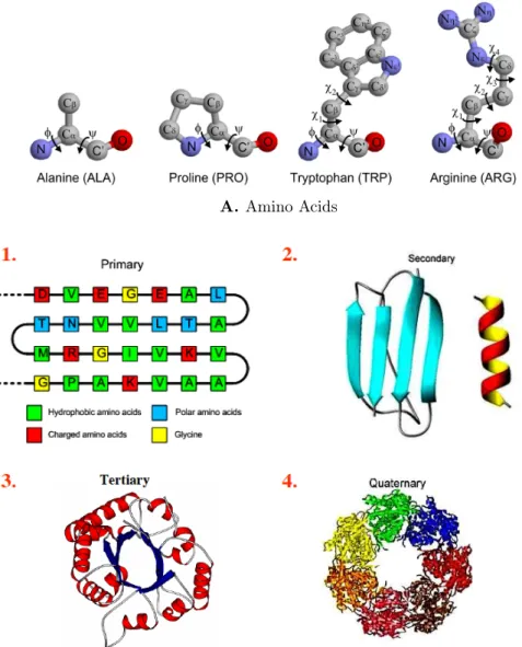
1-2 A) Some examples of amino acids. B) Protein structure is described in a hierarchical manner, ranging from a primary structure to a qua-ternary structure. . . 4

1-3 Schematic of protein threading. A) A protein 3D structure is first reduced to a simplified representation as a graph, with residues as the nodes and edges between residues that are physically close in the 3D structure. This simplified representation is known as the template. B) The target sequence (query) is then “threaded” onto the template to find the best sequence-structure alignment. This is usually formulated as an optimization problem, with both sequence and structure features in the objective function. The dashed lines represent alignment of the residues of the template to residues of the target sequence [95] . . . . 7

1-4 A) A binary PPI complex. Red and blue are two proteins, and the interface residues are highlighted in green. B) A contact map repre-sentation of the complex in a. The entries in the map are color-coded ranging from red (low) to black (10Å). Distances greater than 10Å are not relevant and are indicated by white. . . 10

(14)

1-5 A) Residue composition at the interface in a non-redundant set of protein complexes. B) Residue propensities at the interface in the non-redundant set of protein complexes. “Core” of the protein refers to interior of the protein. Hydrophobic residues have a higher propensity at the core, whereas polar amino acids are enriched at the interfaces and surfaces. Figures taken from [178]. The residues are arranged in increasing order of their hydrophobicity (Kyte-Doolittle scale) from left to right [93]. . . 12

1-6 Schematics of the popular HTP techniques for PPI detection. A) Yeast-2-hybrid method involves fusing the two candidate proteins (X and Y) to a DNA binding domain (DBD) and an activator domain (AD) of a transcriptional factor. Interaction between the proteins results in a functional transcriptional complex, ultimately leading to the expression of the reporter gene [5]. B) In the TAP-MS method, the bait (X) along with its partner proteins are extracted from the cellular contents with the help of a fused tag. The constituents are then separated and identified using MS [140]. C) Protein chips involve immobilizing prey proteins by fixing them on a chip. The bait protein (X) is fused with a fluorescent tag to help visually identify the PPIs [140]. D) In a Lumier assay, the bait protein is fused with a luminescence protein, and the prey is fused with a tag to help in purification. After extraction of the bait-prey complex from cellular contents, the interaction is detected by monitoring the luminescence observed [47]. . . 16

(15)

1-7 A) Interaction between A and B is transferred to A’ and B’ using or-thology assignments [96]. B) Structure-based prediction of the putative interface using homology modeling or threading. The candidate pro-teins are first aligned to a complex template, and the putative interface is inferred from the structure and the alignment. c) One example of a data integration method. Multiple features such as Gene Ontology (GO) annotation similarity, co-expression and co-localization for a pair of query proteins are input into a random forest classifier that makes a prediction. . . 21

2-1 Struct2Net algorithm. The input to the algorithm are two protein sequences. The first stage consists of identifying the best complex template for the two proteins, and alignment of the proteins to the template using DBLRAP (Double RAPTOR) [177, 143]. In stage 2, a set of scores quantifying the quality of the alignment and predicted interface are extracted from the sequence-structure alignment of stage 1 and input into a classifier that predicts the probability of interaction. 28

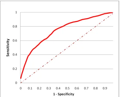
2-2 The prediction algorithm can achieve 60% sensitivity while maintain-ing 75% specificity as measured on the test set. Here, sensitivity = (true positives)/ (true positives + false negatives) and specificity = (true negatives)/ (true negatives + false positives). We constructed a training set and test set of positive and negative examples from yeast and fly, using criteria we have developed to identify high-confidence positive and negative examples of PPIs [142]. After training the logis-tic regression model on the training set, its performance was measured on the test set. . . 32

(16)

3-1 A) Cartoon depicting how iWRAP’s interface threading uses multiple templates to identify the putative interface region for the two query proteins. All the templates belong to the same SCOPPI family. B) Overview of the iWRAP’s interface threading approach for PPI pre-diction [68]. . . 39

3-2 Schematic describing the cross-validation testing of iWRAP on the in-terface database SCOPPI. Sequences of a test complex belonging to the same family as the template, but less than 40% identical to it, are threaded onto the template using an alignment program. The pre-dicted interface (from the threading alignment) is then compared with the actual interface (from the known structure) to compute accuracy. Dashed lines indicate the aligned interface computed using the align-ment program, solid black lines indicate the actual interface mapped from the true structure. . . 44

(17)

3-3 Example of improved contact predictions by iWRAP in within-family cross-validation. PDB 1upc chains A(12-195) and B(375-573) are threaded to the template 1qpbAB. A) The true interface computed from the PDB structure of 1upc has roughly 50 contacts. The interface residues are shown as purple spheres, chain B is shown in red and chain A in blue. B) The template (1qpbAB) used for threading the query se-quences; the interface residues are shown in green. C) The interface residues (yellow spheres) predicted by DBLRAP. DBLRAP fails to align the interface region of one interacting partner due to low sequence homology between the query and template (contact accuracy = 0%). D) Initial interface (yellow spheres) predicted by iWRAP after thread-ing (contact accuracy = 27%). iWRAP uses interface profiles con-structed from a multiple alignment of the interfaces 1mczHG, 1jscAB, 1ozhDC and 1qpbAB; the profiles are then mapped onto the template 1qpbAB. E) Final interface (yellow spheres) predicted by iWRAP after contact map optimization. This step refines the contact map, resulting in contacts closer to the true interface. The final contact map is closer to the true contact map (contact accuracy = 46%). This is obtained by overlaying iWRAP predictions (yellow) on the actual structure of the interface (from A). F) Predicted interface structure obtained by mapping true interface residues from A onto the template structure in B using iWRAP alignments. . . 46

(18)

3-4 Interface alignment and contact validation. Panels A, B, C and D are cross-validation results on within SCOPPI family threading. ∆(contact

accuracy|δ|=2) is the difference in contact accuracies (|δ|=2) between

iWRAP and DBLRAP. A) Contact accuracy improvement of iWRAP relative to DBLRAP as a function of number of true contacts at the interface. B) Contact accuracy improvement of iWRAP relative to DBLRAP as a function of sequence identity at the interface. C) iWRAP consistently achieves lower average interface energies as com-pared to DBLRAP. D) RMSD comparison between iWRAP and DBLRAP-better contact prediction by iWRAP does not affect RMSD of the pre-dicted interface. E) Cross-validation results for interfaces sharing only one SCOP family (seeCross-validation across SCOPPI families). See

Appendix A for calculation of contact accuracies and interface energy. 47

3-5 Results on the yeast genome. Sensitivity vs specificity for iWRAP, Struct2Net and iWRAP+DBLRAP (combined method). In the

com-bined method, DBLRAP threading results are boosted and comcom-bined with iWRAP predictions. AUCs for the three methods are: 0.734 (iWRAP), 0.680 (Struct2Net) and 0.762 (combined). All the differ-ences are statistically significant (P < 10−10, t-test).Here sensitivity

= (true positives)/ (true positives + false negatives) and specificity= (true negatives)/(true negatives + false positives). . . 51

(19)

3-6 iWRAP predicts novel, bona fide interactions. A) Enrichment anal-ysis was carried out to identify high-confidence interactions. Genes filtered by co-localization and significantly enriched compared to the genetic interaction set were validated using the Oncomine and HCPIN databases. Number of genes remaining after each stage are indicated in parantheses. B) The analysis in A reveals a set of high-confidence genes (green) predicted to be interacting with yeast homologs of cancer related genes (purple). Human orthologs of genes for which there is lit-erature providing evidence of implication in cancer have been indicated in parentheses. Genes interacting with only one “cancer” (purple) gene are in the outermost circle, whereas those interacting with more are in the innermost circle. Genes which are not significantly enriched are colored in grey, however, these predicted interactions could also reveal novel biological insights. The figure was created using Cytoscape [136] 56

3-7 Schematic of interface threading and contact optimization. For the example shown in Figure 2, the query proteins are individually aligned to the template (left) using a local alignment to the interface (dashed lines). For scoring this alignment, we use the interface profiles com-puted from the multiple-interface alignments, predicted secondary struc-ture for the query pair and the single-domain threading score of RAP-TOR. Minimizing this alignment score produces an initial contact map, ‘iWRAP initial’, which is further refined using Hadamard product op-timization and quasi-chemical pairwise residue potentials to produce ‘iWRAP final’ (right). . . 58

(20)

4-1 Framework for assessing confidence in a HTP PPI screen. Coev2Net, re-trained on a high-quality PPI network, is able to assign structure-based confidence scores for HTP PPI networks. Each node represents a protein and each edge the putative interaction between the two pro-teins. The thickness of an edge describes structure-based confidences of putative PPIs. . . 70

4-2 Flowchart of Coev2Net. Left: MCMC sampling to generate synthetic homologous sequences for each complex template. Right: 1) For given query protein pairs, the best template (from the structural library) is identified by user-defined protein threading; 2) structural and sequence features are extracted from the interfacial alignment and residue cor-relations scored w.r.t. the profile PGM; and 3) a classifier gives the probability of interaction for the query protein pair. . . 72

(21)

4-3 A) Overlap of the Vinayagam (blue) and Bandyopadhyay (red) datasets (left). The study by Bandyopadhyay et al. reveals 2269 interactions with 641 “core” interactions supported by multiple lines of evidence, whereas the Vinayagam dataset has 2626 interactions connecting 1126 proteins. Differences in the two experimental techniques are high-lighted by the fact that only 170 nodes and 6 interactions overlap in the two sets. B) Coev2Net predicted high-confidence network is shown on the right. Edge colors correspond to the dataset they come from. MAPK6 has the highest degree, and its label is shown explicitly. C) Comparisons of performance on MAPK network for Coev2Net and pre-vious Struct2Net (iWRAP+DBLRAP) [143, 142, 68] in terms of sensi-tivity and specificity. Coev2Net performs much better than Struct2Net on this dataset (core network of Bandyopadhyay et al.), and its perfor-mance is robust with respect to the randomness in MCMC sampling. The classifier (Fig 4-2) is trained and tested via 5-fold cross-validation on the core network. The MCMC procedure is repeated 5 times to assess robustness of the predictions. ’Baseline’ method represents a logistic regression classifier with just the alignment features and no PPI (either Coev2Net or Struct2Net) features. D) Experimental vali-dation of predicted high-confidence interactions using LUMIER assay. Typically a fold increase of 1.5 is considered as a true positive. . . 75

(22)

4-4 Predicted interfaces are enriched for SNPs in the Coev2Net predicted high-confidence MAPK network. A) Relative distribution of PolyPhen annotated mutations at the interface and non-interface. B) SNP (PolyPhen annotated) prevalence at the interface and non-interface. C) Somatic mutations characterized as “missense” preferentially fall on the inter-face (bottom). The white circles represent corresponding means. Error bars represent the 75%-25% data range. . . 77

4-5 A) Predicted interface for the interaction between BRAF (light blue) and PAK2 (red surface). Cancer associated mutations that are anno-tated are shown in magenta. In dark blue we indicate mutations that are predicted to be associated with cancer but with no current anno-tations. Rest of the template structure is shown in gray. Mutations were taken from MoKCa database [129]. B) Predicted interface for the interaction between MAPK6 (yellow) and YWHAZ (cyan). Phospho-rylation sites on the proteins are indicated in red (S189 for MAPK6 and S184 for YWHAZ). The template used for the prediction was 1F5Q (chains A and B). . . 80

5-1 Methods introduced in this thesis. DBLRAP predicts the entire struc-ture of the putative complex from the query sequences. iWRAP uses interface profiles that characterize biophysical properties of protein in-terfaces to predict just the interface residues. Coev2Net scores the predicted interface using a probabilistic graphical model that encodes long-distance correlations (i.e compatibilities) at the interface. The interface in this case can be obtained from any threading/alignment method. . . 89

(23)

A-1 Example of an interface template. A) An example of a multiple inter-face alignment from CMAPi (only one core is shown). The upper case letters represent the contacting residues in the interface, profiles con-structed from residues highligted in red are shown in B. B) Interface template encoding the consensus residues, consensus secondary struc-ture class and average solvent accessibility at the highlighted (in red) alignment positions inA. “X” represents the gap state in the alignment. 95

A-2 Precision vs recall for theS.cerevisiaepredictions. Here, precision=true

positives/(true positives + false positives) and recall = true positives/(true positives + false negatives). . . 99 B-1 Singleton (A) and Pairwise (B) probabilities at the interface calculated

from a non-redundant set of complexes in [98] . . . 105 B-2 Cross-validation results on SCOPPI. (left) Results on SCOPPI

fami-lies having 3 or more complexes. (right) Results on SCOPPI famifami-lies having only 2 complexes (1 training and 1 test) . . . 107

(24)

(25)

List of Tables

2.1 Number of interactions in Biogrid [151] for common eukaryotic organisms. 25 3.1 Comparison of iWRAP with other sequence and structure based

tech-niques on cross validation tests in SCOPPI. The numbers indicate the alignment accuracies at the interface, with the true alignments taken as the ones given by CMAPi [124] . . . 42 3.2 The most frequent templates used by iWRAP for threading sequences

involved in high-confidence interactions in Biogrid unique to iWRAP. Column 2 gives the total number of pairs threaded using the template, column 3 gives the number of pairs in the test set and column 4 gives the average predicted probability of interactions in the test set. A template id ‘1v55B2-1v55A2’ represents the interface formed by SCOP domains in chain B and chain A in the PDB complex ‘1v55’. . . 54 4.1 Comparison of overlaps achieved by Braun et. al. and our method

when some of the initial Y2H interaction pairs are re-tested using LU-MIER assay. . . 74

(26)

(27)

Abbreviations

AUC Area under receiver operator characteristic curve (ROC) ASA Accessible surface area (by solvent)

FDR False discovery rate GO Gene Ontology

HMM Hidden Markov model HTP High-throughput

LUMIER Luminescence-based mammalian interactome mapping MSA Multiple sequence alignment

mRNA Messenger ribonucleic acid NR Non-redundant

PDB Protein data bank

PPI Protein-protein interaction

ROC Receiver operator characteristic curve SNP Single nucleotide polymorphism TAP Tandem affinity purification Y2H Yeast two-hybrid

(28)

(29)

Glossary

Interactome The whole set of protein-protein interactions in an organism.

AlignmentA one to one mapping of characters (amino acids or nucleotides) between

two protein (or DNA) sequences. The mapping respects the ordering of the characters in the individual sequences. If a character cannot be mapped, it is usually aligned to a “gap”. A multiple sequence (or structure) alignment (MSA) is an alignment between multiple sequences (or structures). MSA is usually visualized as a matrix with the number of rows equal to the number of sequences that are aligned and the number of columns equal to the alignment length.

Sequence profileThe set of distributions (or frequencies) describing the composition

of the columns of a multiple sequence alignment (MSA).

Genotype The genetic makeup of a cell (i.e. the specific genetic sequence), usually

with reference to a particular trait under consideration.

Phenotype The composite of an organism’s observable traits and characteristics. Homologs Two protein (or DNA) sequences are said to be homologous if they share

an ancestor. Homology is usually determined by sequence similarity between the two proteins.

Orthologs Two homologous proteins are orthologous if they are present in different

species and resulted from a speciation event.

Non-redundantIf two protein sequences have less than a threshold sequence

(30)

imply that each sequence in the database is different from every other sequence in the database with respect to the threshold sequence similarity.

Complex Complex refers to a group of proteins involved in an interaction. In

struc-tural bioinformatics and in this thesis, a complex refers to the structure of a binary protein interaction.

Phylogenetic treeA tree showing the evolutionary relationships (inferred) between

protein sequences (or DNA sequences). It is usually based on sequence similarities between the sequences.

(31)

Chapter 1 Introduction

A genome of an organism encodes for tens of thousands of proteins (proteome) that make specific interactions with other proteins and bio-molecules. Systematically map-ping these interactions (the interactome) is a major challenge in post-genomic biol-ogy. Elucidation of the interactome of a cell is an essential first step in understanding protein function and cellular behavior. Sustained focus on reconstructing the inter-actomes of various model organisms in recent years has resulted in a wealth of infor-mation. Indeed, in this new era of high-throughput (HTP) technologies, molecular biology is dominated by studies on pathways, complexes or even an entire organism. A mechanistic understanding of how molecules interact comes only from three dimensional (3D) structures, as they provide a high resolution picture of the bind-ing. Such an understanding allows us to design experiments that perturb systems in an intelligent way. Consequently, knowledge of these atomic details provides us with a rational way of developing therapies by repairing and/or inhibiting interac-tions [5]. Despite their invaluable contribuinterac-tions, atomic details of interacinterac-tions are beyond the scope of current HTP protein-protein interaction (PPI) detection tech-niques. Structural-genomics initiatives and advancements in structural biology are steps in the right direction, but are lagging behind other technologies for PPI

(32)

de-tection. Moreover, the sheer number of interactions to test (e.g. 50 million possible

pairs for an organism with 10000 proteins) makes it an insurmountable task for any

one experimental technique alone.

The thesis aims to bridge this gap between new-era HTP systems biology and traditional computational molecular biology to give a high-resolution understanding of the interactome. By developing protein-protein interaction (PPI) prediction tech-niques based on atomic details of protein 3D structures, the thesis provides a deeper understanding of structure-function relationships in biological systems. Moreover, the methods developed in this thesis help overcome the limited and biased sampling of experimentally verified interactions, ultimately leading to a complete high-quality mapping of the interactome.

The rest of the chapter is structured as follows. First, in section 1.1, basics of protein structure, structure determination and computational aspects of protein structure relevant to the thesis are introduced. Then, in section 1.2, aspects of protein-protein interactions (PPI), including experimental and computational methods for PPI prediction are discussed. Finally, I explain how understanding the structure-function relationship in the context of PPIs will help design better therapies for human diseases.

1.1 Proteins

The central dogma of molecular biology states that genes in the DNA are transcribed to mRNA, which are then translated to a sequence of amino acids called proteins (Figure 1-1). There are 20 different types of amino acids, each differing only in their side-chains. This difference leads to differences in the physicochemical properties of the amino-acids, ultimately influencing the function of the protein. Each amino acid, also called a residue, has a bonded sequence of three atoms, a nitrogen and two

(33)

Figure 1-1: Central dogma of molecular biology. Fromhttp://www.lhsc.on.ca

carbons. The same triplet of atoms from each residue of a protein are concatenated together via a peptide bond to form the backbone of the protein. Each residue has a side-chain containing 0 to 10 heavy atoms branching out of the middle carbon atom (Cα). Some examples of amino acids (residues) can be seen in Figure 1-2 [21].

In its most basic form, a protein can be thought of as a linear copolymer formed by the concatenation of amino acids (primary structure). More generally, protein structure is described in a hierarchical manner: ranging from a “primary” structure to a “quaternary” structure. Under physiological conditions, the primary structure folds to a unique, compact and relatively stable 3-D structure, which determines its specific biological function. The sequence of the protein is believed to completely encode its folded structure, which arguably corresponds to the minimum free energy of the molecule. Furthermore, different regions of the sequence form one of two local regular structures - alpha helix (α) and beta sheets (β). These locally compact

structures are referred to as secondary structure. The tertiary structure is obtained by packing such structural elements into one or more compact globular units called domains. In many proteins several polypeptide chains forming different domains are brought together to form a quaternary structure (see Figure 1-2) [21].

(34)

!

A. Amino Acids

!

B.Hierarchy in protein structure

Figure 1-2: A) Some examples of amino acids. B) Protein structure is described in a hier-archical manner, ranging from a primary structure to a quaternary structure.

(35)

1.1.1 Protein structure determination

Protein function is determined by its structure. As a result, a lot of effort has been devoted to determining the 3D structure of proteins [18]. The most popular techniques for structure determination are X-ray crystallography and NMR spectroscopy [42]. Close to 85% of protein structures deposited in the Protein Data Bank (PDB) are determined by X-ray crystallography [14]. Although these techniques have given us invaluable information about protein structure and function, they are laborious and time consuming. For example, it is not uncommon to take on the order of 6 months to a year to solve a protein’s structure using X-ray crystallography [21, 42, 67]. Furthermore, not all proteins are amenable to crystallography or NMR spectroscopy (e.g transmembrane proteins) [42].

Since protein structure is encoded in its sequence, it should be possible to com-putationally predict the 3D structure of a protein just from its sequence, using laws of physics and chemistry. To overcome limitations of structure determination tech-niques and to better understand protein folding, structure prediction has remained one of the most active areas in computational molecular biology [18]. There are three broad categories into which the various structure prediction methods are divided: 1) homology modeling, 2) protein threading and 3) ab initiofolding. In homology

mod-eling, the structure of a protein is predicted by identifying a homologous protein in the PDB. It exploits the common rule of thumb that sequences that are similar, fold in a similar way. Therefore, given the target sequence (for which the structure is to be determined), a database of solved structures is searched for similar sequences. The predicted structure is then built using large fragments of these related structures. As more and more structures are solved, homology modeling will become increasingly accurate as there is a greater chance of finding a similar sequence in the database. Depending on sequence similarity, it is sometimes possible to get structures as good as a medium resolution X-ray crystallographic structure [183]. But usually, as the

(36)

se-quence similarity between a target and the candidate structure goes down, it becomes an incorrect representation of the actual structure of the target sequence.

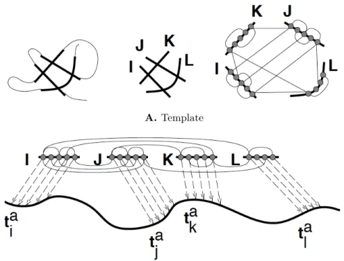
For sequences that do not have any clear homologs in the PDB, protein threading is the method of choice for structure prediction. Compared to homology modeling, which considers only the sequence similarity between the target and a candidate struc-ture, protein threading makes use of structural information encoded in the candidate structure to improve prediction accuracy. The main components of a threading ap-proach are a template (a simplified representation of the protein 3D structure) and a scoring function to evaluate an alignment. The goal of a threading algorithm is to find the best alignment of the target sequence to the template structure in the space of all possible alignments. Figure 1-3 gives a schematic of the components of a threading approach. First, a template is constructed from the 3D structure of the protein. Then, alignments are scored using a scoring function that evaluates the compatibility of the aligned target residue in the structural environment of the cor-responding aligned template residue. In Figure 1-3b, regions of the target sequence aligned to corresponding fragments in the template are indicated by the lettersta _and

the alignments are represented as dashed arrows. Computing the optimal alignment (i.e. best alignment score) is formulated as a combinatorial optimization problem, and a variety of mathematical techniques are used to solve it [183]. Different thread-ing programs use different scorthread-ing functions. All of them usually include secondary structure, solvent accessibility and pair-wise interactions in scoring an alignment. One of the best threading programs used in structural bioinformatics is RAPTOR [177]. RAPTOR formulates the alignment problem as an integer linear programming problem (ILP), and uses a branch and bound technique to efficiently solve the ILP [177]. The methods developed in the thesis use this formulation of RAPTOR for structure prediction.

(37)

A.Template

B. Sequence to structure alignment

Figure 1-3: Schematic of protein threading. A) A protein 3D structure is first reduced to a simplified representation as a graph, with residues as the nodes and edges between residues that are physically close in the 3D structure. This simplified representation is known as the template. B) The target sequence (query) is then “threaded” onto the template to find the best sequence-structure alignment. This is usually formulated as an optimization problem, with both sequence and struc-ture feastruc-tures in the objective function. The dashed lines represent alignment of the residues of the template to residues of the target sequence [95]

complete structure from the PDB. The main difficulty arises because conformational search space increases dramatically with respect to protein size. The optimization problem is usually non-convex and requires techniques based on Monte Carlo methods and genetic algorithms to tackle the inherent complexity [183].

1.2 Protein-protein interactions

Proteins interact with other proteins and molecules to perform their function. In this thesis, we are mainly concerned with understanding protein-protein interactions (PPIs) and using that knowledge to predict PPIs. Our knowledge about the rules

(38)

of association of protein molecules comes mainly from studying structures of protein complexes. We will look at methods to characterize structural features of interfaces, their chemical composition and their evolutionary histories. All these aspects of PPIs are relevant for subsequent chapters in the thesis.

1.2.1 Types of PPIs

Interactions between two proteins (binary PPIs) are usually divided based on the type of proteins that interact, stability of the proteins and duration of interaction. Inter-action between two identical protein chains is called a homo-oligomeric complex (or homo-dimer or homomer), whereas interaction between different proteins is called a hetero-oligomeric complex (or heteromer). Based on stability, interactions are divided as obligate and non-obligate complexes [112]. Proteins forming obligate complexes do not form stable functional structures on their own, whereas proteins in non-obligate complexes can form stable structures. Many heteromers are non-obligate, while ho-momers are often obligate [112, 78]. In terms of duration, interactions are divided as transient or permanent. Transient interactions last for seconds or less, and typ-ically regulate critical cellular processes by protein phosphorylation or acetylation. Permanent (stable) interactions have a typical half-life of 12 minutes to 19 hours and include some of the biggest structures in a cell such as core RNA polymerase, DNA replication complexes, etc [118]. Permanent complexes can be readily detected by common experimental techniques such as co-purification and yeast-2-hybrid (Y2H). Transient interactions are more difficult to detect, requiring some prior knowledge of the two interacting proteins and the conditions under which they interact [118, 131].

1.2.2 Structural features

The interface between two interacting proteins in a complex can be defined in a variety of ways. The most popular and simplistic definition is that of a minimum distance –

(39)

if the distance between any two heavy atoms of two residues on either protein is less than 5Å, the two residues are said to be interacting and part of the interface. Another characterization of interface residues is in terms of accessible solvent area (ASA). In protein complexes, it has been observed that 20-45% of the interface residues have very low ASA (close to zero), and they tend to be hydrophobic [73]. Sometimes these residues are also referred to as the “interface core”, with the “interface rim” consisting of residues that are less than 10Åapart in the 3D structure and having non-zero ASAs. Interfaces can also be described to reflect shape complementarity between the interacting proteins, cavities on the surface of the two proteins and atomic packing. Typically, such representations are based on embedding a 3D grid on top of the structure and measuring the volumes occupied by each atom. More generally, techniques such as voronoi diagrams allow for a precise estimation of the atomic packing [73, 89].

Another popular method of representing an interface is that of a contact map. A contact map is a 2D representation of the 3D interface, with the aim of representing only residue-level information. A contact map is a matrix of dimension mxn, where m and n are the lengths of the two proteins. An entry ij in the contact map is

the minimum distance between any two heavy atoms in residue i in one protein and

residue j in the other. If the minimum distance is greater than 10, a zero is used

instead. For a cleaner visualization and tractable computations, only rows/columns that have at least one non-zero entry are retained, the rest are discarded (see Fig-ure 1-4). As can be seen, such a representation allows one to design fast search and alignment algorithms without having to deal with the more complicated 3D topology.

1.2.3 Physico-chemical features

The physico-chemical features of an interface depend on the relative abundance of different amino acids at the interface. Amino acids are usually described as

(40)

non-A. Protein-protein complex B. Contact Map

Figure 1-4: A) A binary PPI complex. Red and blue are two proteins, and the interface residues are highlighted in green. B) A contact map representation of the com-plex in a. The entries in the map are color-coded ranging from red (low) to black (10Å). Distances greater than 10Å are not relevant and are indicated by white.

(41)

polar/polar/charged, or in a more coarse-grained model as hydrophobic/hydrophilic. The composition of an interface is usually computed by counting interface atoms or residues, or by weighting their numbers by their buried surface area (BSA). The advantage of area-based composition is that it accounts for the amino acid size as well. Quantitatively, interface propensity is calculated as:

pi =log( fi fo i

) (1.1)

wherepi is the propensity of amino acid of type i at the interface,fi is the number

or area fraction of type i at the interface, and fo

i is the corresponding number in a

reference set (can be the whole protein, or its interior, or surface). Interpreting pi is

straightforward: ifpi> 0, then the interface is enriched for atoms or residues of type i

compared to the reference set, andpi < 0 implies that the interface is depleted of type

i. Figure 1-5 shows the composition and propensities calculated from a non-redundant set of protein complexes [178].

Hydrophobicity plays an important role at protein surfaces and interface. Amino acids containing groups with ‘O’ and ‘N’ in their side chains are polar and hydrophilic, the rest are non-polar and hydrophobic. Hydrophobic patches enriched for such residues are frequently found at protein interfaces, indicating that their contribution to PPIs is significant. It has been argued that capping motifs which bury otherwise-exposed hydrophobic patches have specifically evolved in certain proteins to prevent aggregation [24]. The extent of the hydrophobic contribution depends on the type of interaction and the driving force (i.e long-range electrostatics or short-range desolva-tion effects). For homo-dimers/obligate complexes, the monomer (protein) molecules do not exist individually and hence their interfaces tend to be always buried (from the solvent). Therefore, such interfaces can have large hydrophobic patches. Interactions in which each participating protein exists as a functional unit by itself cannot admit large hydrophobic patches on its surface as it would be energetically unfavorable [78].

(42)

A. Interface composition

B. Interface propensities

Figure 1-5: A) Residue composition at the interface in a non-redundant set of protein com-plexes. B) Residue propensities at the interface in the non-redundant set of protein complexes. “Core” of the protein refers to interior of the protein. Hy-drophobic residues have a higher propensity at the core, whereas polar amino acids are enriched at the interfaces and surfaces. Figures taken from [178]. The residues are arranged in increasing order of their hydrophobicity (Kyte-Doolittle scale) from left to right [93].

(43)

Electrostatics also plays an important role in PPIs, as can be seen from Figure 1-5. Enrichment of polar amino acids indicates that protein interfaces tend to be more similar to protein surfaces than to protein interiors. One hypothesis for explaining this apparent anomaly is that desolvation effects are partially compensated in inter-faces through the formation of networks of ion-pairs and hydrogen bonds, which are positioned so as to interact favorably with one another. Electrostatics is also known to play a significant role in the rate of protein-protein association [137]. Computa-tionally, accounting for electrostatics requires elaborate calculations that are highly sensitive to the solvent model and local structural environment. The representation of electrostatics is not accurate enough yet, although it has resulted in a few excellent models for protein-protein complexes [20, 134]. Such calculations are usually compu-tationally intensive and left for later stages of structure prediction, with earlier steps relying on statistical (knowledge) potentials [73].

1.2.4 Evolutionary features

As we have seen in the previous two sections, in order for two proteins to interact, there has to be structural as well as chemical compatibility at the interface. One can then argue that nature will try to maintain this compatibility over the course of evolution of the species. Indeed, evolutionary conservation has been observed at three levels in PPIs: 1) interface residues are conserved across orthologs in different species, 2) co-evolution of residues at the interface of the interacting proteins (correlated mutations), and 3) similarity of phylogenetic trees (evolutionary histories) for the two proteins [83, 79, 164, 72, 80]. Notice that the first two observations are at a residue-level and hence require multiple interacting proteins from different species to give any meaningful statistics. This kind of information is usually not available for all possible protein pairs, and hence these insights have generally not been used for prediction purposes till now. We will however develop techniques that overcome

(44)

this difficulty. Compared to the first two, similarity between phylogenetic trees is an indirect evidence for interaction. Correlation between phylogenetic trees could arise due to a variety of reasons not necessarily related to PPIs. It does not give us any residue-level insight into the interface compatibility of the two proteins [163, 164].

1.3 Experimental methods for PPI detection

1.3.1 Low throughput screens

Low throughput (LTP) experimental techniques include affinity chromatography, affinity precipitation, dosage lethality, biochemical assays, synthetic lethality and structure [151]. Interactions detected by these experiments are usually reliable and used as gold-standard [35, 168]. However, it is difficult to curate interactions detected by LTP experiments since one has to manually go though the publication to extract the interacting pairs. Text mining is still in its infancy, and leads to numerous false positives and negatives [111]. Moreover, the number of interactions that need to be identified to map the entire interactome is too large to be done using LTP screens alone.

1.3.2 High throughput screens

High throughput (HTP) screens have provided the bulk of the interactions that we know today [151, 133]. These methods are called HTP because thousands of pairwise interactions can be tested simultaneously. HTP methods include yeast-2-hybrid (Y2H) [54, 130, 162, 155, 181, 141], mass spectrometry based methods [88, 64, 31, 48, 58], protein chips [176, 185, 186] and LUMIER assays [12].

(45)

Yeast-2-hybrid method

The two-hybrid system is one of the most widely used HTP screen for PPI detection. It is based on the observation that gene transcription requires the binding of two domains of a transcriptional activating protein [51]. These domains are called DNA binding domain and activator domain (Figure 1-6). The candidate proteins are fused to one of the two domains. If the two candidate proteins interact, then the DNA binding domain and activator domain are close enough to interact and result in a functional transcription complex. This activates expression of the reporter gene, leading to an observable change in phenotype (e.g. fluorescence).

Mass spectrometry based methods

Mass spectrometry (MS) is an analytical technique to identify the chemical com-position of proteins and peptides. For PPI detection, two types of MS-based HTP techniques are popular - tandem affinity purification (TAP-MS) and protein complex identification (HMS-PCI) [19, 58, 66]. In these techniques, the protein whose interact-ing partners are sought is called the bait and its interactinteract-ing partners are called prey. Both the techniques first fuse short tags to the bait so that they can be extracted from a mixture of cellular contents (Figure 1-6). If a bait is part of a complex, then the complex is first extracted and its constituents are separated by gel electrophoresis and identified by MS.

Protein chips

Protein chips (or microarrays) involve thousands of proteins immobilized on the sur-face of a microscope slide. Labelled target proteins are then added to the chip and may bind to some of the proteins on the chip. Unbound proteins are washed away and the bound ones are detected using a fluorescent dye [185, 186].

(46)

A. Yeast-2-hybrid B.TAP

C. Protein array D. Lumier

Figure 1-6: Schematics of the popular HTP techniques for PPI detection. A) Yeast-2-hybrid method involves fusing the two candidate proteins (X and Y) to a DNA binding domain (DBD) and an activator domain (AD) of a transcriptional factor. In-teraction between the proteins results in a functional transcriptional complex, ultimately leading to the expression of the reporter gene [5]. B) In the TAP-MS method, the bait (X) along with its partner proteins are extracted from the cel-lular contents with the help of a fused tag. The constituents are then separated and identified using MS [140]. C) Protein chips involve immobilizing prey pro-teins by fixing them on a chip. The bait protein (X) is fused with a fluorescent tag to help visually identify the PPIs [140]. D) In a Lumier assay, the bait protein is fused with a luminescence protein, and the prey is fused with a tag to help in purification. After extraction of the bait-prey complex from cellular contents, the interaction is detected by monitoring the luminescence observed [47].

(47)

Lumier assay

Luminescence based mammalian interactome mapping (LUMIER) is a new technique developed to detect even transient interactions in signaling networks [12]. In a Lumier assay, a luciferase-tagged bait protein is screened against a series of flag-tagged prey proteins; an antibody against flag is used to affinity-purify the prey, and the prey-associated luminescence on exposure to an appropriate luciferin substrate is monitored to detect interaction [47]. The technique is known to be more sensitive than previous approaches, and comparatively easier to quantify dynamic shifts in PPI networks [47].

1.3.3 Limitations of experimental techniques

HTP screens look very promising as they identify thousands of interactions, but they suffer from high false-positive and false-negative rates [65, 16, 165, 148]. Estimates on the false discovery rates (FDR) 1 in HTP techniques are still debated as there is

no gold-standard for negative data (i.e. proteins that do not interact) to evaluate against. Initial estimates computed from re-testing interactions detected by HTP experiments obtained FDRs in the range 20-40% [130, 155]. More recently, with improvements in experimental protocols, HTP studies were able to achieve FDRs between 0 to 11% [22]. Although these values seem reasonable, the more serious issue is with sensitivity of these assays. Braun et al. evaluated 5 HTP methods and obtained sensitivities of 21 to 36% [22]. Combining the methods resulted in a sensitivity of around 59% [22]. The main strategies for improving the FDR and sensitivity of HTP methods are by repeating screens, using several HTP screens or combining HTP and computational approaches for PPI prediction [181, 43]. However, conducting repeated screens or using multiple HTP screens is time-consuming and not cost-effective [135]. For example, some estimates put the time required for completing the Drosophilia melanogaster interactome at 1700 person-years, using the current

(48)

experimental protocols [135]. Using a ranked list of interactions to test reduces this estimate considerably to 385 person-years [135]. Moreover, it has been argued that limited overlaps of interactions identified using different HTP techniques highlight the biases of those experiments rather than identify true/false positives [166, 165]. More importantly, non-physiological conditions in most experimental techniques limit our ability to translate detected PPIs into in vivo hypotheses.

1.4 Computational methods for PPI prediction

Limitations in experimental techniques combined with the sheer number of inter-actions to verify has provided much impetus to the development of complementary computational methods for PPI prediction. These methods usually use a variety of machine learning, statistical and graph-theory based approaches. Computational methods for PPI prediction can be roughly divided into three broad categories - in-direct methods, in-direct methods and methods based on data-integration.

1.4.1 Indirect methods

Indirect methods for PPI prediction are methods that try to infer physical interaction between two proteins based on evidence for their functional association. One of the popular methods for detecting functional association is by correlation of gene expression profiles (co-expression) [96]. The idea here is that genes showing a high correlation in their expression patterns under different conditions are more likely to physically interact than random pairs. On a genomic level, functional association is usually detected by conservation of gene neighborhood, similar pattern of presence or absence across multiple genomes or gene fusion [96]. The intuition behind such approaches is that if the genes are functionally related, they will tend to be inherited as a unit since the loss of one gene would disrupt the function they are involved

(49)

in. However, such methods are always used as additional sources of evidence since functional association need not always imply direct physical interaction [5, 96].

1.4.2 Direct methods

Direct methods for PPI prediction usually use the primary sequence or tertiary struc-ture in a direct way to infer PPIs. Methods that use protein sequence generally con-sider the physicochemical properties of the constituent residues and/or frequencies of residue combinations to quantitatively predict PPIs [17, 63, 105, 120, 180]. Most techniques map the protein sequences onto a multi-dimensional feature space, and use machine learning based classification algorithms such as support vector machines, lo-gistic regression, neural networks to quantitatively predict PPIs. The classifiers are usually trained on a small set of high-confidence interactions and evaluated on a separate dataset (i.e. cross-validation) [17, 63, 105, 120, 180].

Another popular method for PPI prediction utilizing protein features is based on the “guilt-by-association” principle. In this method, protein pairs similar to known interacting pairs are predicted to interact. The “association” could be based on se-quence similarity or other properties and annotations [96]. Such associations based on sequence similarity are called “interologs” (Figure 1-7). Predictions made using this approach quickly break down as the sequence similarity between the query and known interactors decreases.

Structure-based approaches are becoming increasingly popular as the number of structures deposited in the PDB is rapidly increasing. In the past 4 years the number of complexes in SCOPPI, a database of protein interfaces, has grown by 60% [173]. For proteins whose structures are not known, homology models or threading based models are typically used to first identify the putative interface. Predictions are then made by evaluating the quality of the interface using a variety of different scoring functions [3, 56, 103, 143, 123, 7]. As shown in Figure 1-7 , such methods proceed

(50)

by first identifying a suitable template for the proteins of interest by scanning the structural database. Optimal sequence-structure alignment then gives the predicted interface, which can be evaluated using either statistical potentials or physics-based potentials for interaction suitability. For proteins that have a solved structure, the challenge is to predict the structure of the bound complex, and evaluate its energy to predict if the two proteins interact. These methods are termed as “docking” methods, with a lot of popular methods available to the community [41, 146, 174, 171].

1.4.3 Data integration methods

Different experimental and computational methods have their own biases, strengths and weaknesses. In general, it is natural to expect an interaction to be true if multiple observations or predictions support it. The data integration methods exploit this intuition by making a prediction based on other predictions or a number of different features. The key challenge here is to integrate different sources of information in an intelligent way by taking into account their individual accuracies. There are many different methods to do this - Fisher’s, Bayesian, logistic regression, random forests, etc [96]. One example of such a method, that integrates co-expression, co-localization and functional similarity using a random forest classifier is shown in Figure 1-7 [143]. Predictions from many of these approaches have been aggregated into a number of databases/web-services offering predicted PPIs. The STRING database [76] com-bines experimental datasets (e.g. BioGRID [151]) with computational predictions based on co-expression, interologs, and text-mining, etc. The entries in this database correspond to functional interactions, and may not always be directly interpretable as PPIs. Another database, IntAct [85], focuses more on inferring interactions from expert curation of data from the literature. Other public services include DOMINO [29], InterDom [109], and I2D [23]. However, all of these databases suffer from a com-mon selection bias: often, the proteins that have been selected for PPI experiments

(51)

A.Interologs Template (complex) Query Predicted interface B. Homology modeling/Threading

GO

Co-expression Co-_localization

Random forest

classifier

True/False

C. Data Integration

Figure 1-7: A) Interaction between A and B is transferred to A’ and B’ using orthology assignments [96]. B) Structure-based prediction of the putative interface using homology modeling or threading. The candidate proteins are first aligned to a complex template, and the putative interface is inferred from the structure and the alignment. c) One example of a data integration method. Multiple features such as Gene Ontology (GO) annotation similarity, co-expression and co-localization for a pair of query proteins are input into a random forest classifier that makes a prediction.

(52)

are usually genes/proteins that have received some attention before and, as such, are also more likely to have functional genomic data.

1.5 Medical impact

Whole genome sequencing and cancer sequencing projects have given us a lot of bio-logical insights into what genes and mutations are associated with diseases. However, this insight has very rarely led to the development of any new therapy to treat such diseases [170]. One main reason for this lack of translational breakthrough has been the difficulty in unraveling the complex genotype-to-phenotype relationships among diseases and their associated genes. Knowledge of PPIs and genome-scale interac-tome has enabled us to tackle this problem like never before, but there is still a long way to go. To gain a complete understanding of biology, it is not enough to know that two proteins interact; it is imperative that we know why and how they interact. This knowledge will enable us to repair disrupted interactions or inhibit aberrant interactions that are often common in many diseases. By doing so, we can design therapies that attack the source of the problem, rather than just treat the symptoms. The methods developed in this thesis not only enable researchers to know whether two proteins interact, they also give insights into why and how they interact. The advantage of this is that experiments can be carried out by mutating the predicted interface residues to further gain an understanding of interaction specificity. There is no doubt that such knowledge will become the basis for designing more efficient drugs and developing new drugs against diseases for which we don’t have any ther-apies. As an example, Pertuzumab, a drug developed by Genentech is designed to inhibit interactions of ERBB3 with other proteins by binding to the same interface, thereby preventing cell division and tumor growth [84].

(53)

1.6 Organization of the thesis

The rest of the thesis is organized as follows: in chapter 2 we take a detailed look at the structure-based PPI prediction methods, which will set the stage for the methods developed in this thesis. In chapter 3, I will introduce a novel algorithm for structure-based PPI prediction that predicts interfaces and PPIs better than previous methods. In chapter 4, we will look at another PPI prediction method that utilizes evolutionary insights to overcome some of the limitations of the previous approaches.

(54)

(55)

Chapter 2 Struct2Net: structure-based approach

to PPI prediction

2.1 Background

The paucity of interactome coverage (Table 2.1) and errors associated with HTP techniques has motivated significant research interest in methods for supplement-ing experimentally determined PPI data with interactions inferred or predicted from other sources. A wide variety of methods have been proposed including the use of “interologs”, functional genomic data such as gene expression, cellular localization and GO annotation (see section 1.4, Figure 1-7).

Organism Number of interactions % of proteins with at least 1 interaction

Mouse 7794 15

Human 65846 57

Fly 24375 46

Yeast 69728 99

Worm 4692 15

Table 2.1: Number of interactions in Biogrid [151] for common eukaryotic organisms.

(56)

proposed. Aloy and Russell suggested the use of structure-based approaches to pre-dicting PPIs [3]. They have described InterPreTS, a web-server to predict PPIs for a given protein, using a homology modeling approach [4]. Lu, Lu and Skolnick con-structed statistical potential functions to evaluate potential PPIs [102] and later de-scribed MultiProspector, a structure-based prediction algorithm [103]. More recently, Fukuhara and Kawabata have described HOMCOS [57] a web-server that performs a similar task, again by homology modeling. Tuncbag et al. have described a method that utilizes evolutionary constraints at the interfaces along with homology model-ing to predict PPIs [159]. MODBase is a database of homology models for protein complexes that have high sequence similarity to known structures [119]. ADAN is a specialized database for prediction of PPIs mediated by linear motifs and utilizes position-specific matrices to assess putative interactions [49]. Other sequence-based methods utilize genetic information and multiple sequence alignments to predict spe-cific protein-protein interactions [163, 164, 25, 138]. There have been methods to predict PPIs based on co-occurrence of sequence domains in the candidate proteins [169]. Other researchers have aimed to understand these domains from a structural perspective. Prieto and Las Rivas [121] have reviewed publicly available databases that facilitate analysis of domain-based PPIs: 3did [154], SNAPPI-DB [75], iPfam [52], PIBASE [37] and PSIBase [61]. While Struct2Net approach has some paral-lels with these approaches, the goal is significantly different. The domain-interaction databases are essentially repositories of known structural data, analyzed specifically from a PPI perspective. Prediction— which is the core goal— is usually beyond the scope of these approaches.

In this chapter, I describe Struct2Net (Structure-to-Network), a structure-based method for predicting protein-protein interactions. Struct2Net predicts interactions by threading each pair of protein sequences onto potential structures in the Protein Data Bank (PDB). Struct2Net provides PPI predictions that are independent of all

(57)

the non-structure-based approaches and may thus be combined with any of them. Another key advantage of Struct2Net is that, apart from the PDB data, the predic-tion algorithm only requires protein sequence data as input. It can thus be applied to proteins for which no functional data is available provided there is a suitable PDB structural template available. Struct2Net offers a significant advantage over other ho-mology modeling approaches. Successful use of hoho-mology modeling requires relatively high sequence similarity between the query and template protein-pairs. In contrast, a threading-based approach widens the range of proteins for which predictions can be made. The use of threading also offers an improved performance: Fukuhara and Kawabata reported that HOMCOS achieves a recall 1 _{of 80% with a precision} 2 _of

about 10%; in comparison, Struct2Net achieves a recall of 80% with a precision of 30% .

2.2 Methods overview

The Struct2Net method proceeds in two stages: 1) identification of the putative interface and 2) computing interaction probability from the predicted interface. The basic framework of these two stages is common (with some variations) to all the methods we describe in this thesis.

Predicting the interface

Given any two query proteins, the interface is predicted by threading the sequences onto templates in a database (see Figure 1-7b). First, the set of complexes in the PDB is clustered based on their SCOP domains and sequence identities [108]. Then only a representative complex (chosen randomly) is retained from each cluster, to increase computational efficiency. The query sequences are then thread onto each complex in

1_{recall = True Positives/(True Positives+False Negatives)} 2_{precision = True Positives/(True Positives+False Positives)}

(58)

MARTG...

RGPD...

Logistic

regression

Sequences:

Scores:

5.0 16.0 -710 345 0.63

Prob. of interaction

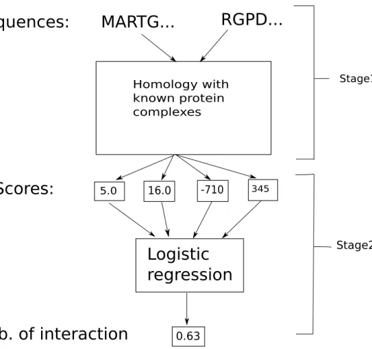
Homology with known protein complexes Stage1 Stage2

Figure 2-1: Struct2Net algorithm. The input to the algorithm are two protein sequences. The first stage consists of identifying the best complex template for the two proteins, and alignment of the proteins to the template using DBLRAP (Double RAPTOR) [177, 143]. In stage 2, a set of scores quantifying the quality of the alignment and predicted interface are extracted from the sequence-structure alignment of stage 1 and input into a classifier that predicts the probability of interaction.

(59)

the template database using RAPTOR [177], and the best template is chosen based on the alignment score. The alignments to the best template give us the predicted interface for the two sequences. Using this alignment and the interaction pattern be-tween the complex’s constituent subunits, we can also calculate the interfacial energy between our input proteins. The interfacial potential parameters are taken from Lu, Lu, and Skolnick’s paper[102].

In summary, for any given sequence pair (p and q), the threading-based

inter-face prediction method will generate two alignment scores (Ep, Eq), their associated

z-scores (zp,zq) , and an interfacial energy (Epq) evaluated using the statistical

poten-tial. z-scores measure the significance of the alignment score, with the background distribution of alignment scores computed by randomizing the residues at the aligned positions. This vector of scores is then used to represent the predicted interface (Figure 2-1).

From predicted interface to interaction probability

Struct2Net uses a binary logistic regression to classify whether a set of interface scores (from above) corresponds to an interaction or not. In binary logistic regression, the goal is to predict a binary output variable Y, given a set of r predictor variables X =X1, X2...Xr. For an instancei, supposeyi and xi =xi1, x2i, ...xri are the random

variables corresponding to Y and X respectively. Let θi = P(yi = 1|xi). In this

model, the dependence ofθi onxi is expressed by the logit function:

logit(θi) =log( θi

1−θi

) = α+βTxi =α+β1x1i+β2x2i+...+βrxri (2.1)

Structure-based algorithms for protein-protein interaction prediction

Structure-based algorithms for protein-protein

interaction prediction

by

Raghavendra Hosur

Submitted to the Department of Materials Science and Engineering

in partial fulfillment of the requirements for the degree of

Doctor of Philosophy

at the

MASSACHUSETTS INSTITUTE OF TECHNOLOGY

June 2012

© Massachusetts Institute of Technology 2012. All rights reserved.

Author . . . .

Department of Materials Science and Engineering

May 17, 2012

Certified by. . . .

Bonnie Berger

Professor of Applied Mathematics

Thesis Supervisor

Accepted by . . . .

Prof. Gerbrand Ceder

Chairman, Department Committee on Graduate Students

Structure-based algorithms for protein-protein interaction

prediction

by

Raghavendra Hosur

Abstract

Publications

Acknowledgments

Contents

List of Figures

List of Tables

Abbreviations

Glossary

Chapter 1

Introduction

1.1

Proteins

1.1.1

Protein structure determination

1.2

Protein-protein interactions

1.2.1

Types of PPIs

1.2.2

Structural features

1.2.3

Physico-chemical features

1.2.4

Evolutionary features

1.3

Experimental methods for PPI detection

1.3.1

Low throughput screens

1.3.2

High throughput screens

1.3.3

Limitations of experimental techniques

1.4

Computational methods for PPI prediction

1.4.1

Indirect methods

1.4.2

Direct methods

1.4.3

Data integration methods

GO

Random forest

classifier

True/False

1.5

Medical impact

1.6

Organization of the thesis

Chapter 2

Struct2Net: structure-based approach

to PPI prediction

2.1

Background

2.2