ISBN 978-82-471-2654-7 (printed ver.) ISBN 978-82-471-2655-4 (electronic ver.) ISSN 1503-8181 NTNU Norw egian Univ er sity of Scienc e and T echnol ogy Thesis f or the degr ee of phil osophiae doct or e and T echnol ogy gy and Pr oc es s Engineering
Doct
or
al theses at NTNU, 2011:64
Vladislav Efros
Structure of turbulent boundary
layer over a 2-D roughness
Thesis for the degree of philosophiae doctor
Trondheim, February 2011
Norwegian University of
Science and Technology
Faculty of Engineering Science and Technology
Department of Energy and Process Engineering
Abstract
The roughness is an important parameter in wall-bounded flows, as most surfaces
are rough. The main effect of the roughness is to increase the drag as the near wall
is affected by the roughness. In recent years a lot of efforts has been used to find
out what effect has the roughness on the outer layer. In other words is there any
differences in outer layer, boundary layer or channel flow, between rough and
smooth-surface?
Jimenez (2004) suggests that forδ/k> 40 there are no differences, in agreement
with Townsend’s hypothesis, the roughness merely acts to increase the surface stresses, without changing the structure in the flow.
This was challenged by Krogstadet. al(1999) who showed, for boundary layer
over 2−Droughness, there is a difference in the outer layer due to the roughness.
However for a channel flow Krogstadet.al(2004) has found no differences.
The main impediment is how to obtain a reliable estimate for the friction velocity,
uτ, which is the main scaling parameter of principal interest. In channel flow
theuτmay be obtained directly from the stream-wise pressure gradient. A
com-mon technique for boundary layer over smooth surface is the Clauser chart. This method is subjected to large uncertainties for rough surface, because the number
of unknowns is increased from one,Cf, for smooth surface to three, (Cf, , the
shift in origin andΔu/uτshift in velocity), for rough surface.
The need for an independent measurement of the wall shear stress has led to the present work.
A floating-balance has been designed to obtain the shear stress on the rough sur-face. The balance was tested in channel flow, adverse pressure gradient flow and zero pressure gradient boundary layer and the velocity field was investigated using a two-component LDA system. The results showed that the shear stress,
from balance, was underestimated by∼4%.
Turbulent boundary layer is a complicated nonlinear system; Clauser (1956) com-pared it with a black box. A better understanding of this system may be obtained by changing one of its inputs and to examine its output.
An experimental investigation on the response of a turbulent boundary layer to sudden change in roughness, from smooth to rough, using floating balance to measure the shear stress is also a part of the present work.
inves-Acknowledgments
I would like to express my thanks to my supervisor, Prof. Per-Åge Krogstad for all his support and guidance throughout these years. His practical ideas, during the period of building the balance, have been most valuable.
I would also like to thank John Krogstad and Arnt Egil Kolstad, laboratory staff,
for helping me to build all kind of devices necessary for the experimental part of this work.
Special thanks to Prof. Hyung Jin Sung and Assoc. Prof. Philipp Schaltter for providing the DNS data.
I also want to thank my colleagues for their help in the lab and for all the good time we had together.
Finally, I would like to thank my family for their love and support during this time. Most of all I would like to express my gratitude to Elen for her patience and love, no matter what.
Nomenclature
Roman
a, b,d distances
A1, A2 area
Axz projected area of the floating element in xz plane
B, C constants
c thickness of the gap
Cf skin friction coefficient,Cf =2 (uτ/Ue)2
D width of the floating element, D=50 mm
E recovered energy from POD modes
F shear force,F=τw·Axz
Fα flatness of componentα
FN force measured by balance
Fp pressure force
G Clauser’s shape parameter
g gap between the moving plate and surrounding wall
H shape parameter,H=θ/δ∗
h channel half height
K calibration constant
k hight of the roughness,k=1.7mm
L Length of the floating element, L=350 mm
Ruv correlation coefficient,Ruv =<−uv> /(σuσv)
Reθ Reynold number based on the momentum thickness,θ
Sα skewness of componentα
u stream wise velocity
Ue free stream velocity
uτ friction velocity,uτ= τw/ρ
u(Ln)(x,y) reconstructed velocity field from theNleading POD modes
u(Rn)(x,y) residual velocity field
X distance from the step to the measurement point
z0 roughness length, for a rough surfacez0=(ν/uτ)exp[−κ(A+ ΔU/uτ)]
Greek letters
β non-dimensional pressure gradient
ΔP pressure drop
ΔU+ vertical shift of the logarithmic curve
ΔX length
Δ Clauser’s thickness for turbulent layers,Δ =δ∗U
e/uτ
δ boundary layer thickness, defined asyfor whichu=0.99Ue
δi thickness of internal boundary layer
shift in origin
κ von Karman constant=0.41
λ roughness spacing
λci swirling strength
λi eigenvalue from POD
λs swirling strength with assigned sign based onωz
ν kinematic viscosity of the air
ω(Π,y/δ) wake function
ωz vorticity in (x,y) plane
φi POD modes
Π wake strength
ρ density of the air
σp standard deviation of componentp
τ total shear stress
θ momentum thickness
ks equivalent sand grain roughness
y spatial coordinate in spanwise direction
Superscripts
+ normalized withuτ
p coefficient in Elliot’s formula
Subscripts
l, m number of velocity components in a snapshot
p, q general index
Abbreviations
Contents
Abstract i
Acknowledgments iii
1 Introduction 1
1.1 Rough boundary layer . . . 1
1.1.1 The boundary layer concept . . . 1
1.1.2 Boundary layer over smooth surface . . . 2
1.1.3 Boundary layer over rough surface . . . 3
1.2 Skin Friction measurement . . . 5
1.2.1 Direct measurement . . . 5
1.2.2 Momentum balance . . . 6
1.2.3 Wall similarity technique . . . 7
1.3 The response of turbulent boundary layer to sudden perturbations 8 1.3.1 Sudden change in roughness . . . 9
1.4 Motivation . . . 10
1.5 References . . . 11
2 A Skin Friction Balance 13 2.1 Description of the balance . . . 13
2.2 Results . . . 19
2.3 Discussion and Conclusions . . . 24
2.4 References . . . 25
3 Turbulent boundary layer over a step change: smooth to rough. LDV measurements 27 3.1 Experimental set-up . . . 27
3.1.1 Wall-shear stress . . . 29
3.2 Results . . . 31
3.2.1 Mean flow . . . 31
3.2.2 Internal Boundary layer . . . 40
3.2.3 Reynolds stresses . . . 43
3.2.4 Transport equation for Reynolds stresses . . . 50
4.2.5 Proper orthogonal decomposition analysis . . . 102
4.2.6 Conlcusions . . . 115
4.3 References . . . 116
5 Summary and Conclusions 119
Chapter 1
Introduction
1.1 Rough boundary layer
1.1.1 The boundary layer concept
The concept of boundary layer was introduced by Prandtl and defined as - a thin
layer of fluid adjacent to the solid surface within which the viscous effects are
dominant. The velocity near the wall is smaller than at a large distance from it. The thickness of this layer is increasing along the flat plate in the downstream region (Schlichting (1968)). The velocity distribution over a flat plate is shown schematically in Figure (1.1). The boundary layer is a thin layer of retarded flow
Figure 1.1: Boundary layer over a flat plate (sketch)
of thicknessδwhich increases from the leading edge in the downstream direction.
The nominal thickness,δ, is the distance at which the velocity is 0.99Ue,Uebeing
the free stream velocity. The velocity approachesUeasymptotically andδis not
very easy to measure. Therefore the ill-definedδis substituted by more precisely
defined momentum thickness,θ, or displacement thickness,δ∗.
The displacement thickness,δ∗, is the displacement of the streamlines from the
wall compared to inviscid solution, in order to obtain the same mass rate of flow
as in the real case. From Figure (1.2) theδ∗can be defined:
∞ 0 udy= ∞ δ∗ Uedy⇒δ ∗= ∞ 0 1− u Ue dy (1.1)
Figure 1.2: Displacement thickness (sketch) From Figure (1.2) follows that the area A1 is equal with area A2.
The momentum thickness,θ, is defined as:
ρU2 eθ=ρ ∞ 0 (Ue−u)dy⇒θ= ∞ 0 u Ue 1− u Ue dy (1.2)
All of these thicknesses depend on the shape of velocity distribution. The ra-tio between the momentum thickness and displacement thickness is called the shape parameter, H.
H=δθ∗ (1.3)
1.1.2 Boundary layer over smooth surface
The main goal of the present work is to study the structure of the boundary layer over rough-surface but it is good to have an overview over boundary layer in zero pressure gradient over a smooth surface. The boundary layer over smooth surface must be divided into two regions; the inner region in which the viscosity is an important parameter and outer region where flow is independent of the viscosity. In the immediate vicinity of the wall we have
U uτ = y·uτ ν (1.4) where uτ= τwall ρ (1.5)
1.1. ROUGH BOUNDARY LAYER Further from the wall we have the logarithmic law of the wall
U uτ = 1 κln y·u τ ν +B (1.6)
This is universal in the inner layer which for flat plate boundary layer is considered asy/δ <0.2.
For the outer layer, log region, exist a universal relation between (Ue−u/uτ) and
y/δas Ue−u uτ = 1 κln y δ +C (1.7)
Outside the log region we have:
Ue−u uτ = f y δ (1.8)
The Karman constant,κ∼0.41 is considered to be universal. The constants B and
C are different from author to author, this might be connected with not enough
information about turbulent boundary layer.
1.1.3 Boundary layer over rough surface
Practically all surfaces are rough. The first rough-wall flow analysis was con-ducted by Nicuradze (1933), who investigated the flow in sand-roughened pipes.
He found that the flow depended on the relative scale of the roughnessk/d (k
is roughness scale and d pipe diameter) as well as the Reynolds number (Perry
et al). Flow dependent onk/dwas termed f ully roughwhile the flow dependent
on bothk/dand Reynolds number was termedtransition f low.
The main effect of the roughness is to increase the friction coefficient,Cf, and to
shift data with theΔU+compared to smooth data as shown in Figure (1.3) where
ΔU+is the vertical shift of the logarithmic curve caused by the roughness and has
the form (Clauser 1956)
ΔU+= 1 κln kuτ ν +const. (1.9)
Over either smooth or a rough wall the turbulent boundary layer consists of
an outer region (Raupach et al.) where the length scale is the boundary layer
thickness,δ, and a wall or inner region where the length scale isν/uτfor smooth
wall andν/uτtogether withkto characterize the rough wall. The velocity profiles
for rough and smooth-surface in outer coordinates are shown in Figure (1.4). The main conclusion from Figure (1.3) and Figure (1.4) is that
• in inner coordinates there is a region where the velocity profile is logarithmic
Figure 1.3: Velocity profile in inner coordinates
1.2. SKIN FRICTION MEASUREMENT
• in outer coordinates the equation (1.7) is valid for both smooth and rough
surface this indicate that the flow is similar in outer layer.
How is that possible a flow with different structure in inner layer could be similar
in outer layer?
U(y) is a function ofyno doubt but we should be careful in defining the origin of
yfor rough wall. The origin ofycan be taken anywhere between the crest of the
roughness and the valley of roughness. The distance,, defines the origin ofyfor
profiles that will give a logarithmic distribution near the wall (Perryet al).
1.2 Skin Friction measurement
Any object moving through a fluid experiences a drag that can be decomposed in pressure drag and skin friction drag. The problem of estimating turbulent skin friction is important in many applications, such as aerospace research or the structure of turbulent boundary layer. The shear stress is an important parameter for the normalization of the velocity profiles. Only with accurate measurement of the shear stress it is possible to establish reliable data for comparison with numerical simulations or models.
Several methods for measuring the shear stress in the wall have been developed. There is not a universal method to measure skin-friction because each problem
requires a specific geometry to be adapted and different techniques apply better
in different cases. Winter shows a review of the techniques used from 1940 to
1975 and range conditions required on each case. The modern developments are presented by Naughton & Sheplak. The principal skin-friction techniques are:
• Direct measurement
• Liquid tracers
• Momentum balance
• Wall similarity technique
• Microelectromechanical systems (MEMS) technique
• Thin-oil-film techniques
1.2.1 Direct measurement
Direct measurement is a method, which gives the shear stress directly without any assumptions about the flow. The skin friction balance is a direct measurement of the skin friction. This is very simple and well established technique but with many problems in practical application. A principle sketch of skin friction balance is
Figure 1.5: Floating element
for rough surface, consist of a frictional forceF,F=τw·Axz, whereτwis the wall
shear stress acting on the surface of the balanceAxzand the pressure forces acting
on the frontal area of the roughness,Fp. What we measure is the forceFNor the
displacement of the floating element. Usually the measured force is determined as
FN=K· τw·Axz+Fp
(1.10) where K is a calibration constant, which is determined by applying known loads and measuring the displacement or the force of the floating element.
The main problems (Winter 1977), which should be considered:
• A device to measure very small forces or displacements
• The effect of the gaps around the floating element
• Forces arising from the pressure gradients
• The effects of misalignment of the floating element
• Effects of temperature changes and vibrations from the tunnel
• Effects of leaks
1.2.2 Momentum balance
For the flows in constant area ducts, such as channels or pipes the wall shear stress can be obtained form the pressure gradient.
1.2. SKIN FRICTION MEASUREMENT
wherehis either the pipe radius or channel height,ΔPis the pressure drop over a
lengthΔX(Haritonidis 1989). This method is limited because it applies to a rather
special type of flow and because the flow should be fully developed. However it is ideal for calibration. (see Haritonidis 1989)
The application of the momentum balance to developing flow is less satisfactory. In principle it is simple you have to use the momentum integral equation and to
solve forτwall. The main drawback is that the equation contains some derivatives
(Brown & Joubert 1969) of slowly varying quantities, such as the momentum
thick-ness of the boundary layer. These derivatives are very difficult to be determined
accurately.
1.2.3 Wall similarity technique
In has been accepted that near the wall, for smooth wall andy+<5, the velocity
distribution is given byU+ = y+and hence the value of the skin friction can be
determined. This implies that we should measure very close to the wall in the viscous sub-layer. This sub-layer is very thin for high Reynolds number so the velocity cannot be determined correctly. Instead the logarithmic region is used. The log-law for smooth surface is presented bellow:
U uτ = 1 κln yu τ ν +B (1.12)
The main problem with equation 1.12 is the universality of constants,κand B. The
equation 1.12 is determined from the dimensional analysis while the constantsκ
and B are determined experimentally. Several authors have challenged the
con-stantsκand B, Österlund & Johansson determinedκ=0.38 and B=4.1.
The log law for rough surface, which is different from the meteorological
commu-nity, may be written
U uτ = 1 κln ⎛ ⎜⎜⎜⎜ ⎜⎜⎝ y+uτ ν ⎞ ⎟⎟⎟⎟ ⎟⎟⎠+B−ΔU+ (1.13)
Hereis the shift in origin of the effective wall location andΔU+is the shift in the
log law due to the roughness effect on the mean flow. The two addition unknowns,
andΔU+, for rough surface makes the fitting procedure more challenging. If
uτis determined in an independent way, this will decrease the uncertainty of the
remaining two variables in the fitting procedure. Other methods using the wall similarity technique are:
• Heat transfer
• Mass transfer
roughness elements. This was done by Perryet al. (1969) and by Antonia & Luxton (1971) for square transverse bars. For a more general rough surface it is necessary to use a balance to measure the force acting on a small area of surface. The direct measurement of skin friction on a rough surface was performed earlier
by Karlsson (1980) or Acharyaet al(1986).
1.3 The response of turbulent boundary layer to
sud-den perturbations
The turbulent boundary layer involve a complex combination of phenomena, the relatively simple case is the constant pressure boundary layer (Clauser 1956). We are interested to know what happens to the flow when the boundary layer is subjected to a sudden perturbation. The flow subjected to sudden perturbations is very often observed in nature. For example, when breezes encounter the coastline,
the sudden change in roughness can have an important effect on the flow (Smits &
Wood 1985). Another possible perturbations can be a sudden change in pressure gradient or the curvature of the surface, blowing or suction of the flow applied along a surface to control the flow. Apart form the practical reasons; the study of behavior of a perturbed boundary layer is a way for better understanding of the structure of turbulent boundary layer. The mechanism of the boundary layer is
very complicated and difficult to understand. Our goal is to try to understand it
by applying a sudden perturbation and to try to see what is the response to this imposed condition. Following Tani (1968) there are two methods of introducing the perturbations into boundary layer:
• The perturbation is applied as a sudden change in pressure or of a wall
roughness
• The perturbation is introduced of an obstacle in the flow or by the application
1.3. THE RESPONSE OF TURBULENT BOUNDARY LAYER TO SUDDEN PERTURBATIONS
1.3.1 Sudden change in roughness
Surface roughness can change from smooth to rough or rough to smooth. The work presented in this thesis is connected with the perturbation as a sudden change of a wall roughness, from smooth to rough.
The change in surface roughness is presented in Figure (1.6). When the turbulent
Figure 1.6: Sudden change in roughness
boundary layer flow run over a discontinuity in roughness is not anymore in
equilibrium. The region affected by the step change in roughness is called internal
boundary layer,δi. The boundary layer, upstream the step, is considered to be
fully developed and described by the equation (see Smits & Wood 1985):
U uτ = 1 κln y z0 (1.14)
wherez0is the roughness length. For a smooth wall we have:
z0smooth = ν uτ exp[−κB] (1.15)
For a rough surface,
z0rough= ν uτ exp −κ B+ΔU uτ (1.16)
The size of the step change can be measured byM∗=z01/z02, Smits & Wood (1985),
or byM= lnM∗, where 1 and 2 refers to the upstream and downstream values.
ForM<0 we have a step change from smooth to rough and forM>0 we have a
step change from rough to smooth.
According to Wood (1981) a general correlation for δi after a step change in
roughness for zero pressure gradient boundary layer is
δi z0 = f1 M∗,X z0 (1.17)
whereXis the distance from the step;z0can be eitherz01orz02. The equation
effect of the roughness, as mentioned above, is to increase the skin friction and to
shift data withΔU+. Although a lot of experiments have been done, one of the
first being Nikuradze, the boundary layer over rough surface is far from being elucidated.
The boundary layer over smooth or rough walls consists of outer and inner layer. According to Townsend’s hypothesis the turbulence outside the roughness
sublayer is unaffected by surface condition. This implies that the Reynolds stresses
(Flacket al.2005) normalized withuτ are universal outside the roughness
sub-layer. The roughness sub-layer extends∼(3−4)kfrom the wall. This is supported
by Flacket al.(2005), mesh and sand grain roughness, Volinoet al.(2007), Wu &
Christensen (2007), wall with replicated turbine blade roughness.
For 2−Droughness,k=1.7 mm andλ/k=8, Lee & Sung (2007) DNS, Volinoet al.
(2009) have found changes in the turbulence in the outer layer which is consistent
with Krogstad & Antonia (1999),λ/k=4,λis the roughness spacing.
Following the Jiménez (2004) for k << δ and k/δ > 40 the wall similarity is
expected. The similarity is expected when scaling withuτwhich is very difficult
to determine correctly. The use of Clauser plot, is subjected to large uncertainties
(Acharya et al 1986) because the number of variables to be determined from
fitting procedure are:,ΔU+andC
f compared with one,Cf, for smooth surface.
To decrease the uncertainty it is necessary to have an independent measurement
ofCf.
The development of a floating element for rough surface, which allows to measure
independently theCf, followed by the measurement of the structure of rough
turbulent boundary layer using laser Doppler anemometry, LDA, and particle image velocimetry, PIV, will be addressed in present thesis.
1.5. REFERENCES
1.5 References
I. Tani, Review of some experimental results on the response of a turbulent bound-ary layer to sudden perturbations,
Computation of turbulent boundary layers 1968 FOSR-IFR-Stanford Conference. Volume I, (1968), pp. 483-494
A. J. Smits & D. H. Wood, The response of turbulent boundary layers to sudden
perturbations,Annu. Rev. Fluid Mech17, (1985), pp. 321-358
D. H. Wood, Internal boundary layer growth following a step change in surface
roughness,Boundary Layer Metheorology22, (1982), pp. 241-244
J. R. Garratt, The internal boundary layer- a review,Boundary Layer Metheorology
50, (1990), pp. 171-203
H. Schlichting, Boundary-Layer Theory,Sixth Edition
A. E. Perry, W. H. Schofield, & P. N. Joubert, Rough wall turbulent boundary
layers,J. Fluid Mech 37, (1969), pp. 383-413
M. R. Raupach, R. A. Antonia & S Rajagopalan, Rough-wall turbulent boundary
layers,Applied Mechanics Reviews44, no 1, (1991), pp. 1-25
R. J. Volino, M. P. Schultz & K. A. Flack, Turbulence structure in a boundary layer
with two-dimensional roughness,J. Fluid Mech 635, (2009), pp. 75-101
J. W. Naughton, M. Sheplak, Modern developments in shear-stress measurement,
Progress in Aeropsace Sciencevol 38, (2002), pp. 515-570
R. A. Antonia and R. E. Luxton, The response of a turbulent boundary layer to a
step change in surface roughness. Part 1. Smooth to roughJ. Fluid Mech,48, part
4, (1971), pp. 721-761
S. Dhawan, Direct Measurements of Skin Friction, Report 1121
J. H. Haritonidis, The measurement of Wall Shear Stress,Advances in Fluid
Me-chanics Measurements,45, (1989), pp. 229-261
K. C. Brown & P. N. Joubert, The measurement of skin friction in turbulent
bound-ary layers with adverse pressure gradients,J. Fluid Mech,35, part 4, (1969), pp.
Chapter 2
A Skin Friction Balance
The main problem that slowed down the understanding of the roughness effect
on the flow has been the difficulty to measure the skin friction. This quantity
is very important because it represents the main scaling parameter. In addition,
for the rough surface an independent measurement ofuτis essential for accurate
determination of theΔu/uτand shift in origin,.
This led to the development of the skin-friction balance and a set of measurements
to investigate how accurateuτcan be measured.
2.1 Description of the balance
We spent around three years in our endeavor to build a balance to measure shear stress for our rough wall. At the beginning it was a classical balance with springs and non-contact sensor or laser displacement sensor to measure the displacement of the floating element. The main problems with sensors were too much drift and low sensitivity. The main challenge with the balance is the electronic part because the forces or displacements are very small.
The system was designed around a standard, offthe shell, laboratory balance.
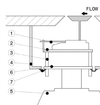
The balance is shown in the Figure (2.1). The device is a single-pivot type and consists of two main parts:
• The sensing element, which consists of a replica of the test surface (1) is
mounted on a thin plate. We have developed our balance for channel flow and two-dimensional boundary layer applications taking advantage of the spanwise homogeneity, so the sensing element is a rectangle with dimensions (DxL) 50x350mm in the streamwise and spanwise directions, respectively. The test plate is mounted on a vertical frame (2), which rests on a knife edge (6). Through the lower part of the frame is an adjustable horizontal bar (3) with two counter weights. The force is then transmitted to the sensing element through the adjustable vertical arm (4). By varying the ratio between arms (2) and (3) the "gain" of the system may be varied. Also
Figure 2.1: The skin friction balance.
balancing counter weights have been used to preload the sensing element of the balance to ensure that the balance always operates in its linear range.
• The balance (5) is a commercial force sensing unit from Ohaus with a
sensi-tivity of 0.001g. Normal loads are of the order of 12g and for these loads the
vertical motion of the sensing unit was less than 100μm as measured using
a micrometer dial gauge. The output from the balance was sampled on a computer through a RS232 connection.
In unloaded condition the sensing element was centered in the slot cut in the floor of the wind tunnel. The gap, g, between the movable plate and the surrounding
wall was nominally 0.6mm andg/D∼0.012.
Figure (2.2) shows the setup of the balance in wind tunnel. The whole balance could be positioned very accurately by means of three screws (3) controlling the vertical movement and two screws (1) that could be used to shift the balance in the horizontal plane. In addition the balance (5), Figure (2.1), has two more screw for fine adjustment in vertical direction
Figure (2.3) presents a sketch of the forces acting on the floating element, friction
force,F, lip force,LF, normal force,N, force due to the pressure on frontal area of
roughness,Fp, and the force measured by balance,FN. Following Allen (1976), the
sum of moments about the moment center, the following equation was obtained:
FN= a b Fp· 1+ k 2a +F+N·d a+ 1− c 2a ·LF (2.1)
2.1. DESCRIPTION OF THE BALANCE
Figure 2.2: The balance setup
The first two terms in equation 2.1 are the terms we want to measure, the first
term is zero for a smooth wall, for a rough wall the ratioFp/F >1, this indicate
that the main contribution to skin friction for rough wall is due to the pressure drag. The last two terms, representing the normal force and the lip force, should be zero for an ideal case. Thus this balance measure the total drag due to the pressure and the skin friction drag. The last two terms are main source of errors assuming that the calibration is perfect.
Figure 2.3: Forces acting on floating element
Because the balance is a single-pivot type, any normal force that does not pass through the pivot point will create a moment in addition to that from the skin
friction. The moment due to the normal force,N, are different from zero in two
cases:
• If the pressure above and bellow the floating element are not equal ( Allen
(1976))
• because the balance is a pivot type, any misalignment,d 0, will create a
momentum due to gravity force.
The moment due to normal force is not very big because the arm,d, usually is
very small compared with the length,a, arm for skin friction force.
Under ideal condition, when the protrusion is zero and the flow through the gap around the floating element (Allen (1976)) and the surrounding surface is null, the pressure around the floating element is constant creating no net force on the lip. As long as there is a flow through the gap a net force will be created.
In order to reduce the effects of any flow through the gaps, the balance was
mounted in a sealed box (4) fitted under the test surface; see Figure (2.2). To
minimize the effect of structural vibrations, a gap exists between the box (4) and
the plate (6); see Figure (2.2). This gap is sealed with a polyethylene film (7), Figure (2.2).
The lip force is mainly function of the protrusion of the element above and
be-low the surface. In our case we kept are negative protrusion of∼0.06 mm which
should be negligible in our case because we have a thick boundary layer (see Allen (1977)). We have a relatively big gap and this turns in our advantage because as
2.1. DESCRIPTION OF THE BALANCE Allen (1977) proved that the balance is less sensitive to protrusion errors at the larger gaps.
The pressure variation across the floating element will create a force in the di-rection of the skin friction force (see Hakkinen 2004), acting on the sides of the floating element (Figure (2.4)). Hakkinen (2004) has shown that the relative error caused by gap forces can be written as:
ε= dp/dx ·D·c τw·D = dp/dx·c τw (2.2)
whereτwis the shear force, dp/dx·c·D
is the net force,candDare the thickness
of the gap and the length of the floating element. The main conclusion from the
equation (2.2) is that the relative error is direct proportional with the gap depthc.
This explains why we have a sharp edge on the floating element and the surface
around the element (Figure 2.1). This is equivalent toc∼0.1mmsee Figure (2.3).
Figure 2.4: Gap forces.
The balance was calibrated in situ in the wind tunnel. The main problem in calibrating the balance was to generate a force, which is acting parallel with the sensing element. Using a calibrating device constructed in a similar way as the arms of the balance, except that it was inverted, solved this problem. The calibration device is presented in Figure (2.5). A frame (1), balanced by the weights (7), mounted on knife-edge supported by frame (2), which sits on the rough wall (4), is in contact with the floating element (5) through the arm (6). The vertical arm has a sharp edge at one end, which is in contact with one bar from the floating element. The container (3) is loaded with known masses necessary for calibrating. In this way the calibration device is transferring the vertical force due to weights to a force in the horizontal direction. The geometry of the calibration device doesn’t change during the calibration because the displacement of the floating element is negligible.
Figure 2.5: The calibration device.
The calibration curve obtained in this way is shown in Figure (2.6). The calibrated output is seen to be very linear with very little scatter. The ratio between the arms (2) and (3) in Figure (2.1) was adjusted to be close to 5:1 and this may be seen to be reflected in the five times higher output from the balance. The linear calibration
Figure 2.6: The calibration curve.
function fitted to the data was found to have a scatter typically better than 0.34% of full load.
Figure (2.7) shows theCf as function ofk+. For fully rough conditions,k+>60,
theCf should be constant. The differences between the averaged value, solid
line in Figure (2.7), and measured values, not for the first point, are∼ ±1%. The
differences for the first point is ∼ 2% this is connected with the fact that the
2.2. RESULTS
Figure 2.7:Cfversusk+.
2.2 Results
The main source of error is the pressure gradients (Hakkinen 2004); any small pressure gradient could be a significant source of error by creating a pressure
difference between upstream and downstream gaps. To check the performances,
the balance was exposed to three different pressure gradients.
The experiments were conducted in a closed return wind tunnel. Both the ceiling
and the floor was covered with square rods 1.7x1.7mm2. The pitch-to height ratio
λ/k=8 which correspond to "k-type roughness". In addition the upper wall of
the wind tunnel is adjustable.
Measurements of velocity field was performed using a Dantec two-components fiber-optic Laser Doppler Anemometry (LDA). In order to do near-wall measure-ments the probe was tilted at a small angle. The flow was seeded with small particles provided by Safex smoke generator. A total of 100 000 random velocity samples were obtained in coincidence mode for each location during the mea-surements. The probe was traversed to approximately 30 locations for case 1 and 40 locations for case 2 and 3. All the measurements were taken above the crest of the roughness elements.
To determine theuτthe balance was used. The data from balance was sampled as
long as velocity measurement. The moving average of the data from balance was
in the limit of±0.4%.
The variation of the non-dimensional pressure gradient (2.3) is shown in Table
2.2. β=h· 1 ρ·u2 τ · ΔPΔx (2.3)
τwch=h·
ΔP
Δx (2.4)
wherehis the half channel height anddP/dxis the pressure gradient. To measure
the pressure-drop, the test section is fitted with taps in the sidewall and along the centerline of the floor.
The axial mean-momentum equation for channel flow is:
−1ρdP dx +ν d2U dy2 − d dy <uv>=0 (2.5)
The integration of equation (2.5) from 0 toy
−ρydPdx −τw ρ + νdUdy−<uv> =0 (2.6) −1 u2 τ y ρ dP dx −1+ dU+ dy+−<uv+> =0 (2.7)
where superscript (+) means normalized with the shear stress,uτ, and the viscous
length scale,ν/uτ. The non-dimensional pressure gradient,β, can be included in
equation 2.7 and to obtain:
−<uv>+=1+β· y+ h+ −dU+ dy+ (2.8)
For a fully developed channel flowβshould be 1, but combining the pressure
gradient obtained from the taps and the shear stress obtained from balance,βwas
found to be slightly higher than one, 1.027. This indicate that the combined error in pressure and shear stress of less than 3%. The expected error from equation (2.2) is 0.2%.
For the adverse pressure-gradient we raised the roof, from 2h=280 mm to 2h=
600 mm at the exit, to form a diffuser. The angle of the diffuser was around 3.0
degrees. This allowed flow to develop under an adverse pressure gradient. There is no equilibrium condition in this case, so the only verification that can be used is that the normalized shear stress extrapolates to one at the wall.
2.2. RESULTS The last was the zero pressure gradient boundary layer. To obtain almost a zero pressure-gradient flow we changed the rough surface roof with a smooth surface roof and lifted the roof to avoid any interference between the boundary layer on the floor and roof of the tunnel. The roof was adjusted to obtain a zero pressure gradient. The mean velocity profiles for the three cases plotted in inner variables
are shown in Figure (2.8). All cases show a linear log region with a different
magnitude of wake strength. For the channel flow the shift was found to be,
ΔU+ ∼ 15 for k+ = 210, the shift for adverse pressure gradient, k+ = 107, and
boundary layer,k+=116, was found to be almost the same,ΔU+∼14.4.
The normal stresses in outer coordinates are shown in Figure (2.9) and Figure
Figure 2.8: Mean velocity,U+.−smooth,−−ΔU+=15 Symbols as in Tab.2.2.
(2.10). The stresses, at centerline, are independent of the pressure gradient in the
channel. The<uu>+and<vv>+, for adverse pressure gradient, are increased
throughout most of the outer layer compared with the channel and boundary layer. This is due to the increased turbulence production away from the wall in the case of the adverse pressure gradient. Figure (2.8) indicates that the slope,
dU+/dy, for adverse pressure is higher than for channel and boundary layer in the
outer layer. Combined with the increase in−< uv>+in the outer layer, Figure
(2.11), this increases the production term for< uu>+which indirectly increase
the<vv>+. The shear stress profiles are shown in Figure (2.11). For the channel
flow we have added the theoretical linear distribution defined by equation (2.8). The agreement is quite good giving confidence to the direct drag measurements. For the adverse pressure gradient the shear stress is seen to grow linearly near the wall as expected and data extrapolates back to 1 at the wall when scaled with shear stress obtained from the balance. For the zero pressure gradient profile, Figure (2.12), we have included the shear stress computed using the method described
Figure 2.9: Normal stress,uu+. Symbols as in Tab.2.2
Figure 2.10: Normal stress,vv+. Symbols as in Tab.2.2
2.2. RESULTS by Cebeci & Smith (1974),
τ τw =μ· ∂U ∂y −ρ·<uv>=1+ η 0 f2dη−f η 0 f dη 1 0 f 1−f dη (2.9)
where f =U/Ueandη=y/δ. A combined logarithmic law and a wake function
was used to represent the mean velocity profile,
U uτ = 1 κln yu τ ν +B+w Π,y δ (2.10)
wherew Π,y/δis the outer wake function and Granville’s function was used to
representw Π,y/δ, w Π,yδ= 1κ (1+6Π) y δ 2 −(1+4Π) y δ 3 (2.11) The agreement between the analytical and measured curve is seen to be good.
Figure 2.12: The shear-stress distribution,<uv>+. Thedenotes measured data
and the solid line denotes the analytical solution.
The correlation coefficient,Ruv = −<uv> /
√
<uu><vv>, looks almost iden-tical for the three flows. The flow for channel and adverse pressure gradient
collapse for y/δ > 0.2 see Figure (2.13). This is in agreement with findings of
Skåre & Krogstad (1994) that the correlation coefficient is very little affected by
Figure 2.13: The correlationRuv. Symbols as in Table 2.2
2.3 Discussion and Conclusions
The flow developing along the same rough surface, under fully developed chan-nel flow; an adverse pressure gradient and zero pressure gradient boundary layer conditions, was investigated using a two-component LDA system. The data ac-quired has been scaled with shear stress obtained from the direct measurement with a floating element.
For the channel flow the comparison was made with theoretical straight-line dis-tribution, the agreement was quite good. For the adverse pressure gradient the data is increasing linearly near the wall and the data set extrapolates back to one at the wall when scaled with balance measurements. The measurements done for the channel flow and zero pressure gradient boundary layer indicate that the nor-malized shear stress are slightly higher than 1. This suggests that the combined error in the shear stress, determined with balance, and pressure measurements of
∼4%. The relative error for channel flow,ε, calculated with equation (2.2) and
c=0.1mmis−0.2% while for adverse pressure gradient is+2.1%.
The presented balance, on rough walls, has proven to give reliable results under
different conditions. The balance has been used only for rough walls because the
shear stress is considered higher than for smooth wall. TheCfobtained in adverse
pressure gradient is almost twice the value expected for zero pressure gradient for smooth wall experiments. This imply that in order to get the same output for smooth wall we need to double the area of the floating element.
By using an "offthe shelf" micro force measurement unit, with proven accuracy
and stability, we have designed a balance with high accuracy and linearity. The results obtained from the balance are accurate and in good agreement with ana-lytical solution.
Despite this, further experiments with smooth surface are needed to establish the source of errors.
2.4. REFERENCES
2.4 References
P.-Å. Krogstad, R.A. Antonia and L.W.B. Browne, Comparison between
rough-and smooth-wall turbulent boundary layers,J. Fluid Mech. 245, (1992), pp. 599–
617
P.-Å. Krogstad, and R.A. Antonia, Surface roughness effects in turbulent
bound-ary layers,Exp. Fluids27, (1999), pp. 450-460
L. Keirsbulck, L. Labraga, A. Mazouz, and C. Tournier, Surface roughness effects
on turbulent boundary layer structure,J. Fluids Eng.124, (2002), pp. 127–135
K.A. Flack, M.P. Schulz, and T.A. Shapiro, Experimental support for Townsend’s
Reynolds number similarity,Phys. Fluids17, 035102, (2005)
S.-H. Lee, and H.J. Sung, Direct numerical simulation of the turbulent boundary
layer with rod-roughened wall,J. Fluids Eng.584, (2007), pp. 125–146
P.-Å. Krogstad, H. I. Andersson, O.M. Bakken, and A. Ashrafian, An experimental
and numerical study of channel flow with rough walls,J. Fluid Mech. 530, (2005),
pp. 327–352
A. Acharya and M. P. Escudier, Measurements of the Wall Shear Stress in Bound-ary Layer Flows, Turbulent Shear Flows 4,(1980), pp. 277-286
R. I. Karlsson, Studies of skin friction in turbulent boundary layers on smooth and rough walls, (1980)
K. A. Flack, M. P. Schulz and J. S. Connelly, Examination of a critical roughness
height for outlet layer similarity,Phys. Fluids19095104, (2007)
J. M. Allen, Experimental Study of Error Sources in Skin-Friction Balance
Mea-surements,Journal of Fluids Engineering99, (1977), pp. 197–204
R. J. Hakkinen, Reflections on Fifty Years of Skin Friction Measurement,AIAA
2004-2111pp. 1–13
P. E. Skåre, P-Å Krogstad, A turbulent equilibrium boundary layer near
separa-tion,J. Fluid Mech. 272, (1994), pp. 319–348da
H. Tennekes and J. L. Lumley, A First Course in Turbulence,The MIT Press, (1972)
T. Cebeci and A. M. O. Smith, Analysis of turbulent boundary layers,Academic
Chapter 3
Turbulent boundary layer over a step
change: smooth to rough. LDV
measurements
The interaction between the inner and outer layer in turbulent boundary layer is not well understood. A sudden change in roughness is used to study how a perturbation develops through the boundary layer and to see if it eventually changes the distributions of Reynolds stresses and high order moments in the outer layer.
3.1 Experimental set-up
The experiments were conducted in a closed return wind-tunnel. The upper wall is adjustable, which allows the adjustment of the pressure gradient. Because the
height of the exit section after contraction is only 280mmwe had to adjust the
upper wall as shown in Figure (3.1) with zero pressure gradient on the last half
(∼3m).
The experimental set-up being investigated consist of a rough wall, the same as
used by Krogstadet al.(2005), covered with a thin plate Figure (3.1) to make a
smooth wall followed by a rough wall of lengthX+200mm. The plate is placed
on top of rough elements so that the top of roughness is below the smooth surface
with 2mmthe thickness of the smooth plate.
For smooth wall case all the test section was covered with a smooth plate,X=0
means smooth-surface. Decreasing the length of the smooth plate will increase
the length, X, of the rough surface. This mean that the length of the smooth
surface is decreasing while the length of the rough surface is increasing.
The leading edge of the smooth plate, as shown in Figure (3.1), is bent to create a small ramp for the flow. The boundary layer is allowed to transition naturally without any wire trip.
forX=5.66mared =7.4,l =95.7.
The probe was traversed in vertical direction to approximately 35 positions using a Mitutoyo traverse. The data were collected in coincidence mode, 50 000 samples
forX=0 and 100 000 forX>0. The flow was seeded with∼1μmsmoke particles.
All the measurements were taken above the crest of the roughness element as in
the previous study of Krogstadet al.(2005).
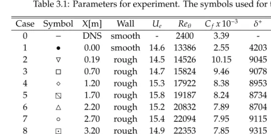
3.1. EXPERIMENTAL SET-UP Table 3.1: Parameters for experiment. The symbols used for the plots.
Case Symbol X[m] Wall Ue Reθ Cfx10−3 δ+ k+ k+s/k+
0 − DNS smooth - 2400 3.39 - - -1 • 0.00 smooth 14.6 13386 2.55 4203 - -2 0.19 rough 14.5 14526 10.15 9045 117.3 9.1 3 0.70 rough 14.7 15824 9.46 9078 114.4 10.1 4 1.20 rough 15.3 17922 8.38 8953 112.1 8.4 5 1.70 rough 15.8 19187 8.24 8734 115.2 10.0 6 2.20 rough 15.2 20832 7.89 8704 106.7 13.3 7 ◦ 2.70 rough 15.4 22094 7.95 9115 110.1 13.7 8 3.20 rough 14.9 22353 7.85 9315 106.2 10.3 9 3.82 rough 15.3 24802 7.06 9911 103.1 10.9 10 4.82 rough 15.3 28384 7.28 12057 104.8 10.8 11 5.66 rough 15.4 32624 6.78 13292 101.6 12.2
3.1.1 Wall-shear stress
The major problem when analyzing rough surface boundary layer experiments is to determine the friction velocity correctly. There are few techniques for rough surfaces based on the modified Clauser plot. The main problem is a large un-certainty because the number of quantities to be determined, for rough surface, is high compared with smooth surface and in addition the method is based on the existence of the logarithmic region. To avoid all this uncertainties we have
designed a floating element device (Efros & Krogstad (2009)) to measure theCffor
rough surfaces. The friction velocity on the smooth wall is determined by fitting
data to log-law. TheCf obtained from the floating element device is shown in
Figure (3.2). There is a sudden jump ofCffrom smooth to rough surface, followed
by a decrease towards a full rough-surface value. First the velocity field is slowed
down by new surface condition andCf is increasing. ThenCf is decreasing due
to flow adjustment the new surface. The trend of Cf denotes that the flow is
3.2. RESULTS
3.2 Results
3.2.1 Mean flow
The mean velocity profiles for smooth and rough surfaces are presented in Figure (3.3). The mean velocity profile, described by logarithmic-law, was calculated as,
U uτ = 1 κln ⎛ ⎜⎜⎜⎜ ⎜⎜⎝ y+uτ ν ⎞ ⎟⎟⎟⎟ ⎟⎟⎠+B−ΔU+ (3.1)
where is the shift in origin from the measurement coordinate system to the
effective wall location andΔU+ is the shift in the log law due to the roughness
effect on the mean flow. In our experiment the log-law constantsk=0.41,B=5.2,
= 0 and the origin of y is at the bottom of the groove, see Figure (3.1). The
variation ofΔU+andδ/kvs. k+are depicted in Figure (3.4) and Figure (3.5). The
shift in log law is almost constant for all cases.
Figure 3.3: Mean-velocity distribution for smooth- and rough-surfaces. Symbols:
−DNS smooth,•X=0,0.2,0.7,1.2,1.7,2.2,◦2.7,3.2,3.8,4.8,
5.66.
The velocity-defect profiles as a function ofy/δandy/Δare plotted in Figure (3.6).
whereΔ = δ∗·U
e/uτ. Note that the thickness of the boundary layerδcannot be
Figure 3.4: Shift in mean velocity,ΔU+vs.k+.
3.2. RESULTS
when the data is plotted as function ofy/Δ. This is because:
Δ =δ∗Ue uτ = ∞ 0 Ue−u uτ dy⇒ ∞ 0 Ue−u uτ d y Δ =1 (3.2) and Δ δ = δ∗ δ Ue uτ = 1+ Π κ (3.3)
For more detailes about how to obtain equation (3.3) see Castro (2007). Therefore
if the wakes are the same andReθsufficiently high you will always get a complete
collapse.
A combination between δ and δ∗ is the velocity scale, (U
eδ∗/δ), proposed by
Zaragola & Smits (1998) which is similar to one proposed by Rotta (1962).
Ueδ ∗ δ = ∞ 0 (Ue−u)d y δ ⇒ ∞ 0 Ue−u uτ d yuτ δ∗Ue =1 (3.4)
Velocity-defect profiles, using Zaragola & Smits scaling, are presented in Figure (3.7). The collapse of the velocity profiles using Zaragola & Smits scaling is quite
good and shows no effect of roughness except near the wall. Again, this method
guarantees collapse ifΠ(y/δ) is the same and can only distinguish differences in
the shape of the wake.
The scaling of velocity-defect profiles usingUe as scaling parameter is also
in-cluded in Figure (3.7). The profiles depicted in Figure (3.7) show no collapse
of data. This is in agreement with Akinladeet al.(2004), who showed that the
roughness is eliminated when the defect profile is scaled withUeδ∗/δand that the
effect of roughness is more evident when the defect profile is scaled withUe.
The Clauser’s shape parameter is defined as,
G=Δ1 ∞ 0 Ue−u uτ 2 dy (3.5)
and has a value of 6.8 for constant pressure turbulent boundary layers (Clauser
1956) andReθ >10·103(Bandyopadhyay 1992). ForX>2.7mthe value ofGfor
rough surfaces is about 6.5 which is slightly lower than the measured value for
smooth surface,X=0, which is 6.7. Using the value ofG=6.6 an indirect check
was carried out using the equation:
H= ⎡ ⎢⎢⎢⎢ ⎣1−G C f 2 0.5⎤ ⎥⎥⎥⎥ ⎦ −1 (3.6)
Figure 3.6: Velocity defect profiles , vs.y/δandy/Δ. Symbols:•X=0,0.2,0.7,
3.2. RESULTS
Figure 3.7: Velocity defect profiles. a) Zagarola & Smits scaling b) George &
Castillo. Symbols:•X=0,0.2,0.7,1.2,1.7,2.2,◦2.7,3.2,3.8,4.8,
Figure 3.8: Skin-friction results obtained from balance compared with the eqn(3.6)
ForX>2.2ma good agreement is obtained between equation (3.6) and
mea-sured value see Figure (3.8). The Figure (3.8) confirms the relation betweenHand
Cf(see equation (3.6)) but only for fully developed flows.
The displacement thicknessδ∗and the momentum thicknessθdepicted in
Fig-ure (3.9) have almost linear increase withX. The deviation of the displacement
thickness,δ∗, from the linear trend shown in Figure (3.9) is in agreement with the
velocity defect-law (see Figure (3.6)). This reveals that the retardation of the flow
due to the wall effects are constant forX>1.7mand flow develops differently.
Following Rotta (1962) the relation between the friction coefficient, Cf, and
displacement thickness,δ∗, can be written:
2 Cf = 1 κln ⎛ ⎜⎜⎜⎜ ⎜⎜⎝δk∗ 2 Cf ⎞ ⎟⎟⎟⎟ ⎟⎟⎠+const (3.7)
The skin friction plotted according to equation (3.7) are shown in Figure (3.10).
The data exhibit collapse, with experimental uncertainty, to a line with slope 1/κ.
3.2. RESULTS
Figure 3.9: Distribution ofδ∗(◦) andθ(•)
Figure 3.11: Momentum thicknessθ.
3.2. RESULTS
Using the relation betweenθandδ∗,
θ=δ∗ ⎛ ⎜⎜⎜⎜ ⎜⎝1−G Cf 2 ⎞ ⎟⎟⎟⎟ ⎟⎠ (3.8)
in equation (3.7) we can obtain:
2 Cf =− 1 κ ⎡ ⎢⎢⎢⎢ ⎢⎣lnk θ+ln ⎛ ⎜⎜⎜⎜ ⎜⎝1−G Cf 2 ⎞ ⎟⎟⎟⎟ ⎟⎠+1 2ln Cf 2 ⎤ ⎥⎥⎥⎥ ⎥⎦+const (3.9)
This equation gives a relation between skin friction,Cf, and momentum thickness,
θ, see Rotta (1962). This mean that being givenθas function ofXorX−X0,Cf
can be calculated as a function ofXor respectively as a function ofX−X0. Figure
(3.11) presents theθ = f(X−X0) data. TheCf = f(X−X0) usingG = 6.6 and
θ=0.0029(X−X0) obtained as best fit from Figure (3.11) is shown in Figure (3.12).
The trend between the calculated and experimental value is quite good except
for the first two points. It appears the the skin friction coefficient, Cf, can be
computed quite well based on the available distribution of momentum thickness.
The shape parameterH=δ∗/θis shown in Figure (3.13). It increases from a value
of 1.3 on smooth-surface to a maximum value of 1.76 forX= 2.2mand slowly
Figure 3.13: The shape parameterH.
3.2.2 Internal Boundary layer
ForX= 0, we have a fully developed turbulent boundary layer over a smooth
surface. Increasing the length,X, of rough surface changes the roughness of the
surface. The change in roughness is usually measured by the roughness step
M. The roughness step is defined asM = ln(z01/z02) wherez0is the equivalent
roughness length. The value forz0was determined using the equation (3.10):
z0= uν τexp κ ΔU uτ −B (3.10)
The value obtained forX=0 isz01=0.0034mmand forX=5.66misz02=0.585
mm. With the value forz01andz02calculated from above we foundM=−5.15.
The value found by Antonia & Luxton (1971a) wasM= −4.6 which points out
that the perturbations due to the rough surface is higher in our case.
After a change in surface roughness an internal boundary layer develops down-ward of the discontinuity. The internal layer will be in equilibrium with the rough-surface while the outer layer will have the characteristics determined by
the smooth-surface. The internal layer depends on the lengthXand the type of
the rough surface. With increasing the lengthXwe expect the internal layer to
increase until there is no outer layer determined by the smooth-surface.
The height of the internal boundary layer has been defined and determined in many ways - e.g. Antonia & Luxton (1971a) used half-power method of plotting
3.2. RESULTS the edge of internal boundary layer. Using this method Antonia & Luxton (1971a)
obtained a growth rate of internal layerδi ∼ x0.72. In our case the thickness of
internal layerδiwas determined, similar to Krogstad & Nickels (2006), by fitting
the internal and outer layer of stream wise stresses<uu >with a straight line.
The intersection of these two lines was considered the merging point of the two layers.
A fit to all points is given byδi∼x0.73, which is in good agreement with Antonia
& Luxton and close to the result of Krogstad & Nickels (2006)δi∼x0.7. The
vari-ation of boundary layer thickness and of internal boundary layer with length,X,
of rough surface is presented in Figure (3.14). The Figure (3.14) shows that the
internal boundary layer has grown to the edge of the boundary layer atX∼2.7m.
Figure (3.15) presents the data corresponding to Elliot’s (1958) formula for growth
Figure 3.14: The variation of boundary layer thicknessδ(•) and internal boundary
layer thiknessδi(◦) withX
of the internal boundary layer:
δi z02 =a X z02 p (3.11)
The coefficientawas calculated according to the relation (see Pendergrass & Arya
1984).
a=0.75−0.03M (3.12)
For the present experiment the magnitude ofacalculated with equation (3.12)
Figure 3.15: Comparison of the experimental developmentδi(•) with he theory
3.2. RESULTS
3.2.3 Reynolds stresses
The Reynolds stresses normalized with inner and outer variables are shown in Figure (3.16) to Figure (3.18) together with the results of smooth wall DNS by
Schlatteret al.(2009) atReθ =2400. Figure (3.16) shows the<uu+>component.
The maximum value of<uu+>, for smooth surface, is located aty+≈17 which
is in a good agreement with the DNS data. For X = 5.66mwe can notice that
< uu+ >is increasing from y+ ≈ 150 (1.35k) until it reaches a peak at y+ ≈ 700
(5.5k). The same can be noticed for X = 3.8mand X = 4.8m. From the DNS
(see Sunget al.2007) we know that there is a peak near the wall followed by a
valley and a second peak further from the wall. Our measurements show the
second peak and suggest the possibility to have a minimum at y+ ≈ 150. The
second peak, for high Renolds number, was noticed also by Marusicet al.2009
and Metzgeret al.2007. Marusicet al.2009 associated the second peak with very
large-scale structure, while Metzgeret al.2007 associated it with roughness effect.
For low Reynolds number, the second peak for rough-surface was noticed in the
DNS (Sunget al.2007), but only over the roughness element. It is evident that the
second peak for smooth surface is an effect of the high Reynolds number while
for the rough-surface we have in addition the effect of the roughness.
Increasing the length of rough-surfaceXaffects the<uu+>in two ways.
First, the peak,max(<uu+>), increases in magnitude with increasing the length
X, from 3.5 atX =0.2mto 5.2 atX= 5.66m, and moves fromy+≈255 (2.2k) at
X=0.2 toy+≈723 (7k) atX=5.66m.
Second, the< uu+ >extends progressively further into outer layer of initially
boundary layer over smooth surface asXis increasing. The second observation is
valid also for<vv+>and<uv+>component. The streamwise Reynolds stresses,
<uu+>, in outer variables, show good agreement between the rough-,X>1.7m,
and smooth-surfaces in the region 0.15 < y/δ < 0.9. This is in agreement with
Flacket al.(2007) and with the data discussed by Raupachet al.(1991).
The fluctuating component v, normal to the wall, provides information about
the turbulence transport and production of shear stress. Figure (3.17) shows the
<vv+>component in inner and outer variables. Reynolds number similarity is
noticed fory+< 150, for smooth surface, with good agreement between
experi-ment and DNS.
The change in surface will create a peak in< vv+ > at around y+ = 200 (1.8k),
X=0.2m, followed by a drop. The peak near the wall forX >0 is a
character-istic of the roughness and is in agreement with DNS of Sunget al.(2007). The
position of near wall peak for< vv+ >is close to the position of minimum for
<uu+ >which indicate that the reduction in<uu+>has been compensated by
the increase in<vv+>. Increasing further the lengthXof the rough surface will
create a plateau which forX >2.7mwill result in a second top,y/δ ≈0.2. For
is a significant part in the production term for the kinetic energy (Fernholz &
Finley (1996)). The<uv+ >component in inner and outer variables is shown in
Figure (3.18). Similar to<vv+ >, for smooth surface, the data collapse well for
y+<150. The maxim value for−<uv>+obtained from measurements forX=0
is∼ 0.96 which is similar to the value∼0.95 obtained by DNS (see Schlatter &
Örlü 2010). This indicate that the measurements are not affected by any probe
effects (Fernholz & Finley (1996)). The change in surface,X= 0.2m, will create
a peak in<uv+ >close to the position of the first peak in<vv+ >. Increasing
further the length,X, of the rough surface the< uv+ >will display a plateau
similar to the smooth surface. ForX=5.66mthe plateau extends fromy+≈200
(1.8k) toy+≈2000 (19k).
The effect of roughness on outer flow is small when the velocity is scaled with
uτ. To make the effect of roughness more evident the results are normalized with
Ue. The longitudinal and vertical stresses normalized withU2e are shown in
Fig-ure (3.19). With increase in the length, X, of the rough surface the profiles are
shifted upward making a clear distinction between smooth and rough surface. It is observed that the increase in Reynolds stresses is delimited by the thickness
of internal layerδi. ForX>2.2mthe flow has fully recovered from the effect of
the roughness. Near the wall the peak of< uu > /U2
e is almost constant while
the peak for< uv> /U2
e and<vv > /U2e overshoots the equilibrium value and
decreases with increasingXtowards the value of full rough surface. The same
was noticed by Pendergrass & Arya (1984). The− < uv >profiles normalized
withU2
e are presented in Figure (3.20). The distribution of−< uv>shows the
3.2. RESULTS
Figure 3.16: Streamwise normal stress, < uu+ > vs. y/δ and y+. Symbols:
M DNS smooth surface, −− DNS rough surface, • X=0, 0.2, 0.7, 1.2,
Figure 3.17: Wall-normal stress, < vv+ > vs. y/δ and y+. Symbols:
MDNS smooth surface, −− DNS rough surface, •X=0, 0.2, 0.7, 1.2,
3.2. RESULTS
Figure 3.18: Shear stress,−<uv+>vs. y/δandy+. Symbols:MDNS smooth,−−
DNS rough surface,•X=0,0.2,0.7,1.2,1.7,2.2,◦2.7,3.2,3.8,4.8,
Figure 3.19: Reynolds stresses normalized withU2
e . Symbols:•X=0,0.2,0.7,
3.2. RESULTS
Figure 3.20: Shear stress profiles normalized withU2
e . Symbols: •X=0,0.2,