ADAPTIVE NONLINEAR SYSTEM IDENTIFICATION
AND CHANNEL EQUALIZATION USING
FUNCTIONAL LINK ARTIFICIAL NEURAL NETWORK
A THESIS SUBMITTED IN PARTIAL FULFILLMENT OF THE REQUIREMENTS FOR THE DEGREE OF
Master of Technology
in
Telematics and Signal Processing
By
AJIT KUMAR SAHOO
Department of Electronics and Communication Engineering
National Institute Of Technology
Rourkela
ADAPTIVE NONLINEAR SYSTEM IDENTIFICATION
AND CHANNEL EQUALIZATION USING
FUNCTIONAL LINK ARTIFICIAL NEURAL NETWORK
A THESIS SUBMITTED IN PARTIAL FULFILLMENT OF THE REQUIREMENTS FOR THE DEGREE OF
Master of Technology
in
Telematics and Signal Processing
By
AJIT KUMAR SAHOO
Under the Guidance of
Prof. G. Panda
Department of Electronics and Communication Engineering
National Institute Of Technology
Rourkela
National Institute Of Technology
Rourkela
CERTIFICATE
This is to certify that the thesis entitled, “Adaptive Nonlinear System Identification and Channel Equalization Using Functional Link Artificial Neural Network” submitted by Sri Ajit kumar Sahoo in partial fulfillment of the requirements for the award of Master of Technology Degree in Electronics & communication Engineering with specialization in
“Telematics and Signal Processing” at the National Institute of Technology, Rourkela (Deemed University) is an authentic work carried out by him under my supervision and guidance.
To the best of my knowledge, the matter embodied in the thesis has not been submitted to any other University / Institute for the award of any Degree or Diploma.
Prof. G. Panda
Dept. of Electronics & Communication Engg. Date: National Institute of Technology
ACKNOWLEDGEMENTS
This project is by far the most significant accomplishment in my life and it would be impossible without people who supported me and believed in me.
I would like to extend my gratitude and my sincere thanks to my honorable, esteemed supervisor Prof. G. Panda, Head, Department of Electronics and Communication Engineering. He is not only a great lecturer with deep vision but also most importantly a kind person. I sincerely thank for his exemplary guidance and encouragement. His trust and support inspired me in the most important moments of making right decisions and I am glad to work with him.
I want to thank all my teachers Prof. G.S. Rath, Prof. K. K. Mahapatra, Prof. S.K. Patra and Prof. S.K. Meher for providing a solid background for my studies and research thereafter. They have been great sources of inspiration to me and I thank them from the bottom of my heart.
I would like to thank all my friends and especially my classmates for all the thoughtful and mind stimulating discussions we had, which prompted us to think beyond the obvious. I’ve enjoyed their companionship so much during my stay at NIT, Rourkela.
I would like to thank all those who made my stay in Rourkela an unforgettable and rewarding experience.
Last but not least I would like to thank my parents, who taught me the value of hard work by their own example. They rendered me enormous support during the whole tenure of my stay in NIT Rourkela.
Ajit Kumar Sahoo
CONTENTS
Page No. Abstract. i
List of Figures. iii
List of Tables. v Abbreviations Used. vi Chapter 1. Introduction. 1.1. Introduction. 1 1.2. Motivation. 1 1.3. Thesis Layout. 3
Chapter 2. Adaptive Modeling and System Identification.
2.1. Introduction. 4
2.2. Adaptive Filter. 5
2.3. Filter Structures. 7
2.4. Application of Adaptive Filters. 8
2.4.1. Direct Modeling. 8
2.4.2. Inverse Modeling. 10
2.5. Gradient Based Adaptive Algorithm. 10
2.5.1. General Form of Adaptive FIR Algorithm. 11 2.5.2. The Mean-Squared Error Cost Function. 11
2.5.3. The Wiener Solution. 12
2.5.4. The Method of Steepest Descent. 13
2.6. Least Mean Square (LMS) Algorithm. 14
2.7. System Identification. 16
2.8. Simulation Results. 17
Chapter 3. System Identification Using Artificial Neural Network (ANN).
3.1. Introduction. 22
3.2. Single Neuron Structure. 23
3.2.1. Activation Functions and Bias. 24
3.2.2. Learning Process. 24
3.3. Multilayer Perceptron. 26
3.3.1. Back Propagation Algorithm. 27
3.4. Functional Link ANN (FLANN). 29
3.4.1. Learning Algorithm. 30
3.5. Cascaded FLANN (CFLANN). 32
3.5.1. Learning Algorithm. 32
3.6. Simulation Results. 36
3.7. Summary 42
Chapter 4. Pruning Using Genetic Algorithm (GA).
4.1. Introduction. 43 4.2. Genetic Algorithm. 44 4.2.1. GA Operations. 45 4.2.2. Population Variable. 46 4.2.3. Chromosome Selection. 46 4.2.4. Gene Crossover. 48 4.2.5. Chromosome Mutation. 49 4.3. Parameters of GA. 50
4.4. Pruning Using GA. 51
4.5. Simulation Results. 55
4.6. Summary. 59
Chapter 5. Channel Equalization.
5.1. Introduction. 60
5.2 .Base Band Communication System. 61
5.3. Channel Interference. 61
5.4. Minimum and Nonminimum Phase Channels. 63
5.5. Inter Symbol Interference. 64
5.5.1. Symbol Overlap. 64 5.6. Channel Equalization. 65 5.6.1. Transversal Filter. 67 5.7. Simulation Results. 68 5.8. Summary. 70 Chapter 6. Conclusions. 6.1. Conclusions. 71
6.2. Scope for Future Work. 71
Abstract
In system theory, characterization and identification are fundamental problems. When the plant behavior is completely unknown, it may be characterized using certain model and then, its identification may be carried out with some artificial neural networks(ANN) like multilayer perceptron(MLP) or functional link artificial neural network(FLANN) using some learning rules such as back propagation (BP) algorithm. They offer flexibility, adaptability and versatility, so that a variety of approaches may be used to meet a specific goal, depending upon the circumstances and the requirements of the design specifications. The primary aim of the present thesis is to provide a framework for the systematic design of adaptation laws for nonlinear system identification and channel equalization. While constructing an artificial neural network the designer is often faced with the problem of choosing a network of the right sizefor the task. The advantages of using a smaller neural network are cheaper cost of computation and better generalization ability. However, a network which is too small may never solve the problem, while a larger network may even have the advantage of a faster learning rate. Thus it makes sense to start with a large network and then reduce its size. For this reason a Genetic Algorithm (GA) based pruning strategy is reported. GA is based upon the process of natural selection and does not require error gradient statistics. As a consequence, a GA is able to find a global error minimum.
Transmission bandwidth is one of the most precious resources in digital communication systems. Communication channels are usually modeled as band-limited linear finite impulse response (FIR) filters with low pass frequency response. When the amplitude and the envelope delay response are not constant within the bandwidth of the filter, the channel distorts the transmitted signal causing intersymbol interference (ISI). The addition of noise during propagation also degrades the quality of the received signal. All the signal processing methods used at the receiver's end to compensate the introduced channel distortion and recover the transmitted symbols are referred aschannel equalization techniques.
When the nonlinearity associated with the system or the channel is more the number of
branches in FLANN increases even some cases give poor performance. To decrease the number of branches and increase the performance a two stage FLANN called cascaded FLANN (CFLANN) is proposed.
This thesis presents a comprehensive study covering artificial neural network (ANN) implementation for nonlinear system identification and channel equalization. Three ANN structures, MLP, FLANN, CFLANN and their conventional gradient-descent training methods are extensively studied.
Simulation results demonstrate that FLANN and CFLANN methods are directly applicable for a large class of nonlinear control systems and communication problems.
LIST OF FIGURES
Figure No Figure Title Page No.
Fig.2.1 Type of adaptations 5
Fig.2.2 General Adaptive Filtering 6
Fig.2.3 Structure of an FIR Filter 8
Fig.2.4 Direct Modeling 9
Fig.2.5 Inverse Modeling 10
Fig.2.6 Block diagram of system identification 17
Fig.2.7 Response and MSE plot for linear system using LMS algorithm 18
Fig.2.8-2.11 Response and MSE plot for nonlinear systems using LMS algorithm 19
Fig.3.1 A single neuron structure 23
Fig. 3.2 Structure of multilayer perceptron 26
Fig. 3.3 Neural network using BP algorithm 27
Fig.3.4 Structure of the FLANN model 30
Fig. 3.5 Structure of CFLANN Model. 33
Fig.3.6-3.10 Response comparison between MLP and FLANN 37
Fig.3.11-3.12 Performance comparison between LMS, FLANN and CFLANN 41
Fig.4.1. GA Iteration Cycle 45
Fig.4.2. Biased roulette-wheel for the selection of the mating pool 47
Fig.4.3. Gene crossover 49
Fig.4.4 Mutation operation in GA 50
Fig.4.6 Bit allocation scheme for pruning and weight updating 54
Fig.4.7. Output plot for static and dynamic systems 58 Fig.5.1. A baseband Communication System 61 Fig.5.2. Impulse Response of a transmitted signal in a channel 62 Fig.5.3. Interaction between two neighboring symbols 65 Fig.5.4. Block diagram of Channel Equalization 66 Fig.5.5. Linear Transversal Filter 67 Fig.5.6. BER plot comparison between LMS, FLANN, CFLANN 69
LIST OF TABLES
Table No. TableTitle Page No.
3.1 Common activation functions. 24
4.1 Comparison of computational complexity between FLANN
and pruned FLANN structure for static systems. 56 4.2 Comparison of computational complexity between FLANN
ABBREVIATIONS USED
ANN Artificial Neural Network
BGA Binary Coded Genetic Algorithm (BGA)
BP Back Propagation
CFLANN Cascaded Functional Link Artificial Neural Network
DCR Digital Cellular Radio
DSP Digital Signal Processing
FIR Finite Impulse Response
FLANN Functional Link Artificial Neural Network
FPGA Field Programmable Gate Array
GA Genetic Algorithm
IIR Infinite Impulse Response
ISDN Integrated Service Digital Network ISI Inter Symbol Interference
LAN Local Area Network
LMS Least Mean Square
MLANN Multilayer Artificial Neural Network
MLP Multilayer Perceptron
MLSE Maximum Likelihood Sequence Estimator
MSE Mean Square Error
Chapter
1
1. INTRODUCTION
1.1. INTRODUCTION.
System identification is one of the most important areas in engineering because of its applicability to a wide range of problems.Mathmatical system theory, which has in the past few decades evolved into a powerful scientific discipline of wide applicability, deals with analysis and synthesis of systems. The best developed theory for systems defined by linear operators using well established techniques based on linear algebra, complex variable theory and theory of ordinary linear differential equations. Design techniques for dynamical systems are closely related to their stability properties. Necessary and sufficient conditions for stability of linear time-invariant systems have been generated over past century, well-known design methods have been established for such systems. In contrast to this, the stability of nonlinear systems can be established for the most part only on a system-by-system basis. In the past few decades major advances have been made in adaptive identification and control for identifying and controlling linear time-invariant plants with unknown parameters. The choice of the identifier and the controller structures based on well established results in linear systems theory. Stable adaptive laws for the adjustment of parameters in these which assures the global stability of the relevant overall systems are also based on properties of linear systems as well as stability results that are well known for such systems [1.1].
In recent years, with the growth of internet technologies, high speed and efficient data transmission over communication channels has gained significant importance. The rapidly increasing computer communication has necessitated higher speed data transmission over wide spread network of voice bandwidth channels. In digital communications the symbols are sent through linearly dispersive mediums such as telephone, cable and wireless. In band width efficient data transmission systems, the effect of each symbol transmitted over such time-dispersive channel extends to the neighboring symbol intervals. This distortion caused by the resulting overlap of received data is called intersymbol interference (ISI) [1.2].
1.2. MOTIVATION
Adaptive filtering has proven to be useful in many contexts such as linear prediction,
channel equalization, noise cancellation, and system identification. The adaptive filter attempts to iteratively determine an optimal model for the unknown system, or “plant”, based on some function of the error between the output of the adaptive filter and the output of the
plant. The optimal model or solution is attained when this function of the error is minimized. The adequacy of the resulting model depends on the structure of the adaptive filter, the algorithm used to update the adaptive filter parameters, and the characteristics of the input signal.
When the parameters of a physical system are not available or time dependent it is difficult to obtain the mathematical model of the system. In such situations, the system parameters should be obtained using a system identification procedure. The purpose of system identification is to construct a mathematical model of a physical system from input-output. Studies on linear system identification have been carried out for more than three decades [1.3]. However, identification of nonlinear systems is a promising research area. Nonlinear characteristics such as saturation, dead-zone, etc. are inherent in many real systems. In order to analyze and control such systems, identification of nonlinear system is necessary. Hence, adaptive nonlinear system identification has become more challenging and received much attention in recent years [1.4].
High speed data transmission over communication channels is subject to intersymbol interference (ISI) and noise. The intersymbol interference is usually the result of the restricted bandwidth allocated to the channel and/or the presence of multipath distortion in the medium through which the information is transmitted. Equalization is the process which reconstructs the transmitted data jointly combating the ISI and the noise in the communication link. The simplest architecture in the class of equalizers making decisions in a symbol–by–symbol basis is the linear transversal filter. The field of digital data communications has experienced an explosive growth in recent years and its demand reaches at the peak as additional services are being added to existing infrastructure. The telephone networks were originally designed for voice communication but, in recent times, the advances in digital communications using Integrated Service Digital Network (ISDN), data communications with computers, fax, video conferencing etc. have pushed the use of these facilities far beyond the scope of their original intended use. Similarly, introduction of digital cellular radio (DCR) and wireless local area networks (LAN’s) have stretched the limited available radio spectrum capacity to the limits it can offer. These advances in digital communications have been made possible by the effective use of the existing communication channels with aid of signal processing techniques. Nevertheless these advances on the existing infrastructure have introduced a host of new unanticipated problems. The conventional LMS algorithm [1.5] fails in case of nonlinear channels. Hence non-linear channel estimation is a key problem in communication
system. Several approaches based on Artificial Neural Network (ANN) have been discussed recently for estimation of nonlinear channels.
1.3. THESIS LAYOUT
In Chapter 2, adaptive modeling and system identification problem is defined for linear and nonlinear plants. The conventional LMS algorithm and other gradient based algorithm for FIR system are derived. Nonlinearity problems are discussed briefly and various methods are proposed for its solution.
In Chapter 3, the theory, structure and algorithms of various artificial neural networks are discussed. We focus on Multilayer Perceptron (MLP), Functional Link ANN (FLANN) and Cascaded Functional Link ANN (CFLANN). We discuss the learning rule in each of the methods. Simulation results are carried out for comparisons of ANN technique with conventional LMS method under different nonlinear condition and noise.
Chapter 4 gives an introduction to evolutionary computing technique and discusses in details about genetic algorithm and its operators. It also discusses various selection schemes for population and crossover. In this chapter Genetic Algorithm is used for simultaneous pruning and weight updation for efficient nonlinear system identification.
In Chapter 5, the adaptive channel equalization is defined for and nonlinear channels. Different kinds of communication channel and inter symbol interference is discussed. The performance of conventional LMS algorithm based equalizer and other ANN structures such as FLANN and CFLANN equalizer are compared.
Chapter 6 summarizes the work done in this thesis work and points to possible directions for future work.
Chapter
2
ADAPTIVE MODELING AND SYSTEM
IDENTIFICATION
2
. ADAPTIVE MODELING AND SYSTEM IDENTIFICATION
2.1. INTRODUCTION
Modeling and system identification is a very broad subject, of great importance in the fields of control system, communications, and signal processing. Modeling is also important outside the traditional engineering discipline such as social systems, economic systems, or biological systems. An adaptive filter can be used in modeling that is, imitating the behavior of physical systems which may be regarded as unknown “black boxes” having one or more inputs and one or more outputs.
The essential and principal property of an adaptive system is its time-varying, self-adjusting performance. System identification [2.1, 2.2] is the experimental approach to process modeling. System identification includes the following steps
• Experiment design Its purpose is to obtain good experimental data and it includes
the choice of the measured variables and of the character of the input signals.
• Selection of model structure A suitable model structure is chosen using prior
knowledge and trial and error.
• Choice of the criterion to fit: A suitable cost function is chosen, which reflects how
well the model fits the experimental data.
• Parameter estimation An optimization problem is solved to obtain the numerical
values of the model parameters.
• Model validation: The model is tested in order to reveal any inadequacies.
The adaptive systems have following characteristics
1) They can automatically adapt (self-optimize) in the face of changing (non-stationary) environments and changing system requirements.
2) They can be trained to perform specific filtering and decision making tasks. 3) They can extrapolate a model of behavior to deal with new situations after
trained on a finite and often small number of training signals and patterns. 4) They can repair themselves to a limited extent.
5) They can be described as nonlinear systems with time varying parameters. The adaptation is of two types
(i) open-loop adaptation
of input or environment characteristics, applying this information to a formula or to a computational algorithm, and using the results to set the adjustments of the adaptive system. The adaptation of process parameters don’t depend upon the output signal.
Processor Input signal
Output
signalOther data Adaptive algorithm (a) Processor Input signal
Output
signalOther data Adaptive algorithm Performance calculation (b)
Fig.2.1. Type of adaptations (a) Open-loop adaptation and (b) Closed-loop adaptation (ii) closed-loop adaptation
Close-loop adaptation, as shown in Fig. 2.1.(b),on the other hand involves the automatic experimentation with these adjustments and knowledge of their outcome in order to optimize a measured system performance. The latter process may be called adaptation by “performance feedback”. The adaptation of process parameters depends upon the input as well as output signal.
2.2. ADAPTIVE FILTER
An adaptive filter [2.3, 2.4] is a computational device that attempts to model the relationship between two signals in real time in an iterative manner. Adaptive filters are often realized either as a set of program instructions running on an arithmetical processing device such as a microprocessor or digital signal processing (DSP) chip, or as a set of logic operations implemented in a field-programmable gate array (FPGA). However, ignoring any errors introduced by numerical precision effects in these implementations, the fundamental operation of an adaptive filter can be characterized independently of the specific physical realization that it takes. For this reason, we
shall focus on the mathematical forms of adaptive filters as opposed to their specific realizations in software or hardware. An adaptive filter is defined by four aspects:
1. The signals being processed by the filter.
2.The structure that defines how the output signal of the filter is computed from its input signal
3.The parameters within this structure that can be iteratively changed to alter the filter's input-output relationship
4.The adaptive algorithm that describes how the parameters are adjusted from one time instant to the next.
By choosing a particular adaptive filter structure, one specifies the number and type of parameters that can be adjusted. The adaptive algorithm used to update the parameter values of the system can take on an infinite number of forms and is often derived as a form of optimization procedure that minimizes an error.
Adaptive Filter d(n) x(n)
Σ
y (n) e(n) +Fig.2.2. General Adaptive Filtering
Fig.2.2. shows a block diagram in which a sample from a digital input signal x(n) is
fed into a device, called an adaptive filter, that computes a corresponding output signal sample y(n) at time n. For the moment, the structure of the adaptive filter is not important, except for the fact that it contains adjustable parameters whose values affect how y(n) is computed. The output signal is compared to a second signal d(n), called the desired response signal, by subtracting the two samples at time n. This difference signal, given by
( ) ( ) ( )
e n =d n −y n (2.1) is known as the error signal. The error signal is fed into a procedure which alters or
adapts the parameters of the filter from time n to time (n + 1) in a well-defined manner. As the time index n is incremented, it is hoped that the output of the adaptive filter becomes a better and better match to the desired response signal through this adaptation process, such that the magnitude of e n( ) decreases over time. In the adaptive filtering task, adaptation refers to the method by which the parameters of the system are changed from time index n to time index (n +1). The number and types of parameters within this system depend on the computational structure chosen for the system. We now discuss different filter structures that have been proven useful for adaptive filtering tasks.
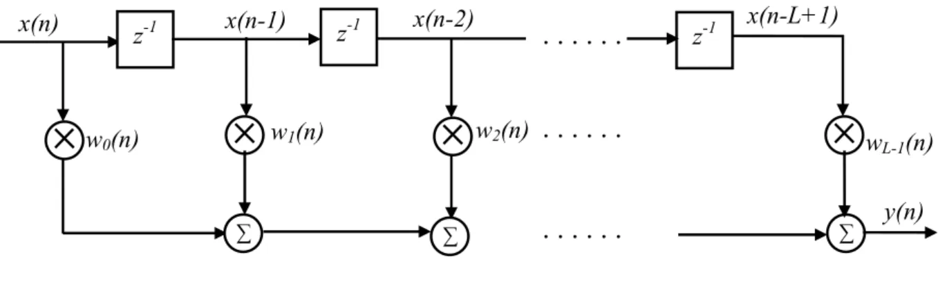
2.3. FILTER STRUCTURES
In general, any system with a finite number of parameters that affect how y(n) is computed
from x(n) could be used for the adaptive filter in Fig. 2.2.. Define the parameter or coefficient vector W(n)
W n( ) [ ( )= w n0 w n1( ) . . . wL-1( )]n T (2.2) where {wi (n)}, 0 < i < L - 1 are the L parameters of the system at time n. With this definition, we could define a general input-output relationship for the adaptive filter as
( ) ( ( ), ( - ), ( - 2), ..., ( - ), ( ), ( - ),..., ( - ))
y n = f W n y n l y n y n N x n x n l x n M l+ (2.3) where f ( ) represents any well-defined linear or nonlinear function and M and N are positive integers. Implicit in this definition is the fact that the filter is causal, such that future values of
( )
x n are not needed to compute. While non-causal filters can be handled in practice by suitably buffering or storing the input signal samples, we do not consider this possibility.
Although Equation (2.3) is the most general description of an adaptive filter structure, we are interested in determining the best linear relationship between the input and desired response signals for many problems. This relationship typically takes the form of a finite-impulse-response (FIR) or infinite-finite-impulse-response (IIR) filter. Figure2.3. shows the structure of a direct-form FIR filter, also known as a tapped-delay-line or transversal filter, where z-1 denotes the unit delay element and each wi (n) is a multiplicative gain within the system. In
this case, the parameters in W(n) correspond to the impulse response values of the filter at time n. We can write the output signal y(n) as
1 0 ( ) L i( ) ( ) i y n − w n x n i = =
∑
− (2.4)=W n X nT( ) ( ) (2.5) where X n( ) [ ( )= x n x n( - 1) ( - x n L + )]l Tdenotes the input signal vector and -T
denotes vector transpose. Note that this system requires L multiplies and L - 1 adds to implement and these computations are easily performed by a processor or circuit so long as L is not too large and the sampling period for the signals is not too short. It also requires a total of 2L memory locations to store the L input signal samples and the L coefficient values, respectively.
2.4. APPLICATION OF ADAPTIVE FILTERS.
Perhaps the most important driving forces behind the developments in adaptive filters
throughout their history have been the wide range of applications in which such systems can be used. We now discuss the forms of these applications in terms of more-general problem classes that describe the assumed relationship between d(n) and x(n). Our discussion illustrates the key issues in selecting an adaptive filter for a particular task.
2.4.1. Direct Modeling (System Identification)
In this type of modeling the adaptive model is kept parallel with the unknown plant. Modeling a single-input, single-output system is illustrated in Fig.2.4..Both the unknown system and adaptive filter are driven by the same input. The adaptive filter adjusts itself in such a way that its output is match with that of the unknown system. Upon convergence, the structure and parameter values of the adaptive system may or may not resemble those of unknown systems, but the input-output response relationship will match. In this sense, the adaptive system becomes a model of the unknown plant
wL-1(n) z-1 z-1 x(n) z-1
. . . .
. . .
. . .
∑ ∑ ∑ w0(n) w1(n) w2(n) y(n)Fig. 2.3. Structure of an FIR Filter x(n-2)
Unknown plant d(n) x(n) Σ y (n) e(n) + Adaptive model
Fig.2.4. Direct Modelling
Let d(n) and y(n) represent the output of the unknown system and adaptive model with x(n) as its input.
Here, the task of the adaptive filter is to accurately represent the signal d(n) at its output. If y(n) = d (n), then the adaptive filter has accurately modeled or identified the portion of the unknown system that is driven by x(n).
Since the model typically chosen for the adaptive filter is a linear filter, the practical goal of the adaptive filter is to determine the best linear model that describes the input-output relationship of the unknown system. Such a procedure makes the most sense when the unknown system is also a linear model of the same structure as the adaptive filter, as it is possible that y(n) = d(n) for some set of adaptive filter parameters. For ease of discussion, let the unknown system and the adaptive filter both be FIR filters, such that
( ) T ( ) ( ) OPT
d n =W n X n (2.6) where WOPT(n) is an optimum set of filter coefficients for the unknown system at time n. In
this problem formulation, the ideal adaptation procedure would adjust W(n) such that W(n) = WOPT (n) as n →∞. In practice, the adaptive filter can only adjust W(n) such that y(n) closely
approximates d(n) over time.
The system identification task is at the heart of numerous adaptive filtering applications. We list several of these applications here[2.3]
• Plant Identification
• Echo Cancellation for Long-Distance Transmission
• Acoustic Echo Cancellation
2.4.2. Inverse Modeling
We now consider the general problem of inverse modeling, as shown in Fig.2.5. In this diagram, a source signals s(n) is fed into a plant that produces the input signal x(n) for the adaptive filter. The output of the adaptive filter is subtracted from a desired response signal that is a delayed version of the source signal, such that
( ) ( - )
d n = s n Δ (2.7) where ∆ is a positive integer value. The goal of the adaptive filter is to adjust its characteristics such that the output signal is an accurate representation of the delayed source signal. plant d(n) s(n) Σ y (n) + Adaptive filter (inverse model) Σ delay x(n) + + Plant noise
Fig.2.5. Inverse Modelling
e(n)
2.5. GRADIENT BASED ADAPTIVE ALGORITHM
An adaptive algorithm is a procedure for adjusting the parameters of an adaptive filter to minimize a cost function chosen for the task at hand. In this section, we describe the general form of many adaptive FIR filtering algorithms and present a simple derivation of the LMS adaptive algorithm. In our discussion, we only consider an adaptive FIR filter structure, such that the output signal y(n) is given by (2.5). Such systems are currently more popular than adaptive IIR filters because
(1) The input-output stability of the FIR filter structure is guaranteed for any set of fixed coefficients, and
(2) The algorithms for adjusting the coefficients of FIR filters are simpler in general than those for adjusting the coefficients of IIR filters.
2.5.1. General Form of Adaptive FIR Algorithm
The general form of an adaptive FIR filtering algorithm is
W(n+1)=W(n)+μ(n)G(e(n),X(n),φ(n)) (2.8) where G(-) is a particular vector-valued nonlinear function, μ(n) is a step size parameter, e(n) and X(n) are the error signal and input signal vector, respectively, and
( )n
φ is a vector of states that store pertinent information about the characteristics of the input and error signals and/or the coefficients at previous time instants. In the simplest algorithms, φ( )n is not used, and the only information needed to adjust the coefficients at time n are the error signal, input signal vector, and step size.
The step size is so called because it determines the magnitude of the change or "step" that is taken by the algorithm in iteratively determining a useful coefficient vector. Much research effort has been spent characterizing the role that μ( )n plays in the performance of adaptive filters in terms of the statistical or frequency characteristics of the input and desired response signals. Often, success or failure of an adaptive filtering application depends on how the value of μ(n) is chosen or calculated to obtain the best performance from the adaptive filter.
2.5.2. The Mean-Squared Error Cost Function
The form of G(-) in (2.8) depends on the cost function chosen for the given adaptive filtering task. We now consider one particular cost function that yields a popular adaptive algorithm. Define the mean-squared error (MSE) cost function as
∫
∞ ∞ − = ( ) ( ( )) ( ) 2 1 ) (n e2 n p e n de n JMSE n (2.9) { ( )} 2 1E e2 n = (2.10) where pn(e(n)) represents the probability density function of the error at time n andE{-} is shorthand for the expectation integral on the right-hand side of (2.10). The MSE cost function is useful for adaptive FIR filters because
• the coefficient values obtained at this minimum are the ones that minimize the power in the error signal e(n), indicating that y(n) has approached d{n); and
• JMSE is a smooth function of each of the parameters in W(n), such that it is
differentiable with respect to each of the parameters in W(n).
The third point is important in that it enables us to determine both the optimum coefficient values given knowledge of the statistics of d(n) and x(n) as well as a simple iterative procedure for adjusting the parameters of an FIR filter.
2.5.3. The Wiener Solution.
For the FIR filter structure, the coefficient values in W(n) that minimize JMSE(n) are
well-defined if the statistics of the input and desired response signals are known. The formulation of this problem for continuous-time signals and the resulting solution was first derived by Wiener [2.5]. Hence, this optimum coefficient vector WMSE(n) is often
called the Wiener solution to the adaptive filtering problem. The extension of Wiener's analysis to the discrete-time case is attributed to Levinson [2.6]. To determine WMSE (n) we note that the function JMSE(n) in (2.10) is quadratic in the
parameters {wi(n)}, and the function is also differentiable. Thus, we can use a result
from optimization theory that states that the derivatives of a smooth cost function with respect to each of the parameters is zero at a minimizing point on the cost function
error surface. Thus, WMSE (n) can be found from the solution to the system of
equations 0 ) ( ) ( = ∂ ∂ n w n J i MSE ,0≤i≤ L−1 (2.11)
Taking derivatives of JMSE(n) in (2.10) we obtain
} ) ( ) ( ) ( { ) ( ) ( n w n e n e E n w n J i i MSE ∂ ∂ = ∂ ∂ (2.12) } ) ( ) ( ) ( { n w n y n e E i ∂ ∂ − = (2.13) =−E{e(n)x(n−i)} (2.14)
-1 0 - ( { ( ) ( - )} - { ( - ) ( - )} ( )) L j j E d n x n i E x n i x n j w n = =
∑
(2.15)where we have used the definitions of e(n) and of y(n) for the FIR filter structure in (2.1) and (2.5), respectively, to expand the last result in (2.15). By defining the matrix RXX(n)(autocorrelation matrix) and vector Pdx(n)(cross correlation matrix) as
{ ( ) ( )} ( ) { ( ). ( )} T XX dx R E X n X n and P n E d n X n = = (2.16)
respectively, we can combine (2.11) and (2.15) to obtain the system of equations in vector form as
RXX(n)WMSE(n)−Pdx(n)=0 (2.17) where 0 is the zero vector. Thus, so long as the matrix RXX(n) is invertible, the optimum Wiener solution vector for this problem is
) ( ) ( ) (n R 1 n P n WMSE = XX− dx
(2.18)
2.5.4. The Method of Steepest Descent
The method of steepest descent is a celebrated optimization procedure for minimizing the value of a cost function J(n) with respect to a set of adjustable parameters W(n). This procedure adjusts each parameter of the system according to
) ( ) ( ) ( ) ( ) 1 ( n w n J n n w n w i i i ∂ ∂ − = + μ (2.19)
In other words, the ith parameter of the system is altered according to the derivative of the cost function with respect to the ith parameter. Collecting these equations in vector form, we have
) ( ) ( ) ( ) ( ) 1 ( n W n J n n W n W ∂ ∂ − = + μ (2.20)
where ∂J(n)/∂W(n) is a vector of derivatives dJ(n)/dwi(n).
Substituting these results into (2.19) yields the update equation for W(n) as )) ( ) ( ) ( )( ( ) ( ) 1 (n W n n P n R nW n W + = +μ dx − XX (2.21)
However, this steepest descent procedure depends on the statistical quantities
E{d(n)x(n-i)} and E{x(n-i)x(n-j)} contained in Pdx(n) and Rxx(n), respectively. In
practice, we only have measurements of both d(n) and x(n) to be used within the adaptation procedure. While suitable estimates of the statistical quantities needed for (2.21) could be determined from the signals x(n) and d{n), we instead develop an approximate version of the method of steepest descent that depends on the signal values themselves. This procedure is known as the LMS(least mean square) algorithm.
2.6. LMS ALGORITHM
The cost function J(n) chosen for the steepest descent algorithm of (2.19) determines the coefficient solution obtained by the adaptive filter. If the MSE cost function in (2.10) is chosen, the resulting algorithm depends on the statistics of x(n) and d(n) because of the expectation operation that defines this cost function. Since we typically only have measurements of d(n) and of x(n) available to us, we substitute an alternative cost function that depends only on these measurements. One such cost function is the least-squares cost function given by
∑
(2.22) = − = n k T LS n k d k W n X k J 0 2 )) ( ) ( ) ( )( ( ) ( αwhere α(n) is a suitable weighting sequence for the terms within the summation. This cost function, however, is complicated by the fact that it requires numerous computations to calculate its value as well as its derivatives with respect to each
W(n), although efficient recursive methods for its minimization can be developed.
Alternatively, we can propose the simplified cost function JLMS(n)given by ) ( 2 1 ) (n e2 n JLMS = (2.23) This cost function can be thought of as an instantaneous estimate of the MSE cost function, as JMSE(n) = E{JLMS(n)}. Although it might not appear to be useful, the
resulting algorithm obtained when JLMS(n) is used for J(n) in (2.19) is extremely
useful for practical applications. Taking derivatives of JLMS(n) with respect to the
elements of W(n) and substituting the result into (2.19), we obtain the LMS adaptive algorithm given by
W(n+1)=W(n)+μ(n)e(n)X(n) (2.24) Equation (2.24) requires only multiplications and additions to implement. In fact,
the number and type of operations needed for the LMS algorithm is nearly the same as that of the FIR filter structure with fixed coefficient values, which is one of the reasons for the algorithm's popularity.
The behavior of the LMS algorithm has been widely studied, and numerous results concerning its adaptation characteristics under different situations have been developed. For now, we indicate its useful behavior by noting that the solution obtained by the LMS algorithm near its convergent point is related to the Wiener solution. In fact, analysis of the LMS algorithm under certain statistical assumptions about the input and desired response signals show that
{ ( )} ( )
lim
MSE n E W n W n →∞ = (2.25) when the Wiener solution WMSE (n) is a fixed vector. Moreover, the average behaviorof the LMS algorithm is quite similar to that of the steepest descent algorithm in (2.21) that depends explicitly on the statistics of the input and desired response signals. In effect, the iterative nature of the LMS coefficient updates is a form of time-averaging that smoothes the errors in the instantaneous gradient calculations to obtain a more reasonable estimate of the true gradient.
The problem is that gradient descent is a local optimization technique, which is limited because it is unable to converge to the global optimum on a multimodal error surface if the algorithm is not initialized in the basin of attraction of the global optimum.
Several modifications exist for gradient based algorithms in attempt to enable them to overcome local optima. One approach is to simply add a momentum term [2.3] to the gradient computation of the gradient descent algorithm to enable it to be more likely to escape from a local minimum. This approach is only likely to be successful when the error surface is relatively smooth with minor local minima, or some information can be inferred about the topology of the surface such that the additional gradient parameters can be assigned accordingly. Other approaches attempt to transform the error surface to eliminate or diminish the presence of local minima [2.16], which would ideally result in a unimodal error surface. The problem with these approaches is that the resulting minimum transformed error used to update the adaptive filter can be biased from the true minimum output error and the algorithm may not be able to converge to the desired minimum error
condition. These algorithms also tend to be complex, slow to converge, and may not be guaranteed to emerge from a local minimum. Some work has been done with regard to removing the bias of equation error LMS [2.7][2.8] and Steiglitz-McBride [2.9]adaptive IIR filters, which add further complexity with varying degrees of success.
Another approach [2.10], attempts to locate the global optimum by running several LMS algorithms in parallel, initialized with different initial coefficients. The notion is that a larger, concurrent sampling of the error surface will increase the likelihood that one process will be initialized in the global optimum valley. This technique does have potential, but it is inefficient and may still suffer the fate of a standard gradient technique in that it will be unable to locate the global optimum. By using a similar congregational scheme, but one in which information is collectively exchanged between estimates and intelligent randomization is introduced, structured stochastic algorithms are able to hill-climb out of local minima. This enables the algorithms to achieve better, more consistent results using a fewer number of total estimate.
2.7. SYSTEM IDENTIFICATION
System identification concerns with the determination of a system, on the basis of input output data samples. The identification task is to determine a suitable estimate of finite dimensional parameters which completely characterize the plant. The selection of the estimate is based on comparison between the actual output sample and a predicted value on the basis of input data up to that instant. An adaptive automaton is a system whose structure is alterable or adjustable in such a way that its behavior or performance improves through contact with its environment.
Depending upon input-output relation, the identification of systems can have two groups A. Static System Identification
In this type of identification the output at any instant depends upon the input at that instant. These systems are described by the algebraic equations. The system is essentially a memoryless one and mathematically it is represented as y(n) = f [x(n)] where y(n) is the output at the nth instant corresponding to the input x(n).
B. Dynamic System Identification
In this type of identification the output at any instant depends upon the input at that instant as well as the past inputs and outputs. Dynamic systems are described by the difference or differential equations. These systems have memory to store past values and mathematically
represented as y(n)=f [x(n), x(n-1),x(n-2)………..y(n-1),y(n-2),……] where y(n) is the output at the nth instant corresponding to the input x(n).
A system identification structure is shown in Fig.2.6. The model is placed parallel to the nonlinear plant and same input is given to the plant as well as the model. The impulse response of the linear segment of the plant is represented by h(n) which is followed by nonlinearity(NL) associated with it. White Gaussian noise q(n) is added with nonlinear output accounts for measurement noise. The desired output d(n) is compared with the estimated output y(n) of the identifier to generate the error e(n) which is used by some adaptive algorithm for updating the weights of the model. The training of the filter weights is continued until the error becomes minimum and does not decrease further. At this stage the correlation between input signal and error signal is minimum. Then the training is stopped and the weights are stored for testing. For testing purpose new samples are passed through both the plant and the model and their responses are compared.
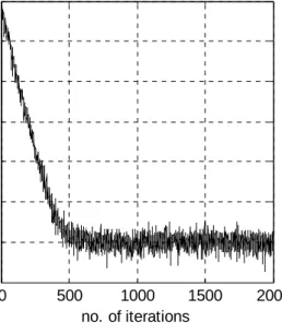
2.8. SIMULATION RESULTS
The performance of LMS algorithm is tested for both linear and nonlinear systems. For identification purpose a tap delay filter with three taps is used. The parameter of the linear
∑ Plant h(n) Update algorithm Model + N.L. Noise + _ y(n) d(n) x(n) e(n) a(n) b(n) q(n) Nonlinear plant
part of the plant is h(n)= [0.26 0.93 0.26].The different type of nonlinearity considered here are (I) b n( ) tanh( ( ))= a n (II) b n( )=a n( ) 0.2 ( ) 0.1 ( )+ a n2 − a n3 (III) b n( )=a n( ) 0.9 ( )− a n3 (IV) b n( )=a n( ) 0.2 ( ) 0.1 ( ) 0.5cos(+ a n2 − a n3 + πa n( )) (2.26)
For the simulation the initial parameters of the model taken as zeros. Gaussian noise of signal to noise ratio (SNR) 30dB was added which accounts for measurement noise. The input to the plant was taken from a uniformly distributed random signal over the interval [-0.5, 0.5] .The adaptation is continued for 2000 iterations which is ensembled over 50 iterations. After training filter weights remain fixed. For testing new 20 samples are generated and pass through the plant as well as model. The mean square error (MSE) and responses are plotted for the linear and nonlinear systems.
(i)For linear system:
0 500 1000 1500 2000 -35 -30 -25 -20 -15 -10 -5 0 no. of iterations MS E in d B MSE plot 0 5 10 15 20 -0.5 0 0.5 no. of samples re po ns es response plot actual lms (a) (b) Fig. 2.7. (a) MSE plot ,(b)response plot
(ii)For nonlinearity (I) 0 500 1000 1500 2000 -35 -30 -25 -20 -15 -10 -5 0 no. of iterations MS E in d B MSE plot 0 5 10 15 20 -0.5 0 0.5 no. of samples repo ns es response plot actual lms (a) (b) Fig. 2.8. (a) MSE plot ,(b)response plot
(iii)For nonlinearity (II)
0 500 1000 1500 2000 -30 -25 -20 -15 -10 -5 0 no. of iterations MS E in d B MSE plot 0 5 10 15 20 -0.5 0 0.5 no. of samples re po ns es response plot actual lms (a) (b) Fig. 2.9. (a) MSE plot ,(b)response plot
(iv)For nonlinearity (III) 0 500 1000 1500 2000 -25 -20 -15 -10 -5 0 no. of iterations MS E i n d B MSE plot 0 5 10 15 20 -0.4 -0.3 -0.2 -0.1 0 0.1 0.2 0.3 0.4 no. of samples re po ns e s response plot actual lms (a) (b) Fig. 2.10. (a) MSE plot ,(b)response plot
(v)For nonlinearity (IV)
0 500 1000 1500 2000 -4 -3 -2 -1 0 no. of iterations MS E in d B MSE plot 0 5 10 15 20 -0.6 -0.4 -0.2 0 0.2 0.4 0.6 0.8 no. of samples re po ns es response plot actual lms (a) (b) Fig. 2.11. (a) MSE plot ,(b)response plot
2.9. SUMMARY
Application of adaptive filter and two types of modeling is described in this chapter. System identification deals with direct modeling. The LMS algorithm is used for system identification purpose because of its simplicity. From Fig (2.7) to (2.11) it is observed that for linear system LMS algorithm based model gives best result. As the nonlinearity associated with the system goes on increasing the LMS based model response deviates from the actual response. Taking different types of nonlinearity the MSE and responses are plotted. From Fig.2.11 it is seen that the actual response and the LMS based model response do not match anywhere. From this we conclude that LMS based models are best for linear systems.
Chapter
3
3. SYSTEM IDENTIFICATION USING ANN
3.1. INTRODUCTION
Because of nonlinear signal processing and learning capability, Artificial Neural Networks (ANN’s) have become a powerful tool for many complex applications including functional approximation, nonlinear system identification and control, pattern recognition and classification, and optimization. The ANN’s are capable of generating complex mapping between the input and the output space and thus, arbitrarily complex nonlinear decision boundaries can be formed by these networks. An artificial neuron basically consists of a computing element that performs the weighted sum of the input signal and the connecting weight. The sum is added with the bias or threshold and the resultant signal is then passed through a non-linear element of tanh(.) type. Each neuron is associated with three parameters whose learning can be adjusted; these are the connecting weights, the bias and the slope of the non-linear function. For the structural point of view a neural network(NN) may be single layer or it may be multi-layer. In multi-layer structure, there is one or many artificial neurons in each layer and for a practical case there may be a number of layers. Each neuron of the one layer is connected to each and every neuron of the next layer.
A neural network is a massively parallel distributed processor made up of simple processing unit, which has a natural propensity for storing experimental knowledge and making it available for use. It resembles the brain in two types
1. Knowledge is acquired by the network from its environment through a learning process.
2. Interneuron connection strengths, known as synaptic weights, are used to store the acquired knowledge.
Artificial Neural Networks (ANN) has emerged as a powerful learning technique to perform complex tasks in highly nonlinear dynamic environments. Some of the prime advantages of using ANN models are their ability to learn based on optimization of an appropriate error function and their excellent performance for approximation of nonlinear function [3.1]. At present, most of the work on system identification using neural networks are based on multilayer feed forward neural networks with back propagation learning or more efficient variations of this algorithm [3.2] ,[3.3].On the otherhand the Functional link ANN(FLANN) originally proposed by Pao[3.4] is a single layer structure with functionally mapped inputs. The performance of FLANN for system identification of nonlinear systems
has been reported [3.5] in the literature. Patra and Kot [3.6] have used Chebyschev expansions for nonlinear system identification and have shown that the identification performance is better than that offered by the multilayer ANN (MLANN) model. Wang and Chen [3.7] have presented a fully automated recurrent neural network (FARNN) that is capable of self-structuring its network in a minimal representation with satisfactory performance for unknown dynamic system identification and control.
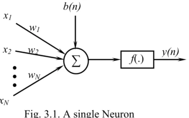
3.2. SINGLE NEURON STRUCTURE
In 1958, Rosenblatt demonstrated some practical applications using the perceptron [3.8].
The perceptron is a single level connection of McCulloch-Pitts neurons sometimes called single-layer feed forward networks. The network is capable of linearly separating the input vectors into pattern of classes by a hyper plane. A linear associative memory is an example of a single-layer neural network. In such an application, the network associates an output pattern (vector) with an input pattern (vector), and information is stored in the network by virtue of modifications made to the synaptic weights of the network.
The structure of a single neuron is presented in Fig. 3.1.An artificial neuron involves the computation of the weighted sum of inputs and threshold [3.9, 3.10]. The resultant signal is then passed through a non-linear activation function. The output of the neuron may be represented as,
( )
( ) ( )
(3.1) 1 ( ) N j j j y n f w n x n b n = ⎡ ⎤ = ⎢ ⎣∑
⎦∑
f(.)• • •
x1 x2 xN b(n) y(n)Fig. 3.1. A single Neuron w2
w1
wN
+ ⎥
Where b(n) = threshold to the neuron is called as bias.
3.2.1. Activation Functions and Bias.
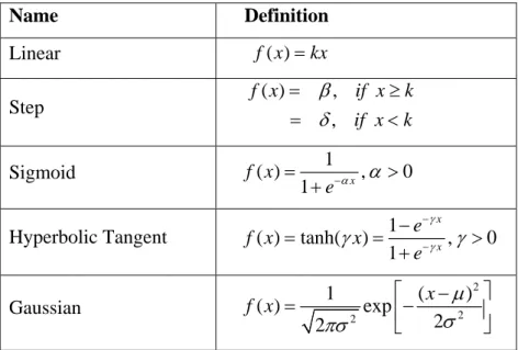
The perceptron internal sum of the inputs is passed through an activation function, which can be any monotonic function. Linear functions can be used but these will not contribute to a non-linear transformation within a layered structure, which defeats the purpose of using a neural filter implementation. A function that limits the amplitude range and limits the output strength of each perceptron of a layered network to a defined range in a non-linear manner will contribute to a nonlinear transformation. There are many forms of activation functions, which are selected according to the specific problem. All the neural network architectures employ the activation function [3.1, 3.8] which defines as the output of a neuron in terms of the activity level at its input (ranges from -1 to 1 or 0 to 1). Table 3.1 summarizes the basic types of activation functions. The most practical activation functions are the sigmoid and the hyperbolic tangent functions. This is because they are differentiable.
The bias gives the network an extra variable and the networks with bias are more powerful than those of without bias. The neuron without a bias always gives a net input of zero to the activation function when the network inputs are zero. This may not be desirable and can be avoided by the use of a bias.
Table 3.1 COMMON ACTIVATION FUNCTIONS
Name Definition Linear f x( )=kx Step ( ) , , f x if x if x k k β δ = ≥ = < Sigmoid ( ) 1 , 0 1 x f x e−α α = > +
Hyperbolic Tangent ( ) tanh( ) 1 , 0
1 x x e f x x e γ γ γ − −− γ = = > + Gaussian 2 2 2 1 ( ( ) exp 2 2 x f x μ σ πσ ) ⎡ − ⎤ = ⎢− ⎥ ⎣ ⎦ 3.2.2 Learning Processes
The property that is of primary significance for a neural network is that the ability of the network to learn from its environment, and to improve its performance through learning. The improvement in performance takes place over time in accordance with some prescribed
measure. A neural network learns about its environment through an interactive process of adjustments applied to its synaptic weights and bias levels. Ideally, the network becomes more knowledgeable about its environment after each iteration of learning process. Hence we define learning as:
“It is a process by which the free parameters of a neural network are adapted through a process of stimulation by the environment in which the network is embedded.”
The processes used are classified into two categories as described in [3.1]: (A) Supervised Learning (Learning With a Teacher)
(B) Unsupervised Learning (Learning Without a Teacher) (A) Supervised Learning:
We may think of the teacher as having knowledge of the environment, with that knowledge being represented by a set of input-output examples. The environment is, however unknown to neural network of interest. Suppose now the teacher and the neural network are both exposed to a training vector, by virtue of built-in knowledge, the teacher is able to provide the neural network with a desired response for that training vector. Hence the desired response represents the optimum action to be performed by the neural network. The network parameters such as the weights and the thresholds are chosen arbitrarily and are updated during the training procedure to minimize the difference between the desired and the estimated signal. This updation is carried out iteratively in a step-by-step procedure with the aim of eventually making the neural network emulate the teacher. In this way knowledge of the environment available to the teacher is transferred to the neural network. When this condition is reached, we may then dispense with the teacher and let the neural network deal with the environment completely by itself. This is the form of supervised learning.
The update equations for weights are derived as LMS [3.11]:
(
1)
( ) ( j j w n+ =w n + Δμ w nj ) (3.2) ( ) j w nΔ is the change in wj in nth iteration.
(B) Unsupervised Learning:
In unsupervised learning or self-supervised learning there is no teacher to over-see the learning process, rather provision is made for a task independent measure of the quantity of representation that the network is required to learn, and the free parameters of the network are optimized with respect to that measure. Once the network has become turned to the statistical regularities of the input data, it develops the ability to form the internal representations for
encoding features of the input and thereby to create new classes automatically. In this learning the weights and biases are updated in response to network input only. There are no desired outputs available. Most of these algorithms perform some kind of clustering operation. They learn to categorize the input patterns into some classes.
3.3. MULTILAYER PERCEPTRON
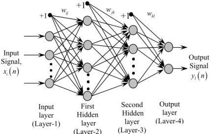
In the multilayer neural network or multilayer perceptron (MLP), the input signal propagates through the network in a forward direction, on a layer-by-layer basis. This network has been applied successfully to solve some difficult and diverse problems by training in a supervised manner with a highly popular algorithm known as the error back-propagation algorithm [3.1,3.9]. The scheme of MLP using four layers is shown in Fig.3.2.
( )
ix n represent the input to the network, fj and fk represent the output of the two hidden layers and y n l
( )
represents the output of the final layer of the neural network. The connecting weights between the input to the first hidden layer, first to second hidden layer and the second hidden layer to the output layers are represented byrespectively.
, and
ij jk kl
w w w
Fig. 3.2 Structure of multilayer perceptron
•••
•••
•••
First Hidden layer (Layer-2) Input layer (Layer-1) Output layer (Layer-4) Input Signal,( )
i x n Output Signal( )
l y n Second Hidden layer (Layer-3) +1 wij +1 wjk +1 kl wIf P1 is the number of neurons in the first hidden layer, each element of the output vector of
first hidden layer may be calculated as,
( )
1 j j ij i j i N f ϕ w x n b = ⎡ ⎤ = ⎢ + ⎥ ⎣∑
⎦i=1, 2,3,... ,N j=1, 2,3,...P1 (3.3)where bj is the threshold to the neurons of the first hidden layer, N is the no. of inputs and
( )
.ϕ is the nonlinear activation function in the first hidden layer chosen from the Table 3.1. The time index n has been dropped to make the equations simpler. Let P2 be the number of
neurons in the second hidden layer. The output of this layer is represented as, fk and may be
written as 1 1 k k jk j k j P f ϕ w f b = ⎡ ⎤ = ⎢ ⎣
∑
+ ⎥⎦ P l + ⎥ , k=1, 2, 3, …, P2 (3.4)where, is the threshold to the neurons of the second hidden layer. The output of the final output layer can be calculated as
k b
( )
2 1 l l kl k k y n ϕ w f b = ⎡ ⎤ = ⎢ ⎣∑
⎦, l=1, 2, 3, … , P3 (3.5)where, αl is the threshold to the neuron of the final layer and P3 is the no. of neurons in the
output layer. The output of the MLP may be expressed as
( )
2 1( )
1 1 1 N l n kl k jk j ij i j k k j i y n ϕ w ϕ w ϕ w x n b b b = = = ⎡ ⎛ ⎧ ⎫ ⎞ ⎤ = ⎢ ⎜ ⎨ ⎬ ⎥ ⎩ ⎭ ⎢ ⎝ ⎠ ⎥ ⎣∑
∑
∑
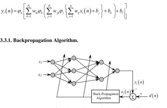
⎦ P P l + + ⎟+ (3.6) 3.3.1. Backpropagation Algorithm.Fig. 3.3 Neural network using BP algorithm Σ Back-Propagation Algorithm x1 x2
( )
l y n( )
d n( )
l e n - +An MLP network with 2-3-2-1 neurons (2, 3, 2 and 1 denote the number of neurons in the input layer, the first hidden layer, the second hidden layer and the output layer respectively) with the back-propagation (BP) learning algorithm, is depicted in Fig.3.3. The parameters of
the neural network can be updated in both sequential and batch mode of operation. In BP algorithm, initially the weights and the thresholds are initialized as very small random values. The intermediate and the final outputs of the MLP are calculated by using (3.3), (3.4.), and (3.5.) respectively.
(
The final output y nl
)
at the output of neuron l, is compared with the desired outputd n( )
and the resulting error signal( )
l
l
e n is obtained as
e nl
( )
=d n( )
−y n( )
(3.7)The instantaneous value of the total error energy is obtained by summing all error signals over all neurons in the output layer, that is
( )
( )
3 2 1 1 2 l l n e ξ = =∑
P n (3.8)where P3 is the no. of neurons in the output layer.
This error signal is used to update the weights and thresholds of the hidden layers as well as the output layer. The reflected error components at each of the hidden layers is computed using the errors of the last layer and the connecting weights between the hidden and the last layer and error obtained at this stage is used to update the weights between the input and the hidden layer. The thresholds are also updated in a similar manner as that of the corresponding connecting weights. The weights and the thresholds are updated in an iterative method until the error signal becomes minimum. For measuring the degree of matching, the Mean Square Error (MSE) is taken as a performance measurement.
The updated weights are,
w nkl
(
+ =1)
w nkl( )
+ Δw nkl( )
(3.9) wjk(
n+ =1)
wjk( )
n + Δwjk( )
n (3.10) w nij(
+ =1)
w nij( )
+ Δw nij( )
(3.11) where, Δw nkl( )
,Δwjk( )
n and Δw nij( )
are the change in weights of the second hiddenlayer-to-output layer, first hidden layer-to-second hidden layer and input layer-to-first hidden layer respectively. That is,
( )
( )
( )
( )
( )
( )
( )
2 1 2 l kl kl kl P l kl k l k d n dy n w n e n dw n dw n e n w f f ξ μ μ μ ϕ α = Δ = − = ⎡ ⎤ ′ = ⎢ + ⎥ ⎣∑
⎦ k (3.12)Where, μ is the convergence coefficient (0≤ ≤μ 1). Similarly the can
be computed [3.1].
( )
( )
(
)
( )
l( )
(
)
( )
k( )
j( )
( )
( )
( )
and Δwjk n Δw nijThe thresholds of each layer can be updated in a similar manner, i.e.
b nl + =1 b nl + Δb n (3.13)
b nk + =1 b nk + Δb n (3.14)
b nj
(
+ =1)
b nj( )
+ Δb n( )
(3.15)where, are the change in thresholds of the output, hidden and
input layer respectively. The change in threshold is represented as,
, and l k j b n b n b n Δ Δ Δ
( )
( )
( ) ( )
( )
( )
2 1 2 l l l P l kl k l k d n dy n b n e n db n db n e n w f b ξ μ μ μ ϕ = Δ = − = ⎡ ⎤ ′ = ⎢ + ⎥ ⎣∑
⎦ l (3.16)3.4. FUNCTIONAL LINK ANN
Pao originally proposed FLANN and it is a novel single layer ANN structure capable of forming arbitrarily complex decision regions by generating nonlinear decision boundaries [3.4]. Here, the initial representation of a pattern is enhanced by using nonlinear function and thus the pattern dimension space is increased. The functional link acts on an element of a pattern or entire pattern itself by generating a set of linearly independent function and then evaluates these functions with the pattern as the argument. Hence separation of the patterns becomes possible in the enhanced space. The use of FLANN not only increases the learning rate but also has less computational complexity [3.13]. Pao et al [3.12] have investigated the learning and generalization characteristics of a random vector FLANN and compared with those attainable with MLP structure trained with back propagation algorithm by taking few functional approximation problems. A FLANN structure with two inputs is shown in Fig. 3.4.