Preprint typeset in JHEP style - PAPER VERSION Revised May 6, 2011
An Introduction to String Theory
Kevin Wray
Abstract: This set of notes is based on the course “Introduction to String Theory”
which was taught by Prof. Kostas Skenderis in the spring of 2009 at the University of Amsterdam. We have also drawn on some ideas from the books String Theory and
M-Theory (Becker, Becker and Schwarz), Introduction to String Theory (Polchinski),
String Theory in a Nutshell (McMahon) andSuperstring Theory (Green, Schwarz and Witten), along with the lecture notes of David Tong, sometimes word-for-word.
Contents
1. Introduction/Overview 5
1.1 Motivation for String Theory 5
1.2 What is String Theory 8
1.2.1 Types of String Theories 8
1.3 Outline of the Manuscript 9
2. The Bosonic String Action 11
2.1 Classical Action for Point Particles 11
2.2 Classical Action for Relativistic Point Particles 12
2.2.1 Reparametrization Invariance of ˜S0 16
2.2.2 Canonical Momenta 18
2.2.3 Varying ˜S0 in an Arbitrary Background (Geodesic Equation) 19
2.3 Generalization to p-Branes 19
2.3.1 The String Action 20
2.4 Exercises 24
3. Symmetries and Field Equations of the Bosonic String 26 3.1 Global Symmetries of the Bosonic String Theory Worldsheet 26 3.2 Local Symmetries of the Bosonic String Theory Worldsheet 30
3.3 Field Equations for the Polyakov Action 33
3.4 Solving the Field Equations 36
3.5 Exercises 42
4. Symmetries (Revisited) and Canonical Quantization 45
4.1 Noether’s Method for Generating Conserved Quantities 45
4.2 The Hamiltonian and Energy-Momentum Tensor 48
4.3 Classical Mass Formula for a Bosonic String 51
4.4 Witt Algebra (Classical Virasoro Algebra) 52
4.5 Canonical Quantization of the Bosonic String 54
4.6 Virasoro Algebra 56
4.7 Physical States 58
5. Removing Ghost States and Light-Cone Quantization 64
5.1 Spurious States 65
5.2 Removing the Negative Norm Physical States 68
5.3 Light-Cone Gauge Quantization of the Bosonic String 71
5.3.1 Mass-Shell Condition (Open Bosonic String) 74
5.3.2 Mass Spectrum (Open Bosonic String) 75
5.3.3 Analysis of the Mass Spectrum 77
5.4 Exercises 79
6. Introduction to Conformal Field Theory 80
6.1 Conformal Group in d Dimensions 80
6.2 Conformal Algebra in 2 Dimensions 83
6.3 (Global) Conformal Group in 2 Dimensions 85
6.4 Conformal Field Theories in d Dimensions 86
6.4.1 Constraints of Conformal Invariance in d Dimensions 87
6.5 Conformal Field Theories in 2 Dimensions 89
6.5.1 Constraints of Conformal Invariance in 2 Dimensions 90
6.6 Role of Conformal Field Theories in String Theory 92
6.7 Exercises 94
7. Radial Quantization and Operator Product Expansions 95
7.1 Radial Quantization 95
7.2 Conserved Currents and Symmetry Generators 96
7.3 Operator Product Expansion (OPE) 102
7.4 Exercises 105
8. OPE Redux, the Virasoro Algebra and Physical States 107
8.1 The Free Massless Bosonic Field 107
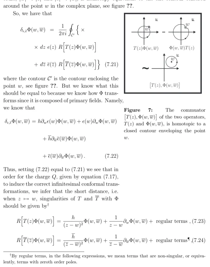
8.2 Charges of the Conformal Symmetry Current 115
8.3 Representation Theory of the Virasoro Algebra 119
8.4 Conformal Ward Identities 124
8.5 Exercises 127
9. BRST Quantization of the Bosonic String 129
9.1 BRST Quantization in General 129
9.1.1 BRST Quantization: A Primer 130
9.1.2 BRST Ward Identities 135
9.1.3 BRST Cohomology and Physical States 136
9.2.1 The Ghost CFT 146
9.2.2 BRST Current and Charge 151
9.2.3 Vacuum of the BRST Quantized String Theory 152
9.2.4 Ghost Current and Charge 154
9.3 Exercises 156
10. Scattering in String Theory 159
10.1 Vertex Operators 159
10.2 Exercises 160
11. Supersymmetric String Theories (Superstrings) 162
11.1 Ramond-Neveu-Schwarz Strings 163
11.2 Global Worldsheet Supersymmetry 166
11.3 Supercurrent and the Super-Virasoro Constraints 168
11.4 Boundary Conditions and Mode Expansions 172
11.4.1 Open RNS Strings 173
11.4.2 Closed RNS Strings 174
11.5 Canonical Quantization of the RNS Superstring Theory 175
11.5.1 R-Sector Ground State VS. NS-Sector Ground State 176 11.5.2 Super-Virasoro Generators (Open Strings) and Physical States 177
11.5.3 Physical State Conditions 180
11.5.4 Removing the Ghost States 181
11.6 Light-Cone Quantization 183
11.6.1 Open RNS String Mass Spectrum 184
11.6.2 GSO Projection 187
11.6.3 Closed RNS String Spectrum 190
11.7 Exercises 193
12. T-Dualities and Dp-Branes 197
12.1 T-Duality and Closed Bosonic Strings 197
12.1.1 Mode Expansion for the Compactified Dimension 199
12.1.2 Mass Formula 200
12.1.3 T-Duality of the Bosonic String 201
12.2 T-Duality and Open Strings 203
12.2.1 Mass Spectrum of Open Strings on Dp-Branes 206
12.3 Branes in Type II Superstring Theory 209
12.4 Dirac-Born-Infeld (DBI) Action 212
13. Effective Actions, Dualities, and M-Theory 216
13.1 Low Energy Effective Actions 216
13.1.1 Conformal Invariance of Sσ and the Einstein Equations 217
13.1.2 Other Couplings of the String 220
13.1.3 Low Energy Effective Action for the Bosonic String Theory 223 13.1.4 Low Energy Effective Action for the Superstring Theories 227
13.2 T-Duality on a Curved Background 229
13.3 S-Duality on the Type IIB Superstring Theories 233
13.3.1 Brane Solutions of Type IIB SUGRA 234
13.3.2 Action of the Brane Solutions Under the Duality Maps 236
13.4 M-Theory 239
13.5 Exercises 243
14. Black Holes in String Theory and the AdS/CFT Correspondence 245
14.1 Black Holes 245
14.1.1 Classical Theory of Black Holes 246
14.1.2 Quantum Theory of Black Holes 248
14.2 Black Holes in String Theory 251
14.2.1 Five-Dimensional Extremal Black Holes 252
14.3 Holographic Principle 255
14.3.1 The AdS/CFT Correspondence 255
A. Residue Theorem 260
B. Wick’s Theorem 261
1. Introduction/Overview
1.1 Motivation for String Theory
Presently we understand that physics can be described by four forces: gravity, elec-tromagnetism, the weak force, responsible for beta decays and the strong force which binds quarks into protons and neutrons. We, that is most physicists, believe that we understand all of these forces except for gravity. Here we use the word “understand” loosely, in the sense that we know what the Lagrangian is which describes how these forces induce dynamics on matter, and at least in principle we know how to calculate using these Lagrangians to make well defined predictions. But gravity we only under-stand partially. Clearly we underunder-stand gravity classically (meaning in the~= 0 limit).
As long as we dont ask questions about how gravity behaves at very short distances (we will call the relevant breakdown distance the Planck scale) we have no problems calculating and making predictions for gravitational interactions. Sometimes it is said that we don’t understand how to fuse quantum mechanics and GR. This statement is really incorrect, though for “NY times purposes”, it’s fine. In fact we understand perfectly well how to include quantum mechanical effects into gravity, as long we we dont ask questions about whats going on at distances, less than the Planck length. This is not true for the other forces. That is, for the other forces we know how to include quantum effects, at all distance scales.
So, while we have a quantum mechanical understanding of gravity, we don’t have a complete theory of quantum gravity. The sad part about this is that all the really interesting questions we want to ask about gravity, e.g. what’s the “big bang”, what happens at the singularity of black hole, are left unanswered. What is it, exactly, that goes wrong with gravity at scales shorter than the Planck length? The answer is, it is not “renormalizable”. What does “renormalizable” mean? This is really a technical question which needs to be discussed within the context of quantum field theory, but we can gain a very simple intuitive understanding from classical electromagnetism. So, to begin, consider an electron in isolation. The total energy of the electron is given by
ET ∼mˆ + Z d3x|E~|2 ∼mˆ + 4π Z r2dre 2 r4. (1.1)
Now, this integral diverges at the lower endpoint of r = 0. We can reconcile this divergence by cutting it off at some scale Λ and when were done well see if can take the limit where the cut-off goes to zero. So our results for the total energy of an electron is now given by
ET ∼mˆ +Ce 2
Clearly the second term dominates in the limit we are interested in. So apparently even classical electrodynamics is sick. Well not really, the point is that weve been rather sloppy. When we write ˆm what do we mean? Naively we mean what we would call the mass of the electron which we could measure say, by looking at the deflection of a moving electron in a magnetic field. But we dont measure ˆm, we measure ET, that is the inertial mass should include the electromagnetic self-energy. Thus what really happens is that the physical mass m is given by the sum of the bare mass ˆm and the electrons field energy. This means that the “bare” mass is “infinite” in the limit were interested in. Note that we must make a measurement to fix the bare mass. We can not predict the electron mass.
It also means that the bare mass must cancel the field energy to many digits. That is we have two huge numbers which cancel each other extremely precisely! To understand this better, note that it is natural to assume that the cut-off should be, by dimensional analysis, the Planck length (note: this is just a guess). Which in turn means that the self field energy is of order the Planck mass. So the bare mass must have a value which cancels the field energy to within at the level of the twenty second digit! Is this some sort of miracle? This cancellation is sometimes referred to as a “hierarchy problem”. This process of absorbing divergences in masses or couplings (an analogous argument can be made for the chargee) is called “renormalization”.
Now what happens with gravity (GR)? What goes wrong with this type of renor-malization procedure? The answer is nothing really. In fact, as mentioned above we can calculate quantum corrections to gravity quite well as long as we are at energies below the Planck mass. The problem is that when we study processes at energies of order the Planck mass we need more and more parameters to absorb the infinities that occur in the theory. In fact we need an infinite number of parameters to renormalize the theory at these scales. Remember that for each parameter that gets renormalized we must make a measurement! So GR is a pretty useless theory at these energies.
How does string theory solve this particular problem? The answer is quite simple. Because the electron (now a string) has finite extent lp, the divergent integral is cut-off at r = lp, literally, not just in the sketchy way we wrote above using dimensional analysis. We now have no need to introduce new parameters to absorb divergences since there really are none. Have we really solved anything aside from making the energy mathematically more palatable? The answer is yes, because the electron mass as well as all other parameters are now a prediction (at least in principle, a pipe dream perhaps)! String theory has only one unknown parameter, which corresponds to the string length, which presumably is of orderlp, but can be fixed by the one and only one
measurement that string theory necessitates before it can be used to make predictions. It would seem, however, that we have not solved the hierarchy problem. String
theory would seem to predict that the electron mass is huge, of order of the inverse length of the string, unless there is some tiny number which sits out in front of the integral. It turns out that string theory can do more than just cut off the integral, it can also add an additional integral which cancels off a large chunk of the first integral, leaving a more realistic result for the electron mass. This cancellation is a consequence of “supersymmetry” which, as it turns out, is necessary in some form for string theory to be mathematically consistent.
So by working with objects of finite extent, we accomplish two things. First off, all of our integrals are finite, and in principle, if string theory were completely understood, we would only need one measurement to make predictions for gravitational interactions at arbitrary distances. But also we gain enormous predictive power (at least in principle, its not quite so simple as we shall see). Indeed in the standard model of particle physics, which correctly describes all interactions at least to energies of order 200 GeV, there are 23 free parameters which need to be fixed by experiment, just as the electron mass does. String theory, however, has only one such parameter in its Lagrangian, the string length‡! Never forget that physics is a predictive science. The less descriptive and the
more predictive our theory is, the better. In that sense, string theory has been a holy grail. We have a Lagrangian with one parameter which is fixed by experiment, and then you are done. You have a theory of everything! You could in principle explain all possible physical phenomena. To say that this a a dramatic simplification would be an understatement, but in principle at least it is correct. This opens a philosophical pandoras’ box which should be discussed late at night with friends.
But wait there is more! Particle physics tells us that there a huge number of “elementary particles”. Elementary particles can be split into two categories, “matter” and “force carriers”. These names are misleading and should only be understood as sounds which we utter to denote a set. The matter set is composed of six quarks u, d, s, c, b, t (up, down, strange, charm, bottom, top) while the force carriers are the photon the “electroweak bosons”, Z, W±, the gravitong and eight gluons responsible
for the strong force. There is the also the socalled “Higgs boson” for which we only have indirect evidence at this point. So, in particle physics, we have a Lagrangian which sums over all particle types and distinguishes between matter and force carriers in some way. This is a rather unpleasant situation. If we had a theory of everything all the particles and forces should be unified in some way so that we could write down ‡A warning, this is misleading because to describe a theory we need to know more than just the
Lagrangian, we also need to know the ground state, of which there can be many. Perhaps you have heard of the “string theory landscape”? What people are referring to is the landscape of possible ground states, or equivalently “vacau”. There are people that are presently trying to enumerate the ground states of string theory.
a Lagrangian for a “master entity”, and the particles mentioned would then just be different manifestations of this underlying entity. This is exactly what string theory does! The underlying entity is the string, and different excitations of the string represent different particles. Furthermore, force unification is built in as well. This is clearly a very enticing scenario.
With all this said, one should keep in mind that string theory is in some sense only in its infancy, and, as such, is nowhere near answering all the questions we hoped it would, especially regarding what happens at singularities, though it has certainly led to interesting mathematics (4-manifolds, knot theory....). It can also be said that it has taught us much about the subject of strongly coupled quantum field theories via dualities. There are those who believe that string theory in the end will either have nothing to do with nature, or will never be testable, and as such will always be relegated to be mathematics or philosophy. But, it is hard not to be awed by string theory’s mathematical elegance. Indeed, the more one learns about its beauty the more one falls under its spell. To some it has become almost a religion. So, as a professor once said: “Be careful, and always remember to keep your feet on the ground lest you be swept away by the siren that is the string”.
1.2 What is String Theory
Well, the answer to this question will be given
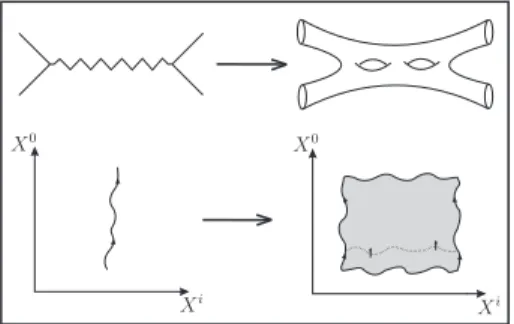
Figure 1: In string theory, Feyn-man diagrams are replaced by sur-faces and worldlines are replaced by worldsheets.
by the entire manuscript. In the meantime, roughly speaking, string theory replaces point particles by strings, which can be either open or closed (de-pends on the particular type of particle that is be-ing replaced by the strbe-ing), whose length, or strbe-ing length (denoted ls), is approximately 10−33cm.
Also, in string theory, one replaces Feynman dia-grams by surfaces, and wordlines become world-sheets.
1.2.1 Types of String Theories
The first type of string theory that will be discussed in these notes is that of bosonic string theory, where the strings correspond only to bosons. This theory, as will be shown later on, requires 26 dimensions for its spacetime.
In the mid-80’s it was found that there are 5 other consistent string theories (which include fermions):
• Type II A • Type II B
• Heterotic SO(32) • Heterotic E8×E8 .
All of these theories use supersymmetry, which is a symmetry that relates elementary particles of one type of spin to another particle that differs by a half unit of spin. These two partners are called superpartners. Thus, for every boson there exists its superpartner fermion and vice versa.
For these string theories to be physically consistent they require 10 dimensions for spacetime. However, our world, as we believe, is only 4 dimensional and so one is forced to assume that these extra 6 dimensions are extremely small. Even though these extra dimensions are small we still must consider that they can affect the interactions that are taking place.
It turns out that one can show, non-perturbatively, that all 5 theories are part of the same theory, related to each other throughdualities.
Finally, note that each of these theories can be extended toDdimensional objects, calledD-branes. Note here that D≤10 because it would make no sense to speak of a 15 dimensional object living in a 10 dimensional spacetime.
1.3 Outline of the Manuscript
We begin we a discussion of the bosonic string theory. Although this type of string theory is not very realistic, one can still get a solid grasp for the type of analysis that goes on in string theory. After we have defined the bosonic string action, or Polyakov action, we will then proceed to construct invariants, or symmetries, for this action. Using Noether’s theorem we will then find the conserved quantities of the theory, namely the stress energy tensor and Hamiltonian. We then quantize the bosonic string in the usual canonical fashion and calculate its mass spectrum. This, as will be shown, leads to inconsistencies with quantum physics since the mass spectrum of the bosonic string harbors ghost states - states with negative norm. However, the good news is that we can remove these ghost states at the cost of fixing the spacetime, in which the string propagates, dimension at 26. We then proceed to quantize the string theory in a different way known as light-cone gauge quantization.
The next stop in the tour is conformal field theory. We begin with an overview of the conformal group ind dimensions and then quickly restrict to the case ofd = 2. Then conformal field theories are defined and we look at the simplifications come with
a theory that is invariant under conformal transformations. This leads us directly into radial quantization and the notion of an operator product expansion (OPE) of two operators. We end the discussion of conformal field theories by showing how the charges (or generators) of the conformal symmetry are isomorphic to the Virasor algebra. With this we are done with the standard introduction to string theory and in the remaining chapters we cover developements.
The developements include scattering theory, BRST quantization and BRST coho-mology theory along with RNS superstring theories, dualities and D-branes, effective actions andM-theory and then finally matrix theory.
2. The Bosonic String Action
A string is a special case of ap-brane, where ap-brane is apdimensional object moving through a D(D≥p) dimensional spacetime. For example:
• a 0-brane is a point particle, • a 1-brane is a string,
• a 2-brane is a membrane .
Before looking at strings, let’s review the classical theory of 0-branes, i.e. point particles.
2.1 Classical Action for Point Particles
In classical physics, the evolution of a theory is described by its field equations. Suppose we have a non-relativistic point particle, then the field equations forX(t), i.e. Newton’s lawmX¨(t) =−∂V(X(t))/∂X(t), follow from extremizing the action, which is given by
S=
Z
dtL, (2.1)
whereL=T −V = 12mX˙(t)2 −V(X(t)). We have, by setting the variation ofS with
respect of the field X(t) equal to zero, 0 = δS =m Z dt1 2(2 ˙X)δX˙ − Z dt∂V ∂XδX =−m Z dtXδX¨ + boundary terms | {z } take = 0 − Z dt∂V ∂XδX =− Z dt mX¨ + ∂V ∂X δX ,
where in the third line we integrated the first term by parts. Since this must hold for allδX, we have that
mX¨(t) =−∂V(X(t))
∂X(t) , (2.2)
which are the equations of motion (or field equations) for the field X(t). These equa-tions describe the path taken by a point particle as it moves through Galilean spacetime (remember non-relativistic). Now we will generalize this to include relativistic point particles.
2.2 Classical Action for Relativistic Point Particles
For a relativistic point particle moving through aDdimensional spacetime, the classical motion is given by geodesics on the spacetime (since here we are no longer assuming a Euclidean spacetime and therefore we must generalize the notion of a straight line path). The relativistic action is given by the integral of the infinitesimal invariant length,ds, of the particle’s path, i.e.
S0 =−α
Z
ds, (2.3)
where α is a constant, and we have also chosen units in such a way that c = ~ = 1.
In order to find the equations that govern the geodesic taken by a relativistic particle we, once again, set the variation of the, now relativistic, action equal to zero. Thus, the classical motion of a relativistic point particle is the path which extremizes the invariant distance, whether it minimizes or maximizes ds depends on how one chooses to parametrize the path.
Now, in order forS0 to be dimensionless, we must have thatαhas units of Length−1
which means, in our chosen units, that α is proportional to the mass of the particle and we can, without loss of generality, take this constant of proportionality to be unity. Also, we choose to parameterize the path taken by a particle in such a way that the invariant distance,ds, is given by
ds2 =−gµν(X)dXµdXν, (2.4)
where the metric gµν(X), with µ, ν = 0,1, ..., D −1, describes the geometry of the background spacetime†in which the theory is defined. The minus sign in (2.4) has been
introduced in order to keep the integrand of the action real for timelike geodesics, i.e. particles traveling less than c= 1, and thus we see that the paths followed by realistic particles, in this parameterization, are those which maximizeds‡. Furthermore, we will
†By background spacetime, also called the target manifold of the theory, we mean the spacetime in
which our theory is defined. So, for example, in classical physics one usually takes a Galilean spacetime, whose geometry is Euclidean (flat). While, in special relativity, the spacetime is taken to be a four dimensional flat manifold with Minkowski metric, also called Minkowski space. In general relativity (GR) the background spacetime is taken to be a four dimensional semi-Riemannian manifold whose geometry is determined by the field equations for the metric, Einstein’s equations, and thus, in GR the background geometry is not fixed as in classical mechanics and special relativity. Therefore, one says that GR is a background independent theory since there is no a priori choice for the geometry. Finally, note that quantum field theory is defined on a Minkowski spacetime and thus is not a background independent theory, also called a fixed background theory. This leads to problems when one tries to construct quantized theories of gravity, see Lee Smolin “The Trouble With Physics”.
‡In this parameterization the elementdsis usually called the proper time. So, we see that classical
choose our metrics, unless otherwise stated, to have signatures given by (p = 1, q =
D−1) where, since we are dealing with non-degenerate metrics, i.e. all eigenvalues are non-zero§, we calculate the signature of the metric by diagonalizing it and then
simply count the number of negative eigenvalues to get the value forpand the number of positive eigenvalues to get the value forq. So, consider the metric given by
gµν(X) = −g00(X) 0 0 0 0 0 −g11(X) 0 0 0 0 0 g22(X) 0 0 0 0 0 g33(X) 0 0 0 0 0 g44(X) ,
wheregii(X)>0 for alli= 0,1, ...,3. It should be clear that this metric has signature (2,3).
If the geometry of the background spacetime is flat then the metric becomes a constant function on this spacetime, i.e. gµν(X) =cµν for all µ, ν = 0, ..., D−1, where
cµν are constants. In particular, if we choose the geometry of our background spacetime to be Minkowskian then our metric can be written as
gµν(X)7→ηµν = −1 0 0 0 0 1 0 0 0 0 1 0 0 0 0 1 . (2.5)
This implies that, in a Minkowskian spacetime, the action becomes
S0 =−m
Z p
−(dX0)2+ (dX1)2+ (dX2)2+ (dX3)2.
Note that the signature of the above metric (2.5) is (1,3).
If we choose to parameterize the particle’s pathXµ(τ), also called the worldline of
the particle, by some real parameterτ, then we can rewrite (2.4) as
−gµν(X)dXµdXν =−gµν(X)dX µ(τ) dτ dXν(τ) dτ dτ 2, (2.6)
which gives for the action,
S0 =−m Z dτ q −gµν(X) ˙XµX˙ν, (2.7) where ˙Xµ ≡ dXµ(τ) dτ .
An important property of the action is that it is invariant under which choice of parameterization is made. This makes sense because the invariant length ds between two points on a particle’s worldline should not depend on how the path is parameterized.
Proposition 2.1 The action (2.7) remains unchanged if we replace the parameter τ
by another parameter τ0 =f(τ), where f is monotonic.
Proof By making a change of parameter, or reparametrization, τ 7→ τ0 = f(τ) we
have that dτ 7→dτ0 = ∂f ∂τdτ, and so dXµ(τ0) dτ = dXµ(τ0) dτ0 dτ0 dτ = dXµ(τ0) dτ0 ∂f(τ) ∂τ .
Now, plugging τ0 into (2.7) gives
S00 = −m Z dτ0 r gµν(X)dX µ(τ0) dτ0 dXν(τ0) dτ0 = −m Z dτ0 r dXµ(τ0) dτ0 dXµ(τ0) dτ0 = −m Z ∂f ∂τdτ s dXµ dτ dXµ dτ ∂f ∂τ −2 = −m Z ∂f ∂τ ∂f ∂τ −1 dτ r dXµ(τ) dτ dXµ(τ) dτ = −m Z dτ r dXµ(τ) dτ dXµ(τ) dτ = −m Z dτ r −gµνdX µ(τ) dτ dXµ(τ) dτ = S0. Q.E.D.
Thus, one is at liberty to choose an appropriate parameterization in order to simplify the action and thereby simplify the equations of motion which result from variation. This parameterization freedom will now be used to simplify the action given in (2.7).
Since the square root function is a non-linear function, we would like to construct another action which does not include a square root in its argument. Also, what should we do if we want to consider massless particles? According to (2.7) the action of a massless particle is equal to zero, but does this make sense? The claim is that instead of the original action (2.7) we can add an auxiliary field to it and thereby construct an equivalent action which is simpler in nature. So, consider the equivalent action given by ˜ S0 = 1 2 Z dτe(τ)−1X˙2−m2e(τ), (2.8) where ˙X2 ≡gµνX˙µX˙ν ande(τ) is some auxiliary field. Before showing that this action
really is equivalent to (2.7) we will first note that this action is the simplification we were looking for since there is no longer a square root, and the action no longer becomes zero for massless particles. Now, to see that this new action is equivalent with (2.7), first consider the variation of ˜S0 with respect to the field e(τ),
δS˜0 = δ 1 2 Z dτe−1X˙2 −m2e = 1 2 Z dτ− 1 e2X˙ 2δe −m2δe = 1 2 Z dτδe e2 −X˙2−m2e2.
By setting δS0˜ = 0 we get the field equations fore(τ),
e2 =−X˙ 2 m2 =⇒ e= s −X˙2 m2 . (2.9)
Now, plugging the field equation for the auxiliary field back into the action, ˜S0, we have ˜ S0 = 1 2 Z dτ −X˙2 m2 !−1/2 ˙ X2−m2 −X˙ 2 m2 !1/2 = 1 2 Z dτ −X˙2 m2 !−1/2 ˙ X2−m2 −X˙ 2 m2 !! = 1 2 Z dτ −X˙ 2 m2 !−1/2 ˙ X2+ ˙X2
= 1 2 Z dτ −X˙ 2 m2 !−1/2 2 ˙X2 = 1 2 Z dτ −X˙ 2 m2 !−1/2 2(−X˙2)(−1) = 1 2 Z dτ(−2m)−X˙2−1/2−X˙2 = −m Z dτ−X˙2−1/2−X˙2 = −m Z dτ(−X˙2)1/2 = −m Z dτ r −gµν dXµ dτ dXν dτ = S0.
So, if the field equations hold for e(τ) then we have that ˜S0 is equivalent to S0.
2.2.1 Reparametrization Invariance of S0˜
Another nice property of ˜S0 is that it is invariant under a reparametrization (diffeo-morphism) of τ. To see this we first need to see how the fields Xµ(τ) and e(τ) vary
under an infinitesimal change of parameterization τ 7→τ0 = τ −ξ(τ). Now, since the
fieldsXµ(τ) are scalar fields, under a change of parameter they transform according to
Xµ0(τ0) = Xµ(τ),
and so, simply writing the above again,
Xµ0(τ0) =Xµ0(τ −ξ(τ)) =Xµ(τ). (2.10)
Expanding the middle term gives us
Xµ0(τ)−ξ(τ) ˙Xµ(τ) =Xµ(τ), (2.11) or that Xµ0 (τ)−Xµ(τ) | {z } ≡δXµ =ξ(τ) ˙Xµ. (2.12)
This implies that the variation of the field Xµ(τ), under a change of parameter, is
given byδXµ=ξ·Xµ. Also, under a reparametrization, the auxiliary field transforms
according to e0(τ0)dτ0 =e(τ)dτ. (2.13) Thus, e0(τ0)dτ0 = e0(τ−ξ)(dτ−ξdτ˙ ) = e0(τ)−ξ∂τe(τ) +O(ξ2)(dτ −ξdτ˙ ) = e0dτ −e0ξdτ˙ −ξedτ˙ +O(ξ2) = e0(τ)dτ −ξe˙(τ) +e0(τ) ˙ξ | {z } ≡d dτ(ξe) dτ , (2.14)
where in the last line we have replaced bye0ξ˙ by eξ˙since they are equal up to second order inξ, which we drop anyway. Now, equating (2.14) toe(τ)dτ we get that
e(τ) =e0(τ)− d dt ξ(τ)e(τ) ⇒ d dt ξ(τ)e(τ) = e0(τ)−e(τ) | {z } ≡δe ,
or that, under a reparametrization, the auxiliary field varies as
δe(τ) = d
dt
ξ(τ)e(τ). (2.15)
With these results we are now in a position to show that the action ˜S0 is invariant under a reparametrization. This will be shown for the case when the background spacetime metric is flat, even though it is not hard to generalize to the non-flat case. So, to begin with, we have that the variation of the action under a change in both the fields,Xµ(τ) and e(τ), is given by
δS0˜ = 1 2 Z dτ− δe e2X˙ 2+2 eXδ˙ X˙ −m 2δe.
From the above expression forδXµ we have that
δXµ˙ = d
Plugging this back into δS˜0, along with the expression for δe, we have that δS0˜ = 1 2 Z dτ " 2 ˙Xµ e ξ˙Xµ˙ +ξXµ¨ − X˙ 2 e2 ξe˙ +eξ˙ −m2d(ξe) dτ # .
Now, the last term can be dropped because it is a total derivative of something times
ξ(τ), and if we assume that that the variation ofe(τ) vanishes at the τ boundary then
ξ(τ) must also vanish at the τ boundary. Thus, ξ(τ)e(τ) = 0 at the τ boundary. The remaining terms can be written as
δS˜0 = 1 2 Z dτ d dτ ξ eX˙ 2 ,
which is also the integral of a total derivative of something else timesξ(τ), and so can be dropped. To recap, we have shown that under a reparametrization the variation in the action vanishes, i.e. δS0˜ = 0, and so this action is invariant under a reparametrization, proving the claim.
This invariance can be used to set the auxiliary field equal to unity, see problem 2.3, thereby simplifying the action. However, one must retain the field equations for
e(τ), (2.9), in order to not lose any information. Also, note that withe(τ) = 1 we have that δ δe(S0) e(τ)=1 =−1 2( ˙X 2+m2). (2.16)
This implies that
˙
X2+m2 = 0, (2.17)
which is the position representation of the mass-shell relation in relativistic mechanics. 2.2.2 Canonical Momenta
The canonical momentum, conjugate to the fieldXµ(τ), is defined by
Pµ(τ) = ∂L
∂X˙µ . (2.18)
For example, in terms of the previous Lagrangian (2.7), the canonical momentum is given by
Pµ(τ) = ˙Xµ(τ).
Using this, we see that the vanishing of the functional derivative of the action ˜S0, with respect toe(τ) evaluated at e(τ) = 1 (see (2.16) and (2.17)), is nothing more than the mass-shell equation for a particle of mass m,
2.2.3 Varying S˜0 in an Arbitrary Background (Geodesic Equation)
If we choose the parameterτ in such a way that the auxiliary fielde(τ) takes the value
e(τ) = 1, then the action ˜S0 becomes
˜
S0 = 1 2
Z
dτgµν(X) ˙XµX˙ν−m2. (2.20) Now, if we assume that the metric is not flat, and thus depends on its spacetime position, then varying ˜S0 with respect toXµ(τ) results in
δS0˜ = 1 2 Z dτ2gµν(X)δX˙µX˙ν +∂kgµν(X) ˙XµX˙νδXk = 1 2 Z dτ−2 ˙Xk∂kgµν(X)δXµX˙ν −2gµν(X)δXµX¨ν+δXk∂kgµν(X) ˙XµX˙ν = 1 2 Z dτ−2 ¨Xνgµν(X)−2∂kgµν(X) ˙XkX˙ν +∂µgkν(X) ˙XkX˙νδXµ.
Setting this variation equal to zero gives us the field equations forXµ(τ) in an arbitrary
background, namely
−2 ¨Xνgµν(X)−2∂kgµν(X) ˙XkX˙ν +∂µgkν(X) ˙XkX˙ν = 0, (2.21) which can be rewritten as
¨
Xµ+ ΓµklX˙kX˙l = 0, (2.22)
where Γµkl are the Christoffel symbols. These are the geodesic equations describing the motion of a free particle moving through a spacetime with an arbitrary background geometry, i.e. this is the general equation of the motion for a relativistic free particle. Note that the particle’s motion is completely determined by the Christoffel symbols which, in turn, only depend on the geometry of the background spacetime in which the particle is moving. Thus, the motion of the free particle is completely determined by the geometry of the spacetime in which it is moving. This is the gist of Einstein’s general theory of relativity.
2.3 Generalization to p-Branes
We now want to generalize the notion of an action for a point particle (0-brane), to an action for a p-brane. The generalization of S0 = −mR ds to a p-brane in a D (≥ p) dimensional background spacetime is given by
Sp =−Tp
Z
whereTp is the p-brane tension, which has units of mass/vol‡ , and dµp is the (p+ 1)
dimensional volume element given by
dµp=
q
−det(Gαβ(X))dp+1σ. (2.24)
Where Gαβ is the induced metric on the worldsurface, or worldsheet for p = 1, given by Gαβ(X) = ∂X µ ∂σα ∂Xν ∂σβ gµν(X) α, β = 0,1, ..., p , (2.25)
withσ0 ≡τ whileσ1, σ2, ..., σp are the p spacelike coordinates† for thep+1 dimensional
worldsurface mapped out by the p-brane in the background spacetime. The metric
Gαβ arises, or is induced, from the embedding of the string into the D dimensional background spacetime. Also, note that the induced metric measures distances on the worldsheet while the metric gµν measures distances on the background spacetime. We can show, see problem 2.5 of Becker, Becker and Schwarz “String Theory and M-Theory”, that this action, (6.1), is also invariant under a reparametrization of τ. We will now specialize thep-brane action to the case where p= 1, i.e the string action. 2.3.1 The String Action
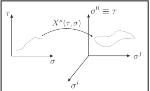
This is a (p = 1)-brane action, describing
Figure 2: Embedding of a string into a background spacetime. Note here that the coordinates, Xµ(τ, σ), are periodic in some directions. Thus giving a closed string.
a string propagating through a D dimensional spacetime. We will parameterize the worldsheet of the string, which is the two dimensional exten-sion of the worldline for a particle, by the two co-ordinates σ0 ≡τ and σ1 ≡ σ, with τ being
time-like andσ being space-like. The embedding of the string into the D dimensional background space-time is given by the functions (or fields)Xµ(τ, σ),
see figure 2.
Note that if we assumeσis periodic, then the embedding gives a closed string in the spacetime. Also, one should realize that the fields Xµ(τ, σ), which are parameterized by the worldsheet
coor-dinates, tell how the string propagates and oscillates through the background spacetime, and this propagation defines the worldsheet just as before with the fieldsXµ(τ),
param-eterized by the worldline coordinateτ, that described the propagation of the particle through spacetime where the propagation defined the worldline of the particle.
‡Note that if Tp has units of mass/vol, then the actionSp is dimensionless, as it should be, since
the measuredµp has units vol·length.
†Here Gαβ is the metric on thep+ 1 dimensional surface which is mapped out by thep-brane as
it moves through spacetime, whilegµν is the metric on theD dimensional background spacetime. For example, in the case of a string,p= 1,Gαβ is the metric on the worldsheet. Note that for the point particle the induced worldline metric is given by (since the worldline is one dimensional there is only one component for the induced metric)
∂Xµ∂Xν
Now, if we assume that our background spacetime is Minkowski, then we have that G00 = ∂X µ ∂τ ∂Xν ∂τ ηµν ≡X˙ 2, G11 = ∂X µ ∂σ ∂Xν ∂σ ηµν ≡ X 02 , G10 =G01= ∂X µ ∂τ ∂Xν ∂σ ηµν,
and thus, we have that
Gαβ = ˙ X2 X˙ ·X0 ˙ X·X0 X02 . (2.26)
From the form of the induced metric (2.26) we see that, in a Minkowski background,
det(Gαβ) = ( ˙X2)(X
02
)−( ˙X·X0)2. (2.27)
So our previous action reduces to
SN G =−T Z dτ dσ q ( ˙X·X0)2−( ˙X2)(X02 ), (2.28)
which is known as the Nambu-Goto action. This action can be interpreted as giving the area of the worldsheet mapped out by the string in spacetime. Since the equations of motion follow from minimizing the above action, one can think of the equations of motion for the string as the worldsheet of smallest area mapped out by the string in spacetime.
Now, in order to get rid of the square root, we can introduce an auxiliary field
hαβ(τ, σ) (this really is another metric living on the worldsheet, which is different from the induced metric Gαβ)‡, just like before with the auxiliary field e(τ). The resulting
action is called the string sigma-model, or Polyakov action, and it is given by
Sσ =−T 2 Z dτ dσ√−h hαβ∂X µ ∂α ∂Xν ∂β gµν, (2.29)
where h ≡ det(hαβ). Note that the above expression holds for a general background spacetime since we have not reducedGαβ for a Minkowski spacetime. Also note that at the classical level, the Polyakov action is equivalent to the Nambu-Goto action, while being better suited for quantization.
Proposition 2.2 The Polyakov actionSσ is equivalent to the Nambu-Goto actionSN G.
‡So, the worldsheet has an induced metric,Gαβ, from being embedded into the background
Proof First, note that varying any action with respect to a metric yields the stress energy tensorTαβ, i.e.
Tαβ =−2 T 1 √ −h δSσ δhαβ . (2.30)
Now, the equations of motion for the field hαβ follow from setting the variation in the
actionSσ with respect tohαβ equal to zero, δSσ = 0. When we varySσ w.r.t. hαβ and
set it equal to zero we have that
δSσ ≡ Z δSσ δhαβδh αβ = −T 2 Z dτ dσ√−h δhαβTαβ | {z } follows from (2.30) = 0,
which holds if and only ifTαβ = 0. So, computing Tαβ and setting the result equal to zero will give the equations of motion for the fieldhαβ.
Now to compute Tαβ we need to know what δhis. The claim is that
δh≡δ det(hαβ) =−hhαβδhαβ, (2.31) and to see this note that h = det(hαβ) = n!1α1···αnβ1···βnhα1β1 · · ·hαnβn. So, we have
that δh= 1 n! α1···αnβ1···βnh α1β1 · · ·hαnβn+ 1 (n−1)! α1···αnβ1···βnh α2β2 · · ·hαnβn =h α1β1h,
which implies that
δh=hαβδhαβh,
and also that
δh=−hαβδhαβh.
Putting these two together gives us,
δhαβh
αβ +hαβδhαβ = 0, (2.32)
which shows the previous claim, i.e. thatδh≡δ det(hαβ)
=−hhαβδhαβ.
Now, this gives us that
δ√−h=−1 2
√
−hδhαβhαβ, (2.33)
and so when we vary the Polyakov action we get
δSσ =−T
Z
dτ dσ√−h δhαβ− 1 2hαβh
which gives for the field equations ofhαβ, Tαβ ≡ −1 2hαβh γδ∂ γX·∂δX+∂αX·∂βX = 0. (2.35)
Thus, we have that
1 2hαβh γδ∂γX ·∂δX =∂αX·∂βX | {z } Gαβ , (2.36)
and taking the square root of minus the determinant of both sides gives that 1 2 √ −h hγδ∂ γX·∂δX = q −det(Gαβ), (2.37)
which shows thatSσ is equivalent, classically, to SN G. Q.E.D.
In the next chapter we will look at symmetries, both global and local, that our bosonic string theory possesses along with the field equations for the fieldXµ(τ, σ) and
the solutions to these field equations for different boundary conditions, open and closed strings.
2.4 Exercises Problem 1
Consider a point particle of massm and chargee moving in a flat background space-time under the influence of an electromagnetic field Aµ(X). If Xµ(τ) is the worldline
of the particle, then the dynamics of the point particle in this system can be described by the action: S =−1 4 Z d4XFµνFµν −mZ p−X˙2dτ +e Z AµX˙µdτ, (2.38) whereFµν =∂µAν −∂νAµ and ˙X2 =ηµνX˙µX˙ν, withηµν the flat Minkowski metric.
a) Find the equation of motion for Xµ(τ).
b) Show that the action (2.38) is invariant under gauge transformations of the electromagnetic field:
Aµ(X)→Aµ(X) +∂µΛ(X), (2.39)
where Λ(X) is any scalar function which vanishes at infinity. Problem 2
A relativistic quantum theory that includes gravity, involves three fundamental con-stants: the speed of light c, Planck’s constant ~ and Newton’s gravitational constant
G.
a) Determine the mass [M], length [L] and time [T] dimensions of each of these constants using dimensional analysis (namely, using physical relations which involve these quantities, such as Newton’s law of gravity).
b) Construct the combination of these constants which has dimension [L], and find its numerical value. This is called thePlanck length and is roughly the length scale at which we expect the effects of quantum gravity to become important.
c) Find the combination which has dimensions of mass, and thus compute the
Planck mass. Problem 3
Consider the action for a point particle:
S=−m
Z q
−gµν(X) ˙XµX˙ν dτ. (2.40)
As we saw in this chapter it can be equivalently written as:
˜
S0 = 1 2
Z
where e(τ) is an auxiliary field and ˙X2 = g
µν(X) ˙XµX˙ν. The action ˜S is invariant
under reparametrizations:
τ →τ0 =f(τ), (2.42)
provided that we transform e(τ) appropriately. Show that it is possible to use this reparametrization invariance to choose a gauge in whiche(τ) = 1.
Problem 4
Show that the p-brane Polyakov action with the addition of a cosmological constant Λp, Sσ =−Tp 2 Z dpτ dσ√−h hαβ∂αX·∂βX+ Λp Z dpτ dσ√−h. (2.43)
is equivalent to the “Nambu–Goto action”
SN G =−Tp
Z
dpτ dσp−det∂αX·∂βX, (2.44)
by choosing the “cosmological constant” Λp appropriately. (Hint: Solve the equations
3. Symmetries and Field Equations of the Bosonic String
Last week we saw that the action which de-scribes a string propagating in aDdimensional space-time, with given metric gµν, is given by
Sσ =−T 2
Z
dτ dσ√−h hαβ∂αXµ∂βXνgµν. (3.1) One advantage of the action is that, usually, it makes it easier to see whether the theory is invariant under a certain transformation or not.
3.1 Global Symmetries of the Bosonic String Theory Worldsheet
A global transformation in some spacetime is a transformation whose parameter(s) do not depend on where in the spacetime the transformation is being performed, i.e the derivative of any parameter with respect to any of the spacetime coordinates vanishes. A local transformation in some spacetime does however, depend on where the transfor-mation is begin performed in the spacetime. Examples of global transfortransfor-mations are rotations about an axis by some parameter θ, translations, etc. Whereas an example of a local transformation would be a rotation where the parameterθ(Xµ) does depend
on where in spacetime the rotation is being performed. Also, one should note that invariance of a theory under global transformations leads to conserved currents and charges via Noether’s theorem, while invariance under local transformations (or gauge transformations) is a sign of absent degrees of freedom in your theory. We will first discuss global transformations, namely the Poincar´e transformations, and then, in the next section, we will look at local transformations.
If we take our background spacetime to be Minkowskian then our bosonic string theory‡, which lives in this space, should have the same symmetries as Minkowski space
and, in particular, our theory should be invariant under the Poincar´e group. Poincar´e Transformations
These are global transformations of the form,
δXµ(τ, σ) =aµνXν(τ, σ) +bµ, (3.2)
δhαβ(τ, σ) = 0, (3.3)
‡Note that here we are really saying that the string worldsheet should have the same symmetries as
the background spacetime, namely the worldsheet should have the same symmetries as a Minkowski space.
where fields Xµ(τ, σ) are defined on the worldsheet, as is hαβ(τ, σ) and the aµ
ν, with
both indices lowered, is antisymmetric, i.e. aµν = −aνµ. This is indeed a global symmetry in the eyes of the worldsheet since the transformations do not depend on the worldsheet coordinates,σ and τ. We will now show that the aµ
ν generate the Lorentz
transformations.
According to Einstein’s theory of relativity, the speed of light is the same in all inertial frames, i.e. all inertial observers measure the same value for the speed of light. Thus, if (t, Xi) is the spacetime position of a light ray in one inertial frame and (t0, X0i
) in another, then the relation between the two is given by
ηµνXµXν = −c2t2+XiXi
= −c2t02+X0iX 0i
= ηµνX0µX0ν.
The linear transformations, denoted by Λ, which preserve this relation are called Lorentz transformations
X0µ = ΛµνXν. (3.4)
Infinitesimally, we have that the above transformation is given by
Λµν =δνµ+aµν. (3.5)
Note that we still have not shown that theaµ
ν in (3.5) is equal to the aµν in (3.2), we
are simply choosing the notation here because we are about to show that they are the same. The infinitesimal form of the Lorentz transformation says that
X0µ=Xµ+aµνXν,
which implies that the variation ofXµ, under the Lorentz transformation, is given by
δXµ =aµνXν. (3.6)
Now, if we impose that under a Lorentz transformation the spacetime interval vanishes,
δ
L.T.(ηµνX
then we have that δ L.T.(ηµνX µXν) = 2η µν(δXµ)Xν (3.7) = 2ηµν(aµkXk)Xν = 2akνXkXν = 0.
The most general solution to this is to have aµν = −aνµ, and thus we have that the two aµ
ν are equivalent to each other as proposed. Also, note that the first line of the
above equation, (3.7), is obtained by noting that ηµν is symmetric in its indices, i.e. δ(ηµνXµXν) =ηµν(δXµ)Xν+ηµνXµ(δXν) = 2ηµν(δXµ)Xν,
with the last equality above coming from exchangingµandνand noting thatηµν =ηνµ. We will now discuss some examples of Poincar´e transformations, namely the rota-tions and boosts:
1. For the first example of a Lorentz transformation, we will discuss that of a rotation around the X3 axis by an angleθ. For a four dimensional spacetime, the rotation
acts on the remaining two spatial coordinates as (finite transformation)
X01 = cos(θ)X1+ sin(θ)X2,
X02 =−sin(θ)X1+ cos(θ)X2.
Thus, for an infinitesimalθwe have, using the small angle approximations cos(θ)7→ 1 and sinθ7→θ, the transformations
X01 = X1+θX2,
X02 = −θX1+X2.
The infinitesimal transformations give us that δX1 = θX2 and δX2 = −θX1,
which shows that a1
2 = θ and a21 = −θ, while all other aµν are equal to zero.
Now, to see that aµν =−aνµ for this particular Lorentz transformation consider,
a12 = η1λaλ2 =η10a02+η11a12+η12a22+η13a32 =η11a12 =θ
a21 = η2λaλ1 =η20a01+η21a11+η22a21+η23a31 =η22a21 =−θ ,
2. Now we will look at a boost in the X0 and X1 directions by ϕ. The finite
transformations are given by
X00 = cosh(ϕ)X0+ sinh(ϕ)X1,
X01 = sinh(ϕ)X0+ cosh(ϕ)X1,
and thus for an infinitesimal ϕ we have, using the small angle approximations cosh(ϕ)7→1 and sinh(ϕ)7→ϕ, the transformations
X00 = X0+ϕX1,
X01 = ϕX0+X1.
The infinitesimal transformations give us that δX0 = ϕX1 and δX1 = ϕX0,
which shows that a0
1 = ϕ and a10 = ϕ, while all other aµν are equal to zero.
Finally, to show that the aµ
ν is antisymmetric consider,
a01 =η0λaλ1 =η00a01+η01a11+η02a21+η03a31 =η00a01 =−ϕ
a10 =η1λaλ0 =η10a00+η11a10+η12a20+η13a30 =η11a10 =ϕ ,
and so aµν =−aνµ.
Now that we have seen some concrete examples of Poincar´e transformations, the next question to ask is whether our Polyakov action is invariant under them. This would then imply that our bosonic string theory is Poincar´e invariant since the p= 1 brane action is equivalent with the Polyakov action. To see that the Polyakov action is indeed invariant under Poincar´e transformations consider the following,
δSσ =−T
Z
dτ dσ√−h hαβ∂α(δXµ)∂βXνgµν,
where we have used the fact thathαβ is invariant under the transformation, i.e. δhαβ =
0, and symmetry of the metric in its indices. Plugging in for the transformation on the coordinates, δXµ=aµ
kXk+bµ, we get that δSσ =−T
Z
This can be further simplified by noting that aµk and bk are not spacetime dependent
and thus we can drop thebk term and pull theaµ
k out of the parenthesis to give δSσ =−T
Z
dτ dσ√−h hαβaµk∂αXk∂βXνgµν.
Now, we can use the metric gµν to lower the upper index on aµk, doing this we get
δSσ =−T Z dτ dσ√−h aνk | {z } antisym hαβ∂αXk∂βXν | {z } sym ,
which is the product of an antisymmetric part with a symmetric part, and thus equal to zero. So, we have that, under a Poincar´e transformation, the variation in the Polyakov action is zero, δSσ = 0, which tells us that this action is invariant under these trans-formations.
3.2 Local Symmetries of the Bosonic String Theory Worldsheet
The next topic to be discussed is that of local symmetries and transformations on the worldsheet, i.e. transformations whose parameters depend on the worldsheet coordi-nates. What local symmetries does our bosonic string theory actually have?
1. Reparametrization invariance (also known as diffeomorphisms): This is a local symmetry for the worldsheet. The Polyakov action is invariant under the changing of the parameterσtoσ0 =f(σ) since the fieldsXµ(τ, σ) transform as scalars while the auxiliary field hαβ(τ, σ) transforms as a 2-tensor,
Xµ(τ, σ) =X0µ(τ, σ0) and hαβ(τ, σ) = ∂f
γ ∂σα
∂fδ
∂σβh0γδ(τ, σ0), (3.8)
Thus, our bosonic string is invariant under reparametrizations. This, as was men-tioned earlier, tells us that we have redundancies in our theory, i.e. we actually have fewer degrees of freedom than we thought. Also, note that these symme-tries are called diffeomorphisms, i.e. the transformations and their inverses are infinitely differentiable.
2. Weyl Symmetry: Weyl transformations are transformations that change the scale of the metric,
hαβ(τ, σ)7→h0αβ(τ, σ) = e2φ(σ)hαβ(τ, σ), (3.9) while leaving the scalars, Xµ(τ, σ), alone or, equivalently, under a Weyl
transformation since the parameter φ(σ) depends on the worldsheet coordinates. To see whether our bosonic string theory is invariant under a Weyl transformation we first need to see how both the quantities √−h and √−h hαβ transform. The
transformation of √−h is given by √ −h0 = q−det(h0 αβ) = e2(2φ(σ))/2 q −det(hαβ) = e2φ(σ)√−h .
While expanding (3.9) in φ yields thath0αβ =e−2φhαβ = (1−2φ+· · ·)hαβ, thus
the variation (infinitesimally) of hαβ is given by δhαβ = −2φhαβ. And so, for √
−h hαβ we have that
√
−h0 h0αβ =√
−he2φ(σ)e−2φ(σ)hαβ =√−h hαβ.
Thus, under a Weyl transformation Sσ does not change, or is invariant, which implies that the variation of Sσ under a Weyl transformation vanishes. This says that our bosonic string theory is invariant under Weyl transformations. We will now show that since our theory is invariant under Weyl transformations this implies that the stress-energy tensor associated with this theory is traceless,
hαβTαβ = 0. So, to begin recall that the stress-energy tensor is given by
Tαβ ≡ − 2 T 1 √ h δSσ δhαβ, (3.10)
which implies that, under a generic transformation of the field hαβ, we can write
the variation of Sσ as δSσ ≡ Z δSσ δhαβδh αβ =−T 2 Z dτ dσ√−h δhαβTαβ.
Thus, if we now restrict to a Weyl transformation we see that variation of the action becomes δSσ = −T 2 Z dτ dσ√−h δhαβTαβ = −T 2 Z dτ dσ√−h (−2φ)hαβTαβ,
which must be equal to zero since there is no variation in Sσ under a Weyl
transformation. Now, since √−h and φ are arbitrary this means that
hαβTαβ = 0, (3.11)
or that, for a Weyl invariant classical theory, the corresponding stress-energy tensor must be traceless.
Since our theory has local, or gauge, symmetries, we know that the theory has a redundancy in its degrees of freedom,§ and we can use these symmetries to cope with
these redundancies, this is known as gauge fixing. For example, in electrodynamics one has a symmetry under the group of phase transformations, i.e the Lie groupU(1) whose parameters are spacetime dependent, eφ(X). Now, for example, one can fix the gauge
by requiring that ∂µAµ = 0, known as the Lorenz gauge†, where Aµ is the gauge field
associated with the U(1) gauge group. By doing this one is able to remove some‡ of
the redundant degrees of freedom along with simplifying the description of the theory, since in the Lorenz gauge the Maxwell equations reduce to
Aν =ejν,
where e is a constant. Now, lets see how we can fix a gauge in order to simplify our bosonic string theory. In particular, we will now show that if our theory is invariant under diffeomorphisms and Weyl transformations then we can fix a gauge so that our intrinsic metric, hαβ, becomes flat.
First, note that since the metric,
hαβ = h00 h01 h10 h11 , (3.12)
is symmetric it has only three independent components,h00(X),h11(X), andh10(X) = h01(X). Now, a diffeomorphism (or reparametrization) allows us to change two of the
§This is because the worldsheet coordinates have no physical meaning, just like the parameter of
the worldline in relativistic physics has no meaning.
†Even though Lorentz is typically credited with this gauge choice, it was actually Lorenz who first
proposed it.
‡The Lorenz gauge is incomplete in the sense that there remains a subspace of gauge transformations
which preserve the constraint. These remaining degrees of freedom correspond to gauge functions which satisfy the wave equation
ψ= 0,
and to obtain a fully fixed gauge, one must add boundary conditions along the light cone of the experimental region.
independent components by using two coordinate transformations, f1(X) and f2(X),
to set h10(X) = 0 = h01(X) and h00(X) = ±h11(X) (where the ± depends on the signature of the metric). Thus, from our theory being diffeomorphism invariant, we see that our two dimensional metrichαβ(X) is of the formh(X)ηαβ. Now, we can use a Weyl transformation to remove this function, i.e. we then have thathαβ(X) =ηαβ. And so we see that if our theory is invariant under diffeomorphisms and Weyl transformations (there combinations are called conformal transformations), then the two-dimensional intrinsic metric, hαβ(X), can be “gauged” into the two-dimensional flat metric,
hαβ(X) =ηαβ = −1 0 0 1 . (3.13)
However, one should note that since gauge symmetries are local symmetries this ability to transform the metrichαβ(X) into in a flat metric is only valid locally and one cannot, in general, extend to the flat hαβ(X) to the whole worldsheet. Only if the worldsheet
is free of topological obstructions, i.e. its Euler characteristic is zero, can the locally flat metrichαβ(X) be extended to a globally flat metric on the worldsheet¶.
In terms of the gauge fixed flat metric, the Polyakov action becomes
Sσ = T 2
Z
dτ dσ( ˙X)2−(X0)2, (3.14) where ˙X ≡ dXµ/dτ and X0 ≡ dXµ/dσ. Finally, note that these two gauges are not
the only ones for our theory, i.e. even after we fix the reparametrization gauge and Weyl gauge to construct the flat metric it is still invariant under other local symmetries known as conformal transformations. These transformations will be discussed later on in subsequent lectures.
3.3 Field Equations for the Polyakov Action
Let us now suppose that our worldsheet topology allows for the gauge fixed locally defined flat metric hαβ to be extended globally. The field equations for the fields Xµ(τ, σ) on the worldsheet come from setting the variation ofSσ with respect toXµ7→ Xµ+δXµ equal to zero. This leads to
δSσ = T 2
Z
dτ dσ2 ˙XδX˙ −2X0δX0,
¶By being able to extend the locally flat intrinsic metric to the whole worldsheet implies that
there exists a flat coordinate system that covers the whole worldsheet. This, in turn, implies that the worldsheet has a flat geometry which implies that the Ricci curvature scalar vanishes. Now, since, in two dimensions, the Euler characteristic of a manifold is proportional to the integral of the Ricci curvature over the manifold, we see that being able to extend the locally flat metric requires for the Euler characteristic of the worldsheet to vanish.
and to proceed we integrate both terms by parts to give T Z dτ dσh−∂τ2+∂σ2XµiδXµ+ T Z dσX˙µδXµ ∂τ − T Z dτ X0δXµ σ=π+T Z dτ X0δXµ σ=0 .
We set the variation ofXµ at the boundary of τ to be zero, i.e. δXµ
∂τ = 0, and are
left with the field equations forXµ(τ, σ) for the Polyakov action,
−∂τ2+∂σ2Xµ−T Z dτhX0δXµ σ=π +X 0δXµ σ=0 i . (3.15)
Theσboundary terms tell us what type of strings we have, either closed or open strings.
• Closed Strings: For closed strings we take σ to have a periodic boundary condi-tion,
Xµ(τ, σ+n) =Xµ(τ, σ), (3.16) which implies that the boundary terms appearing in the variation of Sσ vanish since if Xµ(τ, σ + n) = Xµ(τ, σ) then δX(τ, σ = 0) = δX(τ, σ +n) and so
subtracting them gives zero. Thus, we are left with the following field equations for the closed string
∂τ2 −∂σ2Xµ(τ, σ) = 0, (3.17) with the boundary conditions
Xµ(τ, σ+n) =Xµ(τ, σ). (3.18)
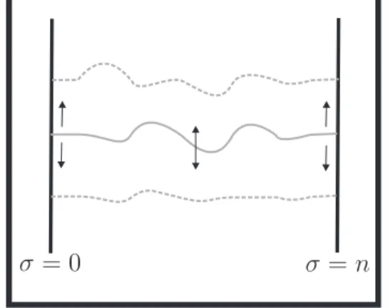
• Open Strings (Neumann Boundary Conditions): For the open string with Neu-mann boundary conditions we set the derivative of Xµ, by σ, at the σ boundary
to vanish, i.e. ∂σXµ(τ, σ+ 0) = ∂σXµ(τ, σ+n) = 0 (see figure 3). Under these
boundary conditions the boundary terms over σ also vanish and thus the field equations become
∂τ2 −∂σ2Xµ(τ, σ) = 0, (3.19) with the boundary conditions
Note that the Neumann boundary conditions preserve Poincar´e invariance since ∂σ(X0µ) σ=0,n = ∂σ(a µ νXν+bµ) σ=0,n = aµν∂σXν σ=0,n = 0.
• Open Strings (Dirichlet Boundary Conditions): For the Dirichlet boundary con-ditions we set the value ofXµto a constant at theσboundary,Xµ(τ, σ+0) =Xµ 0
and Xµ(τ, σ+n) =Xµ
n whereX µ
0 and Xnµ are constants (see figure 4). This also
makes the σ boundary terms vanish and so the field equations are
∂τ2 −∂σ2Xµ(τ, σ) = 0, (3.21)
with boundary conditions
Xµ(τ, σ= 0) =X0µ, (3.22)
and
Xµ(τ, σ=n) =Xnµ. (3.23)
Whereas the Neumann boundary conditions preserve Poincar´e invariance, the Dirichlet boundary conditions do not since
(X0µ) σ=0,n = (a µ νXν +bµ) σ=0,n =aµνX0,nν +bµ 6 =X0,nµ .
Thus, under a Poincar´e transformation the ends of the string actually change. Finally, note that if we have Neumann boundary conditions on p+ 1 of the back-ground spacetime coordinates and Dirichlet boundary conditions on the remaining
D−p+ 1 coordinates, then the place where the string ends is a Dp-brane.
So, we can see that under all three boundary conditions the resulting field equations are equivalent, just different boundary conditions. In addition to the above field equations,
Figure 3: Neumann BC’s: The string can oscillate and its endpoints can move along the boundaries as long as thier derivatives vanish at the bondaries.
Figure 4: Dirichlet BC’s: The string can osciallte but its endpoints are fixed at the boundary.
one must impose the field equations which result from setting the variation ofSσ with respect tohαβ equal to zero. These field equations are given by (see (2.35))
0 = Tαβ =∂αX·∂βX− 1 2hαβh
γδ∂γX·∂δX, (3.24)
and gauge fixing hαβ to be flat‡ we get that the field equations transform into the
following two conditions
0 =T00 =T11 = 1 2( ˙X
2+X02), (3.25)
and
0 = T01=T10 = ˙X·X0. (3.26)
3.4 Solving the Field Equations
Here again, we have and will assume that we can extend the gauge fixed flat metric to a global flat metric, hαβ 7→ ηαβ, on the worldsheet. Now, we will solve the system of equations by introducing light-cone coordinates for the worldsheet,
σ±= (τ ±σ), (3.27)
which implies that
τ = 1 2(σ
++σ−),
‡Recall that we have assumed that the topology on the worldsheet is such that we can extend the
local flat metric to a global flat metric and thus we can insert the flat metric into the field equations, which hold globally.
σ= 1 2(σ
+
−σ−).
The derivatives, in terms of light-cone coordinates, become
∂+ ≡ ∂ ∂σ+ = ∂τ ∂σ+ ∂ ∂τ + ∂σ ∂σ+ ∂ ∂σ = 1 2(∂τ +∂σ), ∂− ≡ ∂ ∂σ− = ∂τ ∂σ− ∂ ∂τ + ∂σ ∂σ− ∂ ∂σ = 1 2(∂τ −∂σ), and since the metric transforms as
ηα00β0 = ∂σγ ∂σα0 ∂σδ ∂σβ0ηγδ, we have that η++ =− ∂τ ∂σ+ 2 + ∂σ ∂σ+ 2 =−1 4+ 1 4 = 0, η−− =− ∂τ ∂σ− 2 + ∂σ ∂σ− 2 =−1 4+ 1 4 = 0, η+− =− ∂τ ∂σ+ ∂τ ∂σ− + ∂σ ∂σ+ ∂σ ∂σ− =− 1 4− 1 4 =− 1 2, η−+ =− ∂τ ∂σ− ∂τ ∂σ+ + ∂σ ∂σ− ∂σ ∂σ+ =− 1 4− 1 4 =− 1 2. Thus, in terms of light-cone coordinates, the metric is given by
ηαβ l-c c. =− 1 2 0 1 1 0 , (3.28) and so, ηαβ l-c c.=−2 0 1 1 0 . (3.29)
In terms of the light-cone coordinates, the field equations (∂2
τ −∂σ2)Xµ= 0 become
∂+∂−Xµ= 0, (3.30)
while the field equations for the intrinsic worldsheet metric,hαβ become
T++ =∂+Xµ∂+Xµ = 0, (3.31)