Learning an approximate model predictive controller with guarantees

Student Thesis204

Learning an Approximate Model Predictive Controller with

Guarantees

Student Thesis

Michael Hertneck

March

12

,

2018

Examiner:

Prof. Dr.-Ing. Frank Allgöwer

Supervisor:

Johannes Köhler, M.Sc.

Dr.sc. Sebastian Trimpe

Institute for Systems Theory and Automatic Control

University of Stuttgart

Prof. Dr.-Ing. Frank Allgöwer

Intelligent Control Systems Group

Abstract

In this thesis, a supervised learning framework to approximate a model predictive controller (MPC) with guarantees on stability and constraint satis-faction is proposed. The approximate controller has a reduced computational complexity in comparison to standard MPC which makes it possible to im-plement the resulting controller for systems with a high sampling rate on a cheap hardware. The framework can be used for a wide class of nonlinear systems.

In order to obtain closed-loop guarantees for the approximate MPC, a robust MPC (RMPC) with robustness to bounded input disturbances is used which guarantees stability and constraint satisfaction if the input is approximated with a bound on the approximation error.

The RMPC can be sampled offline and hence, any standard supervised learning technique can be used to approximate the MPC from samples. Neu-ral networks (NN) are discussed in this thesis as one suitable approximation method.

To guarantee a bound on the approximation error, statistical learning bounds are used. A method based on Hoeffding’s Inequality is proposed to validate that the approximate MPC satisfies these bounds with high confidence. This validation method is suited for any approximation method. The result is a closed-loop statistical guarantee on stability and constraint satisfaction for the approximated MPC.

Within this thesis, an algorithm to obtain automatically an approximate controller is proposed. The proposed learning-based MPC framework is illustrated on a nonlinear benchmark problem for which we learn a neural-network controller that guarantees stability and constraint satisfaction.

The combination of robust control and statistical validation can also be used for other learning based control methods to obtain guarantees on stability and constraint satisfaction.

Parts of this thesis have been submitted for publication at the IEEE Control Systems Letters. The title of the submitted paper is "Learning an Approx-imate Model Predictive Controller with Guarantees". The authors of the paper are Michael Hertneck, Johannes Köhler, Sebastian Trimpe and Frank Allgöwer.

Contents

2 Model Predictive Control - Theory 13 2.1 MPC problem formulation. . . 13 2.2 Robust MPC . . . 15 2.3 Approximate MPC . . . 17 3 Main approach 19 3.1 Problem formulation . . . 19 3.2 General approach . . . 20 4 Input robust MPC 21 4.1 RMPC formulation . . . 21 4.2 Constraint tightening . . . 22

4.3 Stability and constraint satisfaction. . . 25

4.3.1 Recursive feasibility . . . 25

4.3.2 Closed loop stability . . . 29

5 Approximation of the RMPC 35 5.1 Machine learning . . . 35

5.2 Neural networks . . . 36

5.2.1 Neural network basics . . . 36

5.2.2 Learning neural networks . . . 39

Contents

6 Automatic AMPC synthesis with guarantees 49

6.1 AMPC synthesis. . . 49

6.2 Automatic AMPC synthesis - step by step. . . 50

6.2.1 Step1: Show incremental stabilizability and Lipschitz constant . . . 50

6.2.2 Step2: Set accuracy . . . 54

6.2.3 Step3: Design of the RMPC . . . 54

6.2.4 Step4,5and6: Learning and validation . . . 57

7 Numerical example 59 7.1 System modeling . . . 59

7.2 Computation of the AMPC using Algorithm1 . . . 60

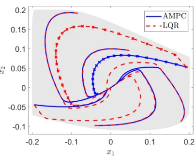
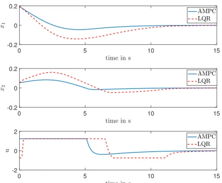
7.3 Simulation results . . . 63

7.3.1 Comparison to LQR . . . 64

7.3.2 Online computational demand . . . 65

8 Conclusion 67 8.1 Summary. . . 67

8.2 Future work . . . 68

Appendix 71 A.1 Numerical values for the verification of the local incremental stabilizability assumption . . . 71

1 Introduction

1.1 Problem description

Model predictive control (MPC) [1] is a modern control method which has been actively researched in the last years. It is based on repeatedly solving an optimization problem online. Applications in industry are widespread. An advantage of MPC is the guaranteed satisfaction of hard constraints and the optimality of the solution with respect to a certain cost function for nonlinear systems. One major drawback of MPC is the computational effort that arises when solving optimization problems online under real time requirements. This happens especially for settings with a large number of optimization variables, e.g if the prediction horizon is large, or if a high sampling rate is required.

For linear systems, the optimization problem can be solved offline i.e. before the runtime of the system under some mild assumptions [2]. Thus an explicit control law is obtained. The extension of [2] to nonlinear systems is not straightforward. Hence, the goal of this thesis is to develop a frame-work for approximating a nonlinear MPC through supervised learning with statistical guarantees on stability and constraint satisfaction.

1.2 Proposed approach

In this thesis, we propose a framework to learn a controller withguaranteed stability and constraint satisfaction. The key idea is to approximate a robust MPC (RMPC) with robustness to bounded input disturbances with a ma-chine learning technique. Any3regression method is admissible within the proposed framework, if the method is capable to satisfy the chosen bound on the approximation error. There are several machine learning techniques that can achieve an arbitrary small approximation error. In this thesis, we focus on neural networks which can approximate any nonlinear function with a finite number of nonlinearities arbitrary well [3]. However, in general, guaranteeing a bound on the approximation error for machine learning techniques can be challenging.

1 Introduction Robust MPC u = πMPC(x) +d Guarantees ifkdk_∞ ≤η Machine Learning Sample robust MPC Learn: πapprox ≈πMPC Validation Hoeffding’s Inequallity: P πapprox−πMPC _∞≤η≈1 Approximate MPC Statistical guarantees Constraint satisfac-tion and stability

Theorem7and

Theorem14

Lemma20

Theorem23

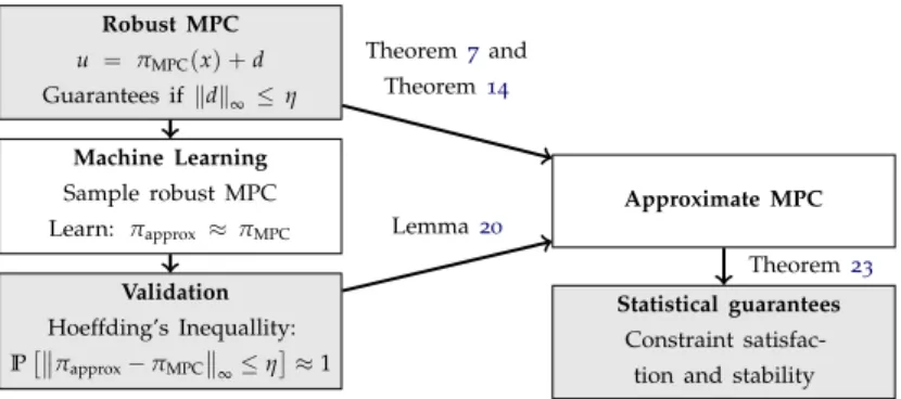
Figure1.1:Diagram of the proposed framework. We design an MPCπMPC

with robustness to input disturbances d. The resulting feedback law is sampled offline and approximated (πapprox) via machine learning techniques.

Hoeffding’s Inequality is used for validation to provide a bound on the error between approximate controller and MPC in order to guarantee stability and constraint satisfaction. The result is a controller with statistical guarantees.

A probabilistic approach to provide a bound on the approximation error is to use Hoeffding’s Inequality [4]. The resulting validation method is based on sampling the approximated RMPC and evaluate weather the approximation error satisfies a chosen bound. This probabilistic validation in combination with a learning method that is suitable to achieve any bound on the approximation error enables us to guarantee stability and the satisfaction of hard constraints with any desired probability. Therewith, a new method to obtain an approximate MPC can be established. A sketch of a complete framework for the controller synthesis based on the proposed methods is given in Figure1.1.

Advantages are the guarantees on stability and constraint satisfaction and a cheap implementable controller. The framework is suited to design controller for a wide class of nonlinear systems in an automatic fashion.

Instead of MPC and NN, other learning based control approaches as e.g. [5,6,7] can be adapted similar to the proposed framework, if a robust control method is used in combination with the proposed validation method. Thus, the proposed framework is also relevant for other learning based control methods.

1.3 Contribution

1.3 Contribution

This thesis makes contributions to the theory of learning based control and approximate MPC (AMPC). The main purpose is to propose a framework for the synthesis of an AMPC with guarantees on stability and satisfaction of hard constraints. The framework is applicable to a wide class of nonlinear systems. The controller synthesis using this framework works automated with few design parameters to choose.

One contribution of this thesis is to adjust results from tube based RMPC with guaranteed stability and constraint satisfaction for nonlinear systems [8] into a terminal cost/ terminal constraint setting with additive input distur-bance. The resulting RMPC guarantees stability and satisfaction of hard constraints under disturbance.

Another contribution of this thesis is a validation method that delivers guarantees on the approximation error in a probabilistic fashion based on Hoeffding’s Inequality [4]. Therefore, the learned control law is compared to the RMPC along trajectories. The key idea is, that stability and constraint satisfaction can be guaranteed for the closed loop system, if the approxima-tion error of the learned control law is smaller than the admissible input disturbance for the robust MPC. The bound on the approximation error is guaranteed probabilistic due to the validation method.

The combination of this contributions delivers a framework for the auto-matic controller synthesis to obtain an approximate MPC with guarantees on stability and constraint satisfaction.

The last contribution of this thesis is the application of the proposed framework to a continuous stirred tank reactor from [9] as benchmark. We show the practicability of the framework and substantiate that this method can yield a controller which guarantees closed loop stability and constraint satisfaction with a low computational complexity.

Parts of this thesis have been submitted for publication at the IEEE Control Systems Letters. The title of the submitted paper is "Learning an Approx-imate Model Predictive Controller with Guarantees". The authors of the paper are Michael Hertneck, Johannes Köhler, Sebastian Trimpe and Frank Allgöwer.

1 Introduction

1.4 Literature review

For linear systems, the optimization problem can be solved offline i.e. before the runtime of the system under some mild assumptions [2]. Thus an explicit control law is obtained. The extension of [2] to nonlinear systems is not straight forward and there are also computational complexity issues concerning the method from [2].

Hence, there exist several approaches to obtain an approximative solution for the MPC optimization. For linear systems, in [10] a learning algorithm is presented with additional constraints to guarantee stability and constraint satisfaction of the approximate MPC. This stands in contrast to our method, which uses standard learning methods and is applicable to nonlinear sys-tems.

For nonlinear systems, there are several approaches. One approach to ap-proximate MPC is convex multi parametric nonlinear programming [11,12], where a suboptimal approximation of the MPC control law is computed. Another approach is to approximate an MPC with machine learning tech-niques. This is done by neural networks in [13,14,15]. These methods can in general not provide guarantees on stability or constraint satisfaction for the approximated MPC which is especially crucial if hard state constraints are considered.

In [5], a support vector machine informed method is used to approximate the MPC. Stability and constraint satisfaction can be guaranteed for arbitrary small approximation errors based on inherent robustness properties. In [16], an MPC with Lipschitz based constraint tightening is approximated, which ensures stability for non vanishing approximation errors. The approximation error deduced in [5,16] is typically not achievable for practical application (compare example in Chapter 7) and is thus not suited for the proposed

framework.

1.5 Outline

This thesis is structured as follows: In Chapter2, we recap results from

the theory of MPC. In Chapter3, we formulate the problem and present

our main ideas. The input robust MPC is presented in Chapter4. In

Chapter5, we discuss supervised learning and present a validation method

to obtain guarantees on the learned MPC. In Chapter 6, the proposed

1.6 Notation

MPC offline is given. Chapter7contains a numerical benchmark example

for the framework. Chapter8concludes the thesis.

1.6 Notation

In this thesis, the following notation is used: The positive real numbers are denote byR>0, :={r∈R|r>0}, and respectively, R≥0 = R>0∪ {0}. A

function f is positive definite if f(0) =0 and f(x)>0∀x∈R∪ {0}. The functionsign(x)is defined as

sign(x) =    1 i f x>0 −1 i f x<0 0 else    . Class

K

A continuous functionα:R≥0→R≥0 is a classKfunction if it is strictly

increasing andα(0) =0. Sets and set operations

A setS is a robust positive invariant (RPI) set under some dynamics x(t+1) = f(x(t),w(t)), if x(t+1) ∈ S ∀x(t) ∈ S,∀w(t) ∈ W. The Minkovski set addition is defined asX⊕Y:={x+y:x∈X,y∈Y}. The Pontryagin set difference is defined byXY:={z∈Rn_{:z+y∈X,∀y∈Y}.}

Norms

The quadratic normkxk2=x>xis denoted byk·k. The quadratic norm with respect to a positive definite matrixQ=Q>is denoted bykxk2_Q=x>Qx. Eigenvalues

The minimum and maximum eigenvalue of a symmetric matrixQ=Q> are indicated byλmin(Q)andλmax(Q).λmax(P/Q)andλmin(P/Q)denote

the largest and smallest generalized eigenvalue of(P−λQ)v=0. P>0 implies thatλmin(P)>0 andP>Qdenotes thatλmin(P−Q)>0.

1 Introduction

Probabilistic expressions

2 Model Predictive Control - Theory

This chapter gives a brief overview over relevant MPC theory. First we recap some standard MPC methods to ensure stability and constraint satisfaction. Then, RMPC and AMPC are reviewed. A more detailed overview over well established results in MPC theory can be found in [1].

The basic idea of MPC is to use a dynamic model of a system to forecast the system behavior. Therewith an optimal input sequence can be computed and the first input of this sequence is used as feedback. Thus, contrary to most other control techniques, the control law is only implicit defined as the solution to an optimization problem. Satisfaction of constraints can be ensured by a suitable formulation of the optimization problem. An advantage of MPC is that complex nonlinear dynamics can be handled. We present a formulation for the MPC optimization problem that guarantees stability and constraint satisfaction in the next section.

2.1 MPC problem formulation

We consider the nonlinear discrete time dynamicsx(t+1) = f(x(t),u(t))

with continuous f, satisfying f(0,0) =0, wherex∈Rn_{denotes the system}

state andu∈Rm_{are the system inputs. The MPC optimization problem}

for setpoint stabilization for discrete time systems, the setpoint(x,u) = (0,0)

and a positive definite stage costl(x,u)can be stated as follows: For each time step, solve

VN(x) =min u(·|t)JN(x(t),u(·|t)) =min u(·|t) N−1

∑

2 Model Predictive Control - Theory subject to constraints x(t|t) =x(t), x(k+t+1|t) = f(x(k+t|t),u(k+t|t)), x(k+t|t)∈ X,k=0,...,N−1, u(k+t|t)∈ U,k=0,...,N−1, x(t+N|t)∈ X_f,

and applyu(t) =u?_{(t|t). The state and input constraints are denoted by}

Rn _{⊇ X ⊇0 andR}m _{⊇ U ⊇0,V}

f(x)the terminal cost and JN the open

loop cost. The prediction forx(k+t)at timetis denoted byx(k+t|t). The solutions of the MPC optimization problem is denoted withu?(·|t),x?(·|t)

and the value functionVN(x(t)). For continuous time systems, a similar

formulation is possible, for details see [1].

We call the MPC problem feasible at timet, if there exists at least one input ˜u(·|t)that satisfies the constraints . The MPC problem is recursive feasible if feasibility at timetimplies feasibility for all timesk+t,k∈N. We assume in the following chapters that the state can be measured. If the state can only be estimated, robust output feedback MPC is required, compare e.g. [17].

Stability results for MPC

The goals of model predictive control are to achieve stability of the origin x=0 for the resulting closed loop system and guaranteed satisfaction of state and input constraints for all times. Therefore, recursive feasibility of the optimization problem and closed loop stability have to be established using the finite horizon MPC optimization problem. Suitably designed terminal constraints and terminal costs for the MPC problem can be used to obtain this guarantees [18]. We sketch this procedure in this section.

To guarantee stability and constraint satisfaction, we use a suitable termi-nal costVf and a suitable terminal setXf [18]. Within the terminal set, an explicit control lawkf(x)∈ U ∀x∈ Xf ⊆ X, with

f(x,kf(x))∈ Xf ∀x∈ Xf,

needs to exist. Furthermore,

2.2 Robust MPC

must hold∀x∈ X_f. Then recursive feasibility of the MPC problem can be proven by considering the candidate solution

u(k+t|t+1) =

(

u(k+t|t) k=1,...,N−1 kf(x(N)|t+1) k=N

,

which guarantees that a solution that satisfies all constraints will exist at t+1 if it exists attdue to the terminal constraints. To show stability of the MPC, the value functionVN(x)can be used as Lyapunov function.

In [18], a procedure to compute terminal costs, a terminal set and a ter-minal controller for continuous time systems with stabilizable linearization at the origin and quadratic stage costs is provided. The method is termed Quasi Infinite Horizon MPC [18] as the cost functionJ_Nis an approximation of the infinite horizon cost.

On possibility to satisfies the assumptions on the terminal ingredients is a zero terminal constraint withVf(x) =0,Xf ={0}andkf(x) =0. However,

under disturbance, the satisfaction of this zero terminal constraint cannot be robustified using standard approaches.. Thus, for robust MPC, a zero terminal constraint is not suitable.

Further MPC schemes

There exist a lot of further MPC schemes with guarantees. In MPC without terminal constraints, stability of the closed loop system can be shown by choosing the prediction horizon large enough under some controllability assumptions [19,20]. This can bring computational benefits in comparison to MPC with terminal constraints but a longer prediction horizon may be necessary and the required controllability condition can be hard to verify. MPC without terminal constraints is equally applicable to our setup.

In economic MPC [21], the stage cost for the MPC optimization problem is not requested to be positive definite. As a result, the closed-loop system might not converge to an equilibrium, if other trajectories (e.g. periodic) exist, that lead to a better performance. The proposed framework is with modifications in the RMPC also applicable to economic MPC.

2.2 Robust MPC

In this section we review existing RMPC techniques. One of this methods will be extended in Chapter4to be robust with respect to input disturbances.

2 Model Predictive Control - Theory

This will enable us to approximate the RMPC algorithm with a machine learning tool to obtain an explicit MPC control law.

RMPC has to guarantee stability and constraint satisfaction for an uncertain (nonlinear) system for all possible realizations of the uncertainty. This is typically achieved by a constraint tightening. Assume an additive, bounded disturbance. Then, the disturbed system can be formulated as

x(t+1) = f(x(t),u(t)) +w(t)

withw(t)∈ W:{w(t)∈Rn_{| kw(t)k}

∞≤wmax,}.

Under some assumptions, inherent robustness properties of standard MPC formulations can be provided [22]. For inherent robustness, only arbitrary small disturbances may be admissible.

In Min-Max schemes the optimization problem is extended to find a control input that minimizes the predicted cost for the worst case disturbance, i.e. the disturbance that maximizes the cost. An overview over this approach is given in [23]. A disadvantage of Min-Max schemes is that the optimization may be computational intractable.

A compromise between inherent robustness and Min-Max schemes are tube based approaches. For linear systems, there are two main tube based approaches. In [24] an additional error feedback is used to keep the real system state in a tube around the nominal system state for the system dy-namics without disturbance. The tube is an RPI set for the system with error feedback under disturbance. The optimal nominal state for a given real sys-tem state is used as an additional optimization variable in the optimization problem. To achieve recursive feasibility, the state constraints are tightened by the size of the tube. The input constraints must be tightened according to the error feedback.

In [25], a constraint tightening with growing tubes is used for linear systems. If the system is stabilizable, a stabilizing controller can be used to obtain a bounded representation of the reachable system states after each time step along the prediction horizon if a disturbance occurs at the actual time step. The constraints are tightened such that the untightened constraints are still satisfied if one of this reachable system states occur. Since the pre-stabilized system is stable, the necessary constraint tightening is bounded for a bounded disturbance.

For nonlinear systems, there exist several tube based approaches. In Lipschitz based methods (e.g. [26]), a tightening of the state constraints based on a Lipschitz constant of the system is used. For unstable nonlinear

2.3 Approximate MPC

system dynamics, this approach leads to a constraint tightening which grows exponentially with the prediction horizon. Hence, the constraint tightening may be quite restrictive since the set of admissible states can decrease fast with growing prediction horizon. This can decrease the initial feasible region and the possible prediction horizon even for small disturbances. Even for small disturbances and a small prediction horizon, the tightened constraint set may be empty.

In [27], a RMPC with constraint tightening founded on an incremental input to state stability (δISS) using aδISS-Lyapunov function for uncertain systems is proposed. Based on the concept of local incremental stabilizability, [8] uses a constraint tightening similar, to the growing tubes approach for linear systems. With this approach a system with an additive state disturbance can be robustly stabilized. The constraint tightening grows along the prediction horizon but is bounded by a maximum value. This value depends on the maximum admissible disturbance. For small enough disturbances, this leads to a non empty constraint set for arbitrary large prediction horizons.

It may be perhaps premature to select a particular approach at the current stage of research [1]. Nevertheless, we present in Chapter4an adaption of

[8] to bounded input disturbances and terminal constraints and costs since this method allows a good trade off between computational complexity and limited conservatism.

2.3 Approximate MPC

One major drawback of MPC is the required computational effort for the online solution of the MPC optimization problem. Especially for settings with a large number of optimization variables, e.g. if the prediction horizon is large, or if a high sampling rate is required, the online optimization can get intractable for a lot of applications.

The goal of approximate MPC is to decrease the online computational effort by approximating the solution to the MPC optimization problem offline. This subsection deals with the problem of solving the optimization for the MPC algorithm offline to obtain an approximate control law. We require, that the control law can be written as a function of the states and does not need any iteration to solve it. Clearly, fast online evaluation of the approximate MPC control law must be possible.

2 Model Predictive Control - Theory

can be solved offline according to [2]. Therein, the MPC optimization is formulated as a multi parametric quadratic program. This can be used with the Karush-Kuhn-Tucker (KKT) conditions to obtain an explicit piece wise affine control law that guarantees the satisfaction of hard constraints.

Since the extension of [2] to nonlinear systems is not straight forward and since there are also complexity issues concerning the method from [2], there exist several approximate MPC approaches. For linear systems, [10] proposed to add constraints to the learning problem to ensure stabil-ity and constraint satisfaction of the suboptimal learned control law. An ansatz to approximate nonlinear MPC is convex multi parametric nonlinear programming [11,12], where a suboptimal approximation of the MPC is computed. The approximation of an MPC by neural networks, as also done herein, has for example been proposed in [14,15]. These methods can in general not provide guarantees on stability or constraint satisfaction with the approximated MPC. This is especially crucial if hard state constraints are considered.

In [5], a support vector machine informed method is used to approximate an MPC. Stability and constraint satisfaction can be guaranteed for arbitrary small approximation errors based on inherent robustness properties. In [16], an MPC with Lipschitz based constraint tightening is approximated, which ensures stability for non vanishing approximation errors. This method has the same drawbacks as Lipschitz based RMPC since the constraint tightening is too conservative which makes it impractical for the application to most nonlinear systems (compare e.g. the example in Chapter7).

We will present a novel approximate MPC approach with guarantees on stability and constraint satisfaction based on approximation of a RMPC in combination with a validation method based on Hoeffding’s Inequality in Chapter6.

3 Main approach

In this chapter, we pose the control problem and present the proposed approach.

3.1 Problem formulation

In this section, we introduce the control problem. We consider the following nonlinear discrete time system

x(t+1) = f(x(t),u(t)), (3.1) with the statex(t)∈Rn_{, the control inputu(t)∈R}m_{, the time stept∈N,}

and continuous f, satisfying f(0,0) = 0. We consider compact polytopic constraints

X =

x∈Rn_|Hx≤1

p ,U=u∈Rm|Lu≤1p ,

and a quadratic stage cost

l(x,u) =kxk2_Q+kuk2_R, (3.2) with a positive definiteQand a positive semidefiniteR. The control objective is to ensure constraint satisfaction, i.e.

(x(t),u(t))∈(X × U)∀t≥0, stability of the resulting system, which means

lim

t→∞x(t)→ ZRPI

for suitable initial conditions and a RPI setZ_RPI, and to minimize some cost function

∞

∑

k=0

3 Main approach

The resulting controller should be implementable on cheap hardware for systems with high sampling rates.

Our goal is to develop a framework for automatic controller synthesis. The framework has to be such that all computations can be done numerically with few design parameters.

3.2 General approach

We propose a framework based on approximating an MPC. The guarantees for stability and constraint satisfaction from MPC must be preserved under the approximation. This is achieved by modifying the MPC to be robust to bounded input disturbances.

The controller synthesis with the proposed framework works as follows: We set up an RMPC. The RMPC scheme guarantees stability and constraint satisfaction foru(t) =πMPC(x(t)) +d(t)withkd(t)k_∞≤ηwith a chosen bound on the input errorηand the RMPC feedback lawπMPC. The RMPC

is sampled offline over the set of feasible statesX_feas. The RMPC feedback is approximated using supervised learning techniques based on these samples. In this thesis we use NN to approximate the RMPC, even though any other supervised learning technique can be used within the framework. The learning yields an AMPC

πapprox:Xfeas→ U |u=πapprox(x).

With this controller, the closed-loop system is given by

x(t+1) = f(x(t),πapprox(x(t))). (3.3)

Hence, the AMPC feedbackπapprox(x)guarantees stability and constraint

satisfaction if the approximation errorπMPC−πapprox

∞is bounded by the

disturbance boundη, because then guarantees from the RMPC are preserved under approximation. We use a validation method based on Hoeffding’s Inequality to guarantee a desired boundηon the approximation error. The overall framework will be summarized in Algorithm1.

4 Input robust MPC

In this chapter, we present a formulation of an RMPC algorithm which pre-serves its guarantees on stability and constraint satisfaction under additive input disturbances. Hence, guarantees on stability and constraint satisfaction will be preserved if the RMPC is approximated with any approximation technique as long as the approximation error is below the bound on the admissible input disturbance of the RMPC. The chapter is organized as follows:

An RMPC formulation with robustness to additive input disturbances based on a constraint tightening is introduced in Section4.1. The scheme

is an adaption of [8], where a robust MPC scheme for systems under state disturbances and without terminal constraints is presented. In Section4.2,

we present the constraint tightening method based on a growing tube along the prediction horizon for open loop trajectories in the RMPC optimization problem. The tube is subtracted from the constraint set. In the last section, recursive feasibility and closed loop stability for the perturbed system with bounded input disturbance are proven.

4.1 RMPC formulation

To achieve the robustness of the RMPC, we use a quasi infinite horizon MPC formulation [18] with robust constraint tightening [8], which can be formulated as VN(x(t)) =min u(·|t) JN((x(t)),u(·|t)) =min u(·|t) N−1

∑

4 Input robust MPC subject to constraints x(t|t) =x(t), (4.1b) x(k+t+1|t) = f(x(k+t|t),u(k+t|t)), (4.1c) x(k+t|t)∈ X¯_k,k=0,...,N−1, (4.1d) u(k+t|t)∈ U¯_k,k=0,...,N−1, (4.1e) x(N+t|t)∈ Xf. (4.1f) We denote the set of states where (4.1) is feasible byX_feas. The solution

of the RMPC optimization problem (4.1) is denoted byu?(·|t). The RMPC

feedback at timetisπMPC(x(t)):=u?(t|t). The state and input constraints

from standard MPC formulations are replaced by tightened constraints ¯X_k

and ¯U_k. The design of the terminal ingredientsX_f and Vf will be made

precise later. The closed loop of the RMPC under disturbance is given by x(t+1) = f(x(t),πMPC(x(t)) +d(t)), (4.2) with

d(t)∈ W={d∈Rm_:kdk

∞≤η},∀t≥0 (4.3) for someη. We present in the next subsection, how the constraint tightening for the RMPC is done for a chosen bound on the input disturbance.

4.2 Constraint tightening

In this section, we state the constraint tightening and necessary assump-tions for the RMPC to guarantee stability and constraint satisfaction under approximation. The constraint tightening is based on a local incremental stabilizability condition and depends on an exponential contraction rateρ. Hence, the following assumption is used in order to design the RMPC:

Assumption1. (Local incremental stabilizability [8,28]) There exists a control law κ:X × X × U →Rm, aδ-Lyapunov function V_δ:X × X × U →R≥0, that is

continuous in the first argument and satisfies V_δ(x,x,v) = 0∀x ∈ X, ∀v ∈ U, and parameters cδ,l, cδ,u δloc, kmax ∈ R>0,ρ ∈ (0,1), such that the fol-lowing properties hold for all(x,z,v) ∈ X × X × U,(z+,v+) ∈ X × U with Vδ(x,z,v)≤δloc:

c_δ,lkx−zk2≤V_δ(x,z,v)≤c_δ,ukx−zk2, (4.4)

kκ(x,z,v)−vk ≤kmaxkx−zk, (4.5) V_δ(x+,z+,v+)≤ρV_δ(x,z,v), (4.6)

4.2 Constraint tightening

with

x+= f(x,κ(x,z,v)),z+ =f(z,v).

Remark2. Assumption1is for example fulfilled, if the linearized dynamics at any point(x,v)∈ X × Uare stabilizable with a common quadratic Lyapunov function V=x>Px and f is locally Lipschitz. Hence, Assumption1is not very restrictive.

The concept of incremental stability [8] describes incremental robustness properties, and is thus suited for the analysis of perturbed trajectories in the RMPC design. Note that neitherVδnorκ need to be known explicitly to design the RMPC. Only the exponential decay rateρand boundsc_δ,l,cδ,u andkmaxare used within the RMPC design for the constraint tightening.

These parameters are computed for an example system in Chapter7.

To overestimate the influence from the system input on the system state, we use the following assumption:

Assumption3. (Local Lipschitz continuity of the input) There exists aλ∈ R, such that∀x∈ X,∀u∈ U,∀u+d∈ U

kf(x,u+d)−f(x,u)k ≤λkdk_∞. (4.7) With this assumption, we can introduce a bound on the admissible input disturbance which will be used in the proof of robust stability and recursive feasibility for the RMPC:

Assumption4. (Bound on the input disturbance) The input disturbance bound satisfies

η≤η1:= _λ1

q δloc

cδ,u.

Note that the polytopic setWcontains all admissible input disturbances. The set

Ut=U W

ensures thatu+d∈ U ∀u∈ Ut. SinceUandWare polytopic, we can write Utas Ut=u∈Rm|Ltu≤1p . We set ex:=ηλ s c_δ,u c_δ,l kHk_∞,eu=ηλ s c_δ,u c_δ,l kLtk_∞kmax. (4.8)

4 Input robust MPC

Therewith, the constraint tightening is achieved with scalar tightening pa-rameters ek,x:=ex 1−√ρk 1−√ρ,ek,u: =eu 1−√ρk 1−√ρ, k ∈ {0, ...,N},

based on the exponential contraction rate ρ, ex and eu. The tightened

constraint sets are given by ¯

X_k:= (1−ek,x)X ={x∈Rn|Hx≤(1−ek,x)1p},

¯

U_k:= (1−ek,u)Ut={u∈Rm|Ltu≤(1−ek,u)1q}.

Note that, ifkapproaches infinity, we get

X_∞:= (1−e_∞,x)X, U∞:= (1−e_∞,u)Ut,e_∞,x:= ex

1−√ρ,e∞,u:= eu

1−√ρ. Contrary to Lipschitz based tightening approaches as in [26], the constraint tightening is bounded even as k approaches infinity. Ifηis chosen small enough, the tightened constraint sets are not empty for allk.

Clearly, the size of the tightened constraints depends onexandeuand

thus onη. Hence, decreasing the approximation accuracyηincreases the feasible region.

The maximum influence of a disturbance at the current time step on the predicted system statex(N+t|t)is described by

WN= ( x∈Rn:kxk ≤λη s ρNcδ,u cδ,l ) . (4.9)

We use the following Assumption on the terminal set to guarantee recursive feasibility and closed loop stability similar to [18,29,30]

Assumption 5. (Terminal set) There exists a local control Lyapunov function Vf(x) =kxk2P, a terminal setXf =

n

x∈Rn_|V

f(x)≤αf

o

and a control law kf

such that∀x∈ X_f

f(x,kf(x)) +w∈ Xf,∀w∈ WN, (4.10) Vf(f(x,kf(x)))≤Vf(x)−l(x,kf(x)), (4.11)

4.3 Stability and constraint satisfaction

Remark6. For continuous time systems [18] provides the existence of a terminal set if the linearization of(3.1)is stabilizable and(0,0)lies in the interior ofX × U.

Furthermore an approach to calculate the terminal set is stated. In [30], the results from [18] are adapted to discrete time systems. These approaches are both for systems without disturbances. For a disturbed system, a terminal set can be calculated by using the approach from [30] forX¯_N×U¯_N instead ofX × U. Then, there will always be a small enoughηor a large enough N to ensure that(4.10)is satisfied.

This has resemblances to [29]. We show, how this can be done in Section6.2.3.

4.3 Stability and constraint satisfaction

In this section we study the properties of the RMPC closed loop system (4.2)

under disturbance. First, recursive feasibility of the RMPC under disturbance for an initial feasible point is proven in Theorem7. Then, Lemma11and

Propositions12and13deliver the prerequisites to prove the stability of the

closed loop system as it is done in Theorem14.

4.3.1 Recursive feasibility

First we show recursive feasibility of the MPC-algorithm with the following theorem:

Theorem 7. Let Assumptions 1, 3, 4 and5 hold. Assuming that there is a feasible input sequence u?_{(·|t)for problem(}4.1)at time t, a feasible input sequence

¯

u(·|t+1)for system(4.2)under input disturbance at time t+1can be constructed

as follows: ¯ u(k+t|t+1) = ( κ(x¯(k+t|t+1),x?(k+t|t),u?(k+t|t)), 1≤k≤N−1 κ(x¯(k+t|t+1),x?(k+t|t),kf(x?(k+t|t))), k=N , (4.13) The corresponding state sequence is given byx¯(k+t|t+1),k=1, . . . ,N with

¯ x(k+t+1|t+1) =f(x¯(k+t|t+1), ¯u(k+t|t+1)), k=1,...,N, ¯ x(t+1|t+1) =x(t+1) = f(x(t|t),u?(t|t) +d(t)),kd(t)k_∞≤η. =x?(t+1|t) +4x, k4xk ≤λη, .

4 Input robust MPC

Proof. The proof is composed of two parts. Part I shows the satisfaction of state constraints (4.1d) and input constraints (4.1e). Part II establishes the

satisfaction of the terminal constraint (4.1f).

Part I:Fork ≤ N, it holds thatx?_{(k+t|t) ∈} X¯_kdue to (4.1d) and (4.1f).

By (4.1e),u?(k+t|t) ∈U¯_k fork <N. Furthermore, defineu?(N+t|t) =

kf(x?(t+N|t))withkf(x?(t+N|t))∈U¯N by (4.12) and (4.1f) as input at

timet+N. By Assumption3and (3.3) it holds that

kx¯(t+1|t+1)−x?(t+1|t)k ≤λku(t)−u?(t|t)k_∞≤λη.

The boundη≤η1from Assumption4impliesV

δ(x(t+1),x?(t+1|t),u?(t+ 1|t))≤δloc. Using (4.6) recursively, we get

Vδ(x¯(k+t|t+1),x

?_(k+t|t),u?_(k+t|t))≤

ρk−1cδ,uλ2η2≤δloc. (4.14) With (4.4) and (4.5) this yields

kx¯(k+t|t+1)−x?(k+t|t)k ≤ s ρk−1cδ,u c_δ,lλη, (4.15) ku¯(k+t|t+1)−u?(k+t|t)k ≤ s ρk−1cδ,u c_δ,l kmaxλη. (4.16) Note thatk.k_∞≤ k.kand

Hx¯(k+t|t+1)−Hx?(k+t|t) =H(x¯(k+t|t+1)−x?(k+t|t)). With the choice ofex from (4.8) we can overestimate

Hx¯(k+t|t+1)≤Hx?(k+t|t) +kHk_∞ s ρk−1cδ,u c_δ,lλη1p (4_.8₎ ≤Hx?(k+t|t) +√ρk−1ex1p≤(1−ek,x+ √ ρk−1ex)1p = (1−ek−1,x)1p. (4.17) The same procedure for the input with

4.3 Stability and constraint satisfaction delivers Ltu¯(k+t|t+1)≤Ltu?(k+t|t) +kLtk_∞ q ρk−1c_δ,lkmaxλη1q (4_.8₎ ≤Ltu?(k+t|t+1) + √ ρk−1eu1q≤(1−ek,u+ √ ρk−1eu)1q = (1−ek−1,u)1q. (4.18) From (4.17) and (4.18) it follows that

¯

u(k+t|t+1)∈U¯_k−1, ¯x(k+t|t+1)∈X¯k−1, 1≤k≤N.

The choice ofUt, i.e.U0=Utguaranteesu?(t|t) +d(t)∈ U,∀d(t)∈ W.

Part II: recursive satisfaction of the terminal constraintsThe recursive satis-faction of the terminal constraints is guaranteed by the application of the terminal controller for ¯u(N+t|t+1). For the unperturbed system at time t+N+1 predicted at timetifkf is applied at timet+N, it holds that

x?(N+1+t|t) =f(x?(N+t|t),u?(N+t|t)), u?(N+t|t) =kf(x?(N+t|t)).

Due to (4.15) it holds that

¯

x(t+N+1|t+1) =x?(t+N+1|t) +w, w∈ WN.

Therefore with (4.10) andx?(t+N|t) ∈ X_f from (4.1f), the recursive

satisfaction of the terminal constraint can be shown with ¯

x(t+N+1|t+1) =x?(t+N+1|t) +w∈ X_f ∀w∈ W_N.

Remark8. Instead of choosing an approximation accuracyη, it is also possible to chose a maximum constraint tightening. This induces a bound onexandeu. Then, ηmust be chosen such that it satisfies the following inequalities:

η≤η1 (4.19) η≤η2:= s c_δ,l cδ,u ex λkHk_∞ ( 4.20) η≤η3:= s c_δ,l c_δ,u eu λkLtk_∞kmax . (4.21)

4 Input robust MPC

Corollary9. If (4.5)from Assumption1is modified to kκ(x,z,v)−vk ≤˜kmax

q

Vδ(x,z,v), then, the less conservative bound

eu=ηλ√cδ,uk˜maxkLtk_∞

can be used.

Proof. Replace (4.16) in the proof for Theorem7by ku¯(k+t|t+1)−u?(k+t|t)k =kκ(x¯(k+t|t+1),x?(k+t|t),u?(k+t|t))−u?(k+t|t)k ≤_k˜_maxq_V δ(x¯(k+t|t+1),x?(t+1|t),u?(t+1|t)) ≤_k˜_maxq_ρk−1_c δ,uλη.

Then the remainder of the proof for Theorem7can be used.

Corollary10. Suppose that Assumption1is satisfied with V_δ(x,z,v) =kx−zk2_Pr

andκ(x,z,v) = K(x−z) +v with Kr, Pr matrices parameterized by the point

r= (z,v). Assume further, that

kx−zk2_P

r≤1⇒ kH(x−z)k∞≤c1 (4.22)

and

kx−zk2_P

r≤1⇒ kLtKr(x−z)k∞≤c2. (4.23)

Then we can replaceexandeufrom(4.8)by the less conservative constraints

˜ ex:=ηλ√c_δ,uc1, ˜eu=ηλ√c_δ,uc2. Proof. (4.14) delivers V_δ(x,z,v) =kx−zk_P2_r≤ρk−1cδ,uλ 2 η2

which implies due to (4.22)

kH(x¯(k+t|t+1)−x?(k+t|t))k_∞≤

q

4.3 Stability and constraint satisfaction

Hence, (4.17) can be rewritten as

Hx¯(k+t|t+1)≤Hx?(k+t|t) +kH(x¯(k+t|t+1)−x?(k+t|t))k_∞1p ≤Hx?(k+t|t) + q ρk−1cδ,uλc1η1p ≤(1−e˜k,x+ √ ρk−1e˜x)1p= (1−e˜k−1,x)1p.

The proof for ¯u(k+t|t+1)can be done in the same way.

This may deliver a less conservative constraint tightening, but the verifica-tion of (4.22) and (4.23) may be more challenging than the computation of

the bounds in Assumption1.

4.3.2 Closed loop stability

Due to the input disturbance, asymptotic stability of a setpoint cannot be guaranteed. Instead, we show that an RPI setZ_RPIcan be stabilized. Since we do not assume control invariance of the constraint setX, convergence can only be established for all initial conditions in some region of attraction

X_feas. The shape of the setZ_RPI can be characterized with the following Lemma.

Lemma11. ([8] Lemma7) Let the value function VNsatisfy

kx(t)k2_Q≤VN(x(t))≤γkx(t)k2_Q (4.24) VN(x(t+1))−VN(x(t))≤ −kx(t)k2Q+w¯ (4.25)

for all x(t) ∈ X_ROA ={x|VN(x)≤Vmax}, with constantsγ, ¯w,Vmax∈ R>0.

For Vmax ≥γw¯ =: VRPI, the setZRPI :={x|VN(x)≤VRPI}is robustly

stabi-lized for all initial conditions x(0)∈ XROA.

In Proposition12a continuity like property of the value functionV_N(x)

will be established. This helps us to apply Lemma 11 in the proof of

convergence.

Proposition12. Let Assumptions1,3,4and5hold. Given a Vmax∈R>0. Then

the value function VNsatisfies for all x(t)∈ {x|VN(x)≤Vmax}

4 Input robust MPC

whereαη,Vmax is a classKfunction with

αη,Vmax(η) = 1−ρN 1−ρ cmaxλ 2 η2+2pVmaxcmax 1−√ρN 1−√ρ λη +2 q αfdmaxρNλη+dmaxρNλ2η2. (4.26)

with cmax:= (λmax(Q) +k2maxλmax(R))c_cδ,u

δ,l and dmax:=λmax(P)

cδ,u

cδ,l.

Proof. Consider the candidate solution (4.13). Since this is a feasible solution,

is holds that VN(x(t+1))≤JN((x¯(t+1)), ¯u(·|t+1)) = N

∑

The quadratic stage cost of the candidate solution (4.13) satisfies for

1<k<N l(x¯(k+t|t+1), ¯u(k+t|t+1)) =kx¯(k+t|t+1)k2_Q+ku¯(k+t|t+1)k2_R =kx?(k+t|t) + (x¯(k+t|t+1)−x?(k+t|t))k2_Q +ku?(k+t|t) + (u¯(k+t|t+1)−u?(k+t|t))k2_R ≤kx?(k+t|t)k2_Q+ku?(k+t|t)k2_R +kx¯(k+t|t+1)−x?(k+t|t)k2_Q +ku¯(k+t|t+1)−u?(k+t|t)k2_R +2kx?(k+t|t)k_Qkx¯(k+t|t+1)−x?(k+t|t)k_Q +2ku?(k+t|t)k_Rku¯(k+t|t+1)−u?(k+t|t)k_R. (4.27) From (4.15) and (4.16) we can derive

kx¯(k+t|t+1)−x?(k+t|t)k2_Q+ku¯(k+t|t+1)−u?(k+t|t)k2_R≤cmaxρk−1λ2η2 with cmax := (λmax(Q) +k2maxλmax(R))c_cδ,u

δ,l. Given a Vmax ∈ R>0 with

VN(x(t))≤Vmaxit follows that

4.3 Stability and constraint satisfaction

Hence, (4.27) implies

l(x¯(k+t|t+1), ¯u(k+t|t+1))≤l(x?(k+t|t),u?(k+t|t))

+cmaxρk−1λ2η2+2pVmaxcmax

√

ρk−1λη. (4.28)

Furthermore, withx?(N+1+t|t) = f(x?(N+t|t),kf(x?(N+t|t))the

ter-minal costs satisfy

Vf(x¯(t+N+1|t+1)) =kx¯(t+N+1|t+1)k2P =kx?(t+N+1|t) + (x¯(t+N+1|t+1)−x?(t+N+1|t))k2_P ≤kx?(t+N+1|t)k2_P+2kx?(t+N+1|t)k_Pkx¯(t+N+1|t+1)−x?(t+N+1|t)k_P +kx¯(t+N+1|t+1)−x?(t+N+1|t)k2_P ≤Vf(x?(t+N+1|t)) +2 q αfdmaxρNλη+dmaxρNλ2η2 (4.29)

withdmax:=λmax(P)c_cδ,u

δ,l andVf(x ?_{(t+N+1|t+1))≤} αf. Consider VN(x(t+1))−VN(x(t)) ≤ N

∑

∑

∑

cmaxρk−1λ2η2−2pVmaxcmax

√ ρk−1λη

−l(x?(t|t),u?(t|t))−Vf(x?(N+t|t)).

4 Input robust MPC

x?(t+N|t)∈ X_f this can be modified to VN(x(t+1))−VN(x(t)) (4.28),(4.29) ≤ l(x?(N+t|t),u?(N+t|t)) +Vf(x?(N+1+t|t+1)) −l(x?(t|t),u?(t|t))−Vf(x?(N+t|t)) + N

∑

cmaxρk−1λ2η2−2pVmaxcmax

√ ρk−1λη +2qαfdmaxρNλη+dmaxρNλη ≤Vf(x?(N+1+t|t+1)) +l(x?(N+t|t),kf(x?(N+t|t)) −Vf(x?(N+t|t))−l(x?(t|t),u?(t|t)) +αη,Vmax(η) (4_.11₎ ≤ −l(x?(t|t),u?(t|t)) +αη,Vmax(η). Note that l(x(t),u(t)) =kxk2_Q+kuk2_R≥ kxk2_Q. Therefore it holds that

VN(x(t+1))−VN(x(t))≤ −kxk2Q+αη,Vmax(η). (4.30)

Another prerequisite for the proof of stability of the closed loop system (3.3) is a bound onV_N(x)in terms ofkxk2

Q. This bound is established in the

following proposition:

Proposition 13. Let Assumption 5hold. Given Vmax ∈ R>0. Then for all

VN(x)≤Vmaxit holds that

kxk2_Q≤VN(x)≤γkxk2_Q withγ:=λmax(P/Q)max

n

Vmax

αf ,1

o . Proof. For allx∈ X_f, it holds that

4.3 Stability and constraint satisfaction

With

kxk2_Qλmax(P/Q)≥ kxk2P

and Assumption5, it follows for allx∈ X/ _f, kxk2_Q> αf

λmax(P/Q).

Together withVN(x)≤Vmax, this implies

VN(x)≤

Vmax

αf

λmax(P/Q)kxk2Q.

As a result, it holds that

VN(x)≤ kxk2Qλmax(P/Q)max ( Vmax αf ,1 ) | {z } :=γ . (4.31)

The lower bound follows direct from the definition ofVN(x).

Now we are ready to state the theorem which guarantees closed loop convergence toZ_RPI:

Theorem14. Let Assumptions1, 3, 4and5hold. Given Vmax ∈ R>0. Then

for the closed loop system(3.3)the setZ_RPI :={x|V_N(x)≤V_RPI}with V_RPI:= αη,Vmax(η)γ ≤ Vmax is stabilized for all initial conditions x(0) ∈ XROA

={x|VN(x)≤Vmax} ⊆ Xfeasand all disturbances d(t)∈ W.

Proof. By Proposition12, (4.30) holds for all initial conditionsx(0)∈ X_ROA= {x|VN(x)≤Vmax}. From the initial feasibility follows as proven in

Theo-rem 7 the recursive feasibility. Take _α

η,Vmax from Proposition 12 and γ

form Proposition13. SinceV_N(x(t+1))−V_N(x(t))≤ −kxk2

Q+αη,Vmax(η)

andkxk2_Q ≤ VN(x(t)) ≤ γkx(t)k2_Q, Lemma11can be used. Hence, the

setZRPI:={x|VN(x) =VRPI}withVRPI:=αη,Vmax(η)γis stabilized for all

initial conditionsx(0) ∈ X_ROA ={x|VN(x)≤Vmax}and all disturbances

d(t)∈ W.

Corollary15. The size ofZ_RPIfrom Theorem14depends on the input error bound η. Ifηis chosen small enough,ZRPI∈ Xf and asymptotic stability of the origin

can be guaranteed by applying the terminal controller once the system state enters the terminal set.

4 Input robust MPC

Proof. Due to (4.31) it holds that ZRPI⊆Z˜ := x∈Rn_{| kxk}2_≤ αη,Vmax(η)γ λmax(Q) . Furthermore, it holds that

X_f ⊇X˜_f := x∈Rn_{| kxk}2_≤ αf λmin(P) . The condition αη,Vmax(η)< λmax(Q)αf λmin(P)γ ( 4.32) implies Z_RPI⊆Z ⊆˜ X˜_f ⊆ X_f.

Sinceαη,Vmaxis a classKfunction inη,η>0 can be chosen such thatαη,Vmax

can get arbitrary small and hence (4.32) holds. Thus, if the disturbance is

small enough,ZRPI lies inXf and the system converges to the interior of X_f. InsideX_f, the terminal controller can be applied to achieve asymptotic stability.

5 Approximation of the RMPC

In this chapter, we state an approach to learn a control law using supervised learning in detail. First we recap useful results from machine learning theory to approximate the RMPC. Then, we introduce a probabilistic validation method for the resulting controller.

The chapter is structured as follows: In Section5.1we present machine

learning in general. In Section5.2, we recap important results from the

theory of NN and discuss how a NN can be used to learn the RMPC. Since it is challenging to verify a bound on the approximation error for a learned control law, in Section5.3we present a validation method based on

Hoeffding’s Inequality. With this validation method, it is possible to deliver a probabilistic bound on the approximation error of the learned control law and hence to deliver guarantees on stability and constraint satisfaction for the AMPC what will be the subject of the Chapter6.

5.1 Machine learning

This section covers the topic of machine learning in general. According to [31], machine learning can be described as the process of how a machine can learn specific tasks by an algorithm to obtain a general rule. This rule has to work on examples which were used to learn and has to be generalizable to previously unseen, new examples. According to [32] this is based on data and not on modeling the rule. [32] distinguishes between three types of learning. For supervised learning, learning data contains explicit example inputs and corresponding outputs for the desired task. Reinforcement learning is based on input data without the target output. Instead, it contains some possible output together with a measure how good that output is. Unsupervised learning does not depend on output information for the learning data. Therefore it is rather a clustering of inputs which may belong together. In the following, we focus on the supervised learning problem since we can compute a unique output for an arbitrary number of inputsx∈ X_feasfor the RMPC algorithm (4.1).

5 Approximation of the RMPC

The supervised learning problem

We define the supervised learning problem similar to [32] as follows:

Definition 16. (Supervised learning) There is an input x ∈ X_feas, an output u ∈ U and an unknown target functionπMPC : Xfeas → U where Xfeas is

the input space andU is the output space. There is a data set DofΠsamples of inputs and corresponding outputs(xi,ui) with ui = πMPC(xi), i = 1,...,Π.

Furthermore, there is a learning algorithm that uses the data setDto pick a function

πapprox:Xfeas→ Uthat approximatesπMPCfrom a hypothesis setH. The process

of choosingπapproxis called supervised learning.

Clearly, we can produce an arbitrary number of samples(x,πMPC(x))to

use them for the learning step.

According to [31], we distinguish further between regression and classifi-cation. For classification problems, the output space contains a finite number of elements, the classes. Regression problems have an output space with infinite many elements. The problem of learning an MPC is a regression problem since the desired outputπMPCis continuous valued. We focus in

this thesis on NN which can be used for both, regression and classification. Other function approximator that can learn essentially any nonlinear function arbitrary well are for example Gaussian processes [33] and support vector machines [34]. They could be used in our AMPC framework as well instead of NN.

5.2 Neural networks

In this section we recap NN for regression according to [35,36]. NN can be learned to deliver a functionπapproxwhich can approximate any nonlinear

function with finitely many discontinuities arbitrary well [3] without a priori knowledge of the approximated function. Hence NN are suited for the learning task. We recap some basic results for NN in the next subsection. 5.2.1 Neural network basics

NN are networks of simple computation units called neurons. The outputs of the neurons are connected to the inputs of other neurons which enables the network to perform complex computations. This principle is inspired from the human brain. A NN can be described as graphG= (V,E)with neurons as nodesVand links between the neurons as edgesE. We focus on

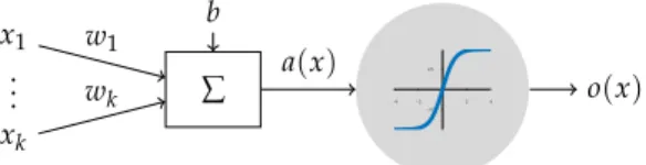
5.2 Neural networks ∑ −4 −2 2 4 −0.5 0.5 b .. . x1 xk w1 wk o(x) a(x)

Figure5.1:Neuron model .

feedforward NNs which do not contain cycles in the underlying graph. The restriction on feedforward NN simplifies the learning process. Furthermore, this architecture is sufficient for an arbitrary small approximation accuracy of the NN.

The neuron model

Each neuron is modeled with a simple scalar transfer functionσ:R→R, called the activation function. Appropriate choices for the activation function are e.g. σ(a) =sign(a),σ(a) = ( a a≥0 0 else ,σ(a) = 1 1+exp(−a).

The last one is a smooth approximation of the threshold functionσ(a) =

1

2(1+sign(a)). The input of a neuron consist of a weighted sum of the

outputs of all neurons connected to it. Furthermore, the input of each neuron can have additional biasbthat is added to the sum of weighted inputs. The outputoof the neuron is computed with the activation function as follows: o=σ( k

∑

wherewiare the edge weights andxiare the outputs of the previous neurons.

wiandbare the optimization variables in the learning task. A sketch of this

neuron model is given in Figure5.1. The network structure

We assume that the network is organized inΛlayers. Since we consider only feedforward NN, the outputs of the nodes of layeriare only connected

5 Approximation of the RMPC

to the inputs of the nodes of layeri+1. For simplicity, we consider fully connected feedforward NN. Fully connected means that each neuron of a layer has a connection to each neuron of the next layer. This simplifies the description of the network. The set of nodes can hence be decomposed into

Λdisjoint subsetsVi, i=1,...,Λ. The layer which produces the NN output

is called the output layer. All other layers are called hidden layers. In [35] the inputs are referred to as input layer and modeled as neuron. We omit this here as done in [36].

Each layerVihas a weight matrixWithat connects the outputs fromVi−1

to the inputs ofVi, a bias vector ¯biand an output vector ¯oi. Let theithlayer

consist ofjneurons. Therewith we can define the output vector ¯

oi=σ¯i(Wio¯i−1+b¯i),

of layerirecursively, where ¯ σi(x) =

h

σi,1(x1), ...,σi,j(xj)

i>

is the vector of the activation functionsσi,jof theithlayer and ¯o0is the NN

input. The NN output is ¯o_Λ. The activation ofViisAt= (Wio¯i−1+b¯i). As a

result, we get the network representation(V,E, ¯σ1,..., ¯σ_Λ,W1,...,WΛ,¯b1,...,¯bΛ).

Universal approximation

The following theorem guarantees that a NN satisfying any desired ap-proximation accuracy exists, if the RMPC output has only finitely many discontinuities. For the theorem, we need the following definition:

Definition17. A functionσis sigmoidal if

σ(a)→ 1 as t→+∞ 0 as t→ −∞ . (5.1)

Therewith, we can state the theorem as follows:

Theorem 18. [3] A feedforward network with only one hidden layer with sig-moidal activation functions and linear activation functions at the output layer can approximate any nonlinear function with finitely many discontinuities arbitrary well.

5.2 Neural networks

This is called the universal approximator theorem that yields a universal approximation property. Hence, we can find a NN that satisfies

πapprox(x)−πMPC(x)

_∞≤η,∀x∈ X_feas, (5.2) and thus guarantees stability and constraint satisfaction in combination with the RMPC for any choice ofη. However, to achieve a certain quality of approximation, a large amount of neurons and sampled input data may be necessary. Also, the optimal weights must be found what can be challenging in the optimization step.

5.2.2 Learning neural networks

In this subsection, we recap results for the learning of neural networks with supervised learning. This process is also often referred to as training.

The learning for NN has to be such, that it can be done in an automated fashion. Precomputed learning samples (x,πMPC(x)) can be used. The

widespread learning methods for NN are based on optimization using the gradient of a performance criterion with respect to parameters of the NN for some learning data. We recap in this section how the gradient can be computed for the mean squared error as performance function and how the gradient can be used for the optimization to achieve a NN with good performance.

To keep the learning effort tractable, we define the hypothesis setHby fixingV,E, and ¯σ1,..., ¯σ_Λbefore we start the gradient computation. Therefore,

(V,E, ¯σ1, ..., ¯σ_Λ)is called the architecture of the network [35]. We assume that the the RMPC algorithm has only finitely many discontinuities. Then an architecture with one sigmoidal hidden layer and a linear output layer can be sufficient to satisfy Assumption4for any choice of_η. Nevertheless, an

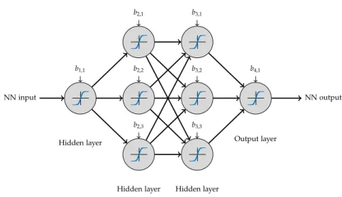
other network structure could be easier to learn. Often, multilayer networks can be learned faster and need less optimization parameters and hence less operations to evaluate them. This can also make it possible to use the resulting controller on cheap hardware. There is no general theory how to choose the optimal network structure. One possibility to derive the structure is Bayesian optimization (see e.g. [37] and [38]). Alternatively a line search can be used, if offline computational time requirements play a subordinate role. An example for a possible network structure is given in Figure5.2. The

remaining degrees of freedom if the network architecture is fixed are the weight matrices and biasW1,...,WΛ, ¯b1, ..., ¯bΛ. A certain choice of the weight

5 Approximation of the RMPC −4−2 24 −0.5 0.5 −4−2 24 −0.5 0.5 −4−2 24 −0.5 0.5 −4−2 24 −0.5 0.5 −4−2 24 − 0.5 0.5 −4−2 24 − 0.5 0.5 −4−2 24 − 0.5 0.5 −4−2 24 −0.5 0.5 NN input NN output Hidden layer

Hidden layer Hidden layer

Output layer b2,2 b1,1 b2,3 b2,1 b3,2 b3,3 b3,1 b4,1

Figure5.2:Example for a NN with three hidden layers.

matrices delivers one hypothesis from the hypothesis setH. A performance measure for the network is given by the mean squared error (mse), which is defined as mse(πapprox,D) = _Λ1 Λ

∑

The parameters W1, ...,WΛ,¯b1,...,¯bΛ are initialized randomly. Then the

network is learned by optimizing the values of weight matrices and bias to minimizing themsewhat enhances the network performance. To find good parametersW1, ...,WΛ,¯b1,...,¯bΛ, gradient based optimization can be used.

The gradient or respectively the Jacobi matrix of a NN can be computed with backpropagation [35, pp. 278-281]. With the resulting gradient, any standard numerical optimization can be used to learn the NN. Indeed there are some methods that have shown excellent performance for neural networks. A list of possible algorithms and benchmarks for algorithms are given in [36].

5.2 Neural networks

In [36] this issue is investigated by experiments on sample recursion and classification problems for different learning algorithms. Their result is that the Marquardt-Levenberg algorithm [39] delivers the smallest approximation error for regression problems and is hence especially suitable, if very accu-rate learning is required. This algorithm approximates Newton’s Method. Newton’s Method is a second order method and needs hence the Hessian matrix. The Marquardt-Levenberg algorithm approximates the Hessian ma-trix by the squared gradient of the NN. However, for networks with a large number of weights the Marquardt-Levenberg algorithm may be computa-tional inefficient since its computacomputa-tional effort increases geometrically. Then other algorithms like the scaled conjugate gradient algorithm [40] may be better.

We can spend some computational effort in learning the neural network and need an approximation error that satisfies a predefined bound. Fur-thermore, the RPI set Z_RPI of the RMPC algorithm gets smaller if the approximation error of the NN decreases. Hence it can be advantageous to spend more offline computation time for the learning to derive a better learned controller. Therefore we use the Marquardt-Levenberg algorithm. Now we discuss some details of how to facilitate the learning and to improve the approximation accuracy.

The learning of the NN is iteratively repeated until themseof the NN for a set of validation data, that is independent from the learning data set, begins to increase or until the difference of the performance between two iterations is below a user defined bound. Using the validation data ensures the avoidance of overfitting of the NN to the set of learning data.

Remark19. For systems with m multiple inputs, i.e. if u ∈ Rm_{, a NN can}

be computed for each input separately. This can have benefits in the learning. Furthermore, the computation of the AMPC feedback can then be parallelized by using m separate computation units.

Incremental learning and batch learning

There are different ways to learn NN [36]. One possibility is incremental learning, which updates the weights and biases at each time an input/output pair is presented to the network only for this pair. Another learning method is batch learning where the learning is performed after allΠ inputs and outputs for the network that shall be used for the learning are present at once. We focus in this thesis on batch learning. Incremental training

5 Approximation of the RMPC

may be necessary if the learning data exceeds the memory limits of the computer. Furthermore, depending on the used learning procedure, Mini Batch learning, where only a part of theΠsamples is used, may improve the learning performance. For details see e.g. [41].

Initializing the optimization parameters

Another important issue concerning the learning of NN is the initialization of the weights and biases. It can happen that the weights and biases of the network converge to a local but not global minimum [36]. In order to avoid such local minima and ensure a smaller approximation error, the learning procedure is started multiple times using random initial weights. This process is repeated until a NN with sufficiently small approximation error is found. The performance is validated with samples which are independent from the learning samples. If no such network can be found, the network architecture must be changed, e.g. using Bayesian optimization, or by using more learning samples (e.g. created by a more dense sampling).

Preprocessing

The performance of the NN learning can be enhanced by preprocessing and postprocessing steps [36]. If sigmoidal transfer functions are used, the activation of a neuron becomes saturated for a large input. Then, the gradient gets small, which causes a slow learning. To avoid this, a preprocessing step can be performed to normalize the input and output of the supervised learning problem. We normalize the neural NN inputs as well as the NN outputs such that the learning data falls in the range of[−1,1]. For details on preprocessing and more complex methods see e.g. [36].

Sampling the RMPC algorithm

To learn a NN, we need learning data that contains enough information about the control law πMPC on the whole feasible set of the MPC. This

learning data can be obtained by sampling the RMPC.

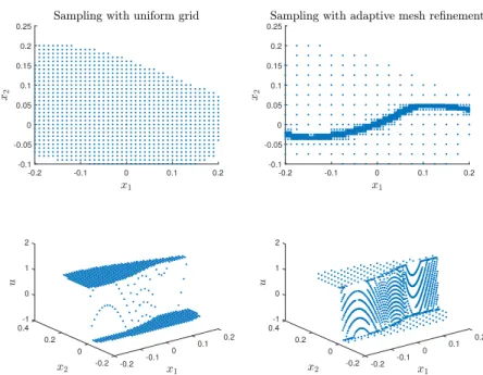
One simple possibility is sampling with a uniform grid. The question that arises is how dense this grid needs to be. To keep the computational effort tractable, it is important to sample not with too high resolution. In general the question for the optimal density is hard to answer and depends heavily on the system to control. The density can be estimated empirically by

5.2 Neural networks -0.2 -0.1 0 0.1 0.2 -0.1 -0.05 0 0.05 0.1 0.15 0.2 0.25 -0.2 -0.1 0 0.1 0.2 -0.1 -0.05 0 0.05 0.1 0.15 0.2 0.25 -1 0.4 0 0.2 0.2 1 0.1 2 0 0 -0.1 -0.2 -0.2 -1 0.4 0 0.2 0.2 1 0.1 2 0 0 -0.1 -0.2 -0.2

Figure5.3:Comparison of different sampling strategies for the numerical example from Chapter7.

trying to learn the MPC algorithm for a small region with several different densities and to choose the sparsest density for which a NN that satisfies Assumption4can be found.

Another sampling strategy is adaptive mesh refinement. For this strategy, the setX is divided into a user defined number of polytopes of the same size. The RMPC is sampled for all corner points of the polytope. If the output error between two corner points exceeds a user defined bound, the polytope is partitioned inton2smaller polytopes of equal size. The aim of this strategy is to decrease the number of required samples. It has resemblances to [42]. A comparison for adaptive mesh refinement and a uniform grid is given in Figure5.3, in which both strategies are used with the same number of total

samples for an example system. Note that infeasible samples are discarded for both methods.