University of Massachusetts Amherst University of Massachusetts Amherst
ScholarWorks@UMass Amherst
ScholarWorks@UMass Amherst
Doctoral Dissertations Dissertations and Theses
July 2016
Effective Performance Analysis and Debugging
Effective Performance Analysis and Debugging
Charles M. CurtsingerFollow this and additional works at: https://scholarworks.umass.edu/dissertations_2
Part of the OS and Networks Commons, and the Programming Languages and Compilers Commons
Recommended Citation Recommended Citation
Curtsinger, Charles M., "Effective Performance Analysis and Debugging" (2016). Doctoral Dissertations. 632.
https://scholarworks.umass.edu/dissertations_2/632
This Open Access Dissertation is brought to you for free and open access by the Dissertations and Theses at ScholarWorks@UMass Amherst. It has been accepted for inclusion in Doctoral Dissertations by an authorized administrator of ScholarWorks@UMass Amherst. For more information, please contact
EFFECTIVE PERFORMANCE ANALYSIS AND DEBUGGING
A Dissertation Presented by
CHARLES M. CURTSINGER
Submitted to the Graduate School of the
University of Massachusetts Amherst in partial fulfillment of the requirements for the degree of
DOCTOR OF PHILOSOPHY May 2016
© Copyright by Charles M. Curtsinger 2016 All Rights Reserved
EFFECTIVE PERFORMANCE ANALYSIS AND DEBUGGING
A Dissertation Presented by
CHARLES M. CURTSINGER
Approved as to style and content by:
Emery D. Berger, Chair
Yuriy Brun, Member
Arjun Guha, Member
Nicholas G. Reich, Member
James Allan, Chair
DEDICATION
ACKNOWLEDGEMENTS
First, I would like to thank my advisor, Emery Berger, for his support during my graduate career. Your advice and mentoring shaped every element of this dissertation, and your tireless advocacy for me have shaped my entire career. None of this would have been possible without you. Thank you.
Thanks as well to my fellow students Gene Novark, Tongping Liu, John Altidor, Matt Laquidara, Kaituo Li, Justin Aquadro, Nitin Gupta, Dan Barowy, Emma Tosch, and John Vilk. You took the daunting process of spending over half a decade working seemingly endless hours and made it truly fun. I hope I have helped you with your work as much as you helped me with mine.
I would also like to thank my research mentors and colleagues Steve Freund, Yannis Smaragdakis, Scott Kaplan, Arjun Guha, Yuriy Brun, Ben Zorn, Ben Livshits, Steve Fink, Rodric Rabbah, and Ioana Baldini. Your guidance and support over the years have been an enormous help, and it has been a real privilege to work with you all.
Finally, I would like to thank my parents Jim and Julie, my brother Dan, my wife Nikki, and parents in-law Kathy and Cary, for their unwavering support and understanding. Thank you for your constant encouragement, for listening to the long technical explanations you may or may not have asked for, and for tolerating all the weekends and holidays I spent working instead of spending time with you. I could never have finished a PhD without your support and encouragement.
ABSTRACT
EFFECTIVE PERFORMANCE ANALYSIS AND DEBUGGING MAY 2016
CHARLES M. CURTSINGER B.Sc., UNIVERSITY OF MINNESOTA
M.Sc., UNIVERSITY OF MASSACHUSETTS AMHERST Ph.D., UNIVERSITY OF MASSACHUSETTS AMHERST
Directed by: Professor Emery D. Berger
Performance is once again a first-class concern. Developers can no longer wait for the next gen-eration of processors to automatically “optimize” their software. Unfortunately, existing techniques for performance analysis and debugging cannot cope with complex modern hardware, concurrent software, or latency-sensitive software services.
While processor speeds have remained constant, increasing transistor counts have allowed architects to increase processor complexity. This complexity often improves performance, but the benefits can be brittle; small changes to a program’s code, inputs, or execution environment can dramatically change performance, resulting in unpredictable performance in deployed software and complicating performance evaluation and debugging. Developers seeking to improve performance must resort to manual performance tuning for large performance gains. Software profilers are meant to guide developers to important code, but conventional profilers do not produce actionable information for concurrent applications. These profilers report where a program spends its time, not where optimizations will yield performance improvements. Furthermore, latency is a critical measure of performance for software services and interactive applications, but conventional profilers measure only throughput. Many performance issues appear only when a system is under high load,
but generating this load in development is often impossible. Developers need to identify and mitigate scalability issues before deploying software, but existing tools offer developers little or no assistance.
In this dissertation, I introduce an empirically-driven approach to performance analysis and
debugging. I present three systems for performance analysis and debugging. STABILIZERmitigates
the performance variability that is inherent in modern processors, enabling both predictable
perfor-mance in deployment and statistically sound perforperfor-mance evaluation. COZconductsperformance
experimentsusingvirtual speedupsto create the effect of an optimization in a running application. This approach accurately predicts the effect of hypothetical optimizations, guiding developers to
code where optimizations will have the largest effect. AMPallows developers to evaluate system
scalability usingload amplificationto create the effect of high load in a testing environment. In
combination, AMPand COZallow developers to pinpoint code where manual optimizations will
TABLE OF CONTENTS
Page
ACKNOWLEDGEMENTS. . . v
ABSTRACT . . . .vi
LIST OF TABLES. . . xii
LIST OF FIGURES . . . .xiii
CHAPTER 1. INTRODUCTION . . . 1 1.1 Performance Measurement. . . 1 1.2 Performance Profiling. . . 2 1.3 Performance Prediction. . . 2 1.4 Contributions . . . 2
1.4.1 STABILIZER: Predictable and Analyzable Performance . . . 2
1.4.2 COZ: Finding Code that Counts with Causal Profiling . . . 3
1.4.3 AMP: Scalability Prediction and Guidance with Load Amplification . . . 3
2. BACKGROUND . . . 5
2.1 Software pre–1990 . . . 5
2.1.1 The Batch Execution Model . . . 5
2.1.2 Interactive Computation . . . 6 2.2 Hardware pre-1990 . . . 6 2.2.1 Performance Variability . . . 7 2.3 Measuring Performance . . . 8 2.4 Improving Performance . . . 9 2.4.1 Compilation . . . 9 2.4.2 Software Profilers . . . 12
3. CHALLENGES IN PERFORMANCE ANALYSIS AND DEBUGGING. . . 15
3.1 Unpredictable Performance . . . 15
3.1.1 Causes of Performance Unpredictability . . . 16
3.1.2 Challenges for Performance Evaluation . . . 17
3.1.3 Challenges for Software Deployment . . . 18
3.2 Limitations of Software Profilers . . . 19
3.2.1 Concurrency . . . 19
3.2.2 Throughput and Latency . . . 20
3.3 Building Scalable Software . . . 21
4. STABILIZER: PREDICTABLE AND ANALYZABLE PERFORMANCE. . . 23
4.0.1 Contributions . . . 24
4.1 Overview . . . 25
4.1.1 Comprehensive Layout Randomization . . . 25
4.1.2 Normally Distributed Execution Time . . . 25
4.1.3 Sound Performance Analysis . . . 26
4.1.4 Evaluating Code Modifications . . . 26
4.1.5 Evaluating Compiler and Runtime Optimizations . . . 27
4.1.6 Evaluating Optimizations Targeting Layout . . . 27
4.2 Implementation . . . 27
4.2.1 Building Programs with Stabilizer . . . 28
4.2.2 Heap Randomization . . . 28
4.2.3 Code Randomization . . . 30
4.2.4 Stack Randomization. . . 32
4.2.5 Architecture-Specific Implementation Details . . . 33
4.3 Statistical Analysis . . . 34
4.3.1 Base case: a single loop . . . 34
4.3.2 Programs with phase behavior . . . 35
4.3.3 Heap accesses . . . 36
4.4 Evaluation . . . 36
4.4.1 Benchmarks . . . 36
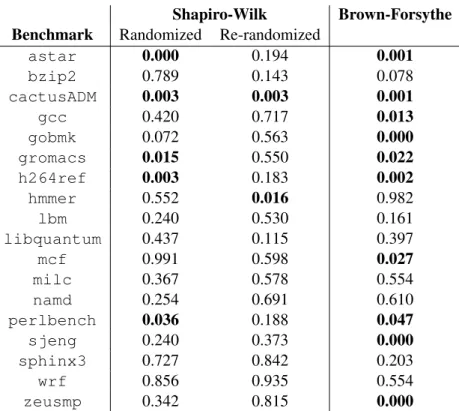
4.4.2 Normality . . . 37
4.4.3 Efficiency . . . 38
4.5 Sound Performance Analysis . . . 41
4.6 Conclusion . . . 43
5. COZ: FINDING CODE THAT COUNTS WITH CAUSAL PROFILING. . . 44
5.0.1 Contributions . . . 46
5.1 Causal Profiling Overview . . . 46
5.1.1 Profiler Startup . . . 47
5.1.2 Experiment Initialization . . . 47
5.1.3 Applying a Virtual Speedup . . . 47
5.1.4 Ending an Experiment . . . 48
5.1.5 Producing a Causal Profile . . . 48
5.1.6 Interpreting a Causal Profile . . . 49
5.2 Implementation . . . 50
5.2.1 Core Mechanisms . . . 50
5.2.2 Performance Experiment Implementation . . . 51
5.2.3 Progress Point Implementation . . . 52
5.2.4 Virtual Speedup Implementation . . . 53
5.2.5 Implementing Virtual Speedup with Sampling . . . 54
5.3 Evaluation . . . 59 5.3.1 Experimental Setup . . . 59 5.3.2 Effectiveness . . . 59 5.3.3 Accuracy . . . 67 5.3.4 Efficiency . . . 68 5.4 Conclusion . . . 70
6. AMP: SCALABILITY PREDICTION AND GUIDANCE WITH LOAD AMPLIFICATION. . . 71
6.0.1 Contributions . . . 74
6.1 Design and Implementation . . . 74
6.1.1 Using AMP. . . 74
6.1.2 Amplifying Load with Virtual Speedup . . . 75
6.1.3 Implementation . . . 76
6.2 Causal Profiling with Amplified Load . . . 77
6.3 Evaluation . . . 78
6.3.1 Case Study: Ferret . . . 79
6.3.2 Case Study: Dedup . . . 80
6.4 Conclusion . . . 83
7. RELATED WORK. . . 84
7.1 Performance Evaluation . . . 84
7.2 Program Layout Randomization . . . 85
7.2.1 Randomization for Security . . . 85
7.2.2 Predictable Performance . . . 86
7.3 Software Profiling . . . 86
7.3.1 General-Purpose Profilers . . . 86
7.3.2 Parallel Profilers . . . 87
7.3.3 Performance Guidance and Experimentation . . . 88
7.4 Scalability and Bottleneck Identification . . . 88
7.4.1 Profiling for Parallelization and Scalability . . . 89
8. CONCLUSION . . . 90
LIST OF TABLES
Table Page
4.1 Normality and variance results for SPEC CPU2006 benchmarks run with
STABILIZERusing one-time and repeated randomization . . . 37
5.1 POSIX functions that COZintercepts to handle thread wakeup . . . 56
5.2 POSIX functions that COZintercepts to handle thread blocking . . . 56
5.3 Results for benchmarks optimized using COZ. . . 59
5.4 Summary of progress points and causal profile results for the remaining PARSEC benchmarks . . . 67
LIST OF FIGURES
Figure Page
3.1 A simple multithreaded program that illustrates the shortcomings of existing
profilers . . . 20
3.2 A gprof profile for the program in Figure 3.1 . . . 20
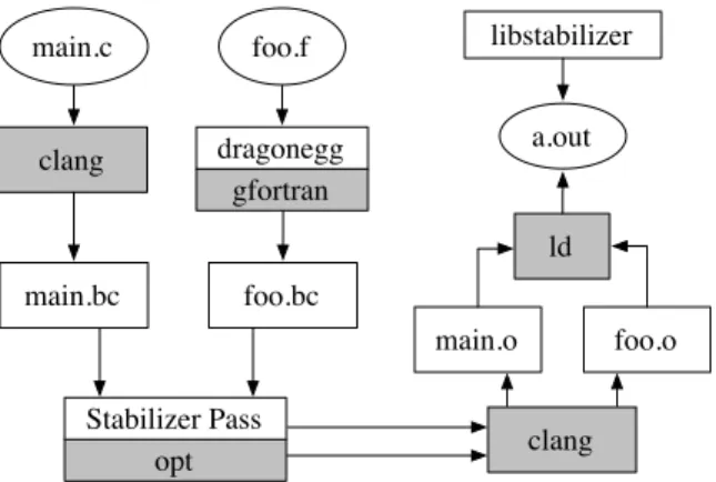
4.1 The procedure for building a program with STABILIZER. . . 28
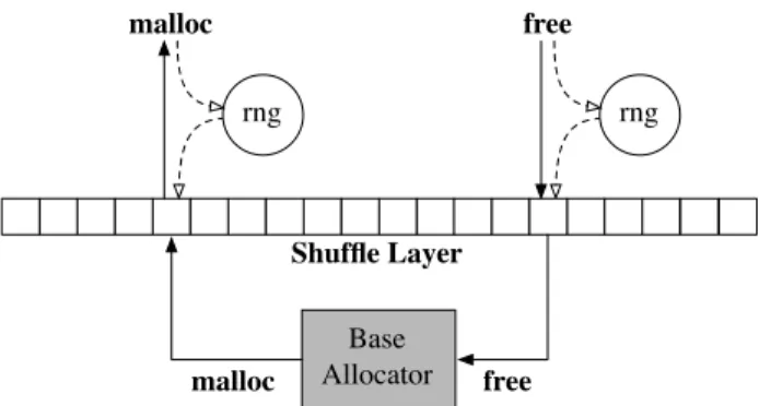
4.2 An illustration of STABILIZER’s heap randomization . . . 29
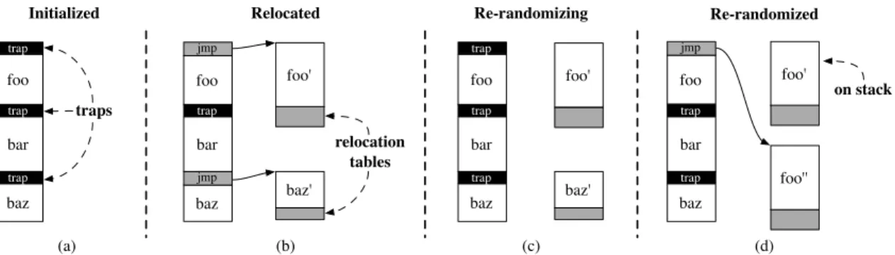
4.3 An illustration of STABILIZER’s code randomization . . . 30
4.4 An illustration of STABILIZER’s stack randomization . . . 33
4.5 Quantile-quantile plots showing the distributions of execution times with STABILIZER. . . 39
4.6 Distribution of runtimes with STABILIZERone-time and repeated randomization . . . 40
4.7 Speedup of-O2over-O1, and-O3over-O2optimizations in LLVM . . . 42
5.1 A simple multithreaded program that illustrates the shortcomings of existing profilers . . . 45
5.2 A causal profile forexample.cpp, shown in Figure 5.1 . . . 45
5.3 An illustration of virtual speedup . . . 48
5.4 Hash function performance in dedup . . . 60
5.5 An illustration of ferret’s pipeline . . . 61
5.6 COZoutput for the unmodified ferret application . . . 63
5.7 Causal profile for SQLite . . . 63
5.8 A conventional profile for SQLite, collected using the Linux perf tool . . . 64
5.10 Percent overhead for each of COZ’s possible sources of overhead . . . 68
6.1 A simple multithreaded program with a scalability issue that will not appear in testing . . . 72
6.2 Scalability measurements for the program in Figure 6.1 . . . 73
6.3 AMP’s scalability predictions for the program in Figure 6.1 . . . 74
6.4 The real effect of speeding up consumers in the program from Figure 6.1 . . . 78
6.5 The effect of speeding up consumers in the program from Figure 6.1 . . . 79
6.6 AMP’s scalability predictions for ferret, after incorporating optimizations from Chapter 5 . . . 80
6.7 The causal profile results for the ranking stage in ferret with and without load amplification . . . 80
6.8 AMP’s scalability predictions for dedup, after incorporating optimizations from Chapter 5 . . . 81
6.9 Load-amplified causal profile results forencoder.c:102in dedup . . . 81
6.10 Load-amplified causal profile results forrabin.c:110in dedup . . . 82
CHAPTER 1 INTRODUCTION
Developers can no longer count on increasing processor speed to automatically “optimize” their programs; performance must be a first-class concern. Unfortunately, the tools and practices supporting software performance have been neglected during decades of exponential growth in processor performance. During the last three decades, we have moved from a model of batch execution on relatively simple processors to massively-parallel software services running on processors with billions of components. These changes make it nearly impossible to reliably measure, predict, and debug performance using techniques from the 1980s and earlier. In this dissertation, I introduce three novel software performance tools that enable reliable performance measurement, effective performance debugging, and accurate performance prediction.
1.1 Performance Measurement.
Clock speed is an important factor in determining a processor’s performance, but it is by no means the only one. The speed of memory accesses has not kept pace with clock speed increases, so processors now rely on complex heuristics like caching and prefetching to hide the latency of memory accesses. When these heuristics work well, processors run orders of magnitude faster than they would without them. However, caches are have undesirable edge cases that lead to significant performance degradations. Tiny changes in the placement of a program’s code or data in memory can have catastrophic effects on performance. This makes it particularly difficult to compare the performance of two versions of a program. Programs with different algorithms almost certainly have different layouts as well; if one version runs faster than the other, is the root cause the new algorithm or the layout change? The confounding effect of program layout can lead developers to make poor decisions during performance evaluation, but can also lead to unpredictable performance of deployed software.
1.2 Performance Profiling.
Processor clock speeds have remained relatively constant for the last ten years. While larger caches and improvements in processor design still help improve the performance of new processors, the year-over-year improvements are small. As a result, developers must now resort to manual performance tuning to improve the performance of their code. Software profilers are designed to help developers decide where to focus during manual performance tuning. Unfortunately, existing profilers do not provide actionable information for concurrent programs; they only report where programs spend their time, not where performance improvements would reduce end-to-end runtime or latency in a parallel program. This leads developers to pursue manual optimizations with little or no potential payoff.
1.3 Performance Prediction.
The era of batch computation is long gone; instead, computational workloads are now dominated by service-oriented software. These services must scale to thousands or millions of concurrent requests while remaining responsive, or they can bring down an entire network of applications. This makes performance testing particularly critical. However, generating sufficient load in testing infrastructure is often impractical or impossible, and existing performance analysis and debugging techniques do not help developers identify code that limits scalability. Developers are left with only one option: deploy software with inadequate performance testing. When performance bugs inevitably appear in production, developers have no means to reproduce and investigate these bugs in the development environment.
1.4 Contributions
This dissertation presents three systems that support a new approach to performance analysis and debugging. Collectively, these systems enable reliable performance measurement, effective performance debugging, and accurate performance prediction.
1.4.1 STABILIZER: Predictable and Analyzable Performance
Developers use performance measurements to decide whether a code change has unacceptable performance overhead, or whether an optimization significantly improves performance. However,
standard performance evaluation strategies are measuring more than just the effect of the code change; any change to a program’s code also changes its layout, which can have a large effect on performance that obscures the real cost or benefit of code changes. Repeated executions of the program do not control for the performance effect of layout; every run executes with the same memory layout, so layout changes produce a consistent bias in experimental results. This dissertation
presents STABILIZER, a system that controls for the effect of memory layout using randomization,
and presents an representative performance evaluation of compiler optimizations performed with STABILIZERand sound statistical methods.
1.4.2 COZ: Finding Code that Counts with Causal Profiling
Developers need to know which parts of an application are important for performance; they use this information to select code for manual performance tuning, or to determine which code should be left undisturbed when adding new features that could impose runtime overhead. To find performance-critical code, developers must consider all dependencies and sources of contention between an application’s concurrently-executing tasks. Existing tools for identifying performance critical code, software profilers, produce misleading results because they do not consider the complex interactions between tasks in concurrent programs. Existing software profilers, which typically measure the amount of time spent executing each of a program’s functions, fail to answer developers’ primary
question:where will optimizations have the largest effect on program performance?This dissertation
presentscausal profiling, a novel profiling technique that simulates the effect of optimizations to
specific code fragments to empirically establish the potential benefit of a real optimization. Using
COZ, a prototype causal profiler, I identify optimization opportunities in Memcached, SQLite, and
the PARSEC benchmarks that lead to program speedups as large as 68%, and show that the effects of
these optimizations match COZ’s predictions.
1.4.3 AMP: Scalability Prediction and Guidance with Load Amplification
The growth in high performance software services poses a problem for performance evaluation and debugging. These systems are designed to handle enormous load—significantly more load than can be generated on a single test machine. Developers have no means to test these systems under realistic loads before deployment. As a result, performance issues may lie dormant in an application
until it is deployed. This dissertation presents AMP, a system that simulates the effect of higher
load in a running program withload amplification, and directly measures the system performance
under the simulated load. In combination with COZ, AMPcan be used to precisely locate code where
CHAPTER 2 BACKGROUND
While processor designs and software architectures have changed dramatically since the 1980s, the key ideas in software performance are at least this old. This chapter introduces the basics of software and hardware pre-1990 and the techniques for performance analysis and debugging from this area, which largely remain in use today.
2.1 Software pre–1990
Before the era of personal computers, the vast majority of programs were run abatch jobs, where
end-to-end runtime was all that mattered. On early computers, batch jobs executed in isolation with near-complete control over a machine and all of its resources. As computers grew in computational power, multi-user systems became common; these machines maintained the illusion of exclusive control of all resources, but hardware resources were actually multiplexed over all users’ jobs to execute many independent tasks in parallel. This usage model continued through the 1980s on minicomputers, which displaced large mainframes.
2.1.1 The Batch Execution Model
Batch jobs lend themselves to a simple model of performance; because each job must complete before the next can be run, runtime is additive. If a system has three jobs to execute, saving a minute on any of the three jobs would shorten the total runtime by one minute. It does not matter where this saved minute comes from, the effect is the same.
In the multi-user model, different users can execute batch jobs concurrently. While multi-user machines share the resources of a single machine between many concurrently executing tasks, these tasks were almost entirely independent. Communication between different users’ computations were rare or impossible, depending on the hardware and operating system. As a result, batch jobs
executed by one user resemble batch jobs executed in isolation on a less-powerful machine. The simple performance model for a single-user machine remains useful for multi-user machines as well.
2.1.2 Interactive Computation
While batch computation dominated on high performance machines, an alternative model— interactive computation—was growing in use, especially on personal computers. Rather than churning on data until a result is available, interactive applications perform computation in response to user inputs that occur during normal execution rather than just at the beginning. A spreadsheet application from this era would be considered an interactive application, but its computational model
is remarkable similar to batch computation. The program runs in anevent loop, which repeatedly
checks for user input. Once a user has updated a cell or formula the program initiates a recalculation (effectively a batch computation). The program will not respond to any additional inputs until after the recalculation is complete and the program can resume executing the event loop. To improve the responsiveness of a spreadsheet application a developer simply needs to reduce the execution time of the recalculation, which is effectively a batch computation run in response to user input.
2.2 Hardware pre-1990
The additive property of software runtimes extended to the hardware level as well. Programs are composed of instructions, which a processor must execute in order. Executing an instruction requires several steps:
1. fetch the instruction from the computer’s main memory; 2. decode the instruction from its in-memory representation;
3. collect the instruction’s inputs from memory and registers, a limited set of locations used to store values that will be needed quickly;
4. perform the operation specified by the instruction; and finally, 5. place the result(s) of the instruction in registers or memory.
Early processors performed each operation in sequence for one instruction before moving on to the next one. While the execution times of some steps in instruction execution could vary, the time to
run a single instruction from start to finish was often tied to a clock with a period long enough to
allowanyinstruction to complete in the allotted time.
By the 1970s, many computers usedpipelined execution to increase instruction throughput.
Rather than performing all of the steps in instruction execution for a single instruction before moving on to the next instruction, a pipelined processor executes multiple instructions concurrently in stages. At any given point, a pipelined processor can be fetching one instruction, decoding another, collecting inputs for a third, and so on. The net effect of this change is improved performance, but the time required to execute a single instruction is just as predictable as in the non-pipelined model.
2.2.1 Performance Variability
Software performance was not entirely consistent; one early source of performance variability in early computers was in memory accesses. Many computers used inexpensive rotating drum memory; the storage was spread across a two dimensional area wrapped around a cylinder with a reading head spanning the length of the cylinder. An entire row of memory (the length of the cylinder) could be read at once, but reading along the circumference would require rotating the drum until the desired row was under the read head. The time required to load from drum memory depends on the distance between the current head location and the target column. A common practice among programmers seeking to optimize programs was to carefully plan memory use so the drum would already be rotated into place when a row of memory was needed. This level of control allowed careful developers to eliminate a source of unpredictability in performance through careful design and a deep understanding of the underlying hardware.
While rotating drum memory was largely displaced by core memory (which has no moving parts) by 1960, this view of hardware performance as a predictable outcome applied equally well to newer memory systems and processors designs until the 1990s. As a result, much of the work on measuring and improving performance is built on two core assumptions:
1. A program interacts with hardware in predictable, controllable ways, and
2. runtime is additive. In other words, a program’s total runtime is the sum over the execution time of all its parts.
While reasonable at the time, these assumptions no longer hold; interactions between complex hardware components make performance virtually impossible to predict. Despite this fact, the practices in software performance engineering developed during this era remain in use today.
2.3 Measuring Performance
Measuring the performance of a program seems like a straightforward process; start a timer, run the program, then stop the timer. There are, of course, additional details that must be addressed:
1. How should time be measured to ensure the most accurate measurement?
2. What operations could the system perform that may distort the program’s runtime, and how can these be disabled or accounted for?
3. What inputs should the program be given?
Answers to these questions are largely system- and program-dependent, but coming up with answers is not especially challenging. Some care was required to time the program accurately, but the majority of the effort in evaluating a program’s performance went toward choosing representative inputs. If real inputs to a program exercise parts of the code that are not used during performance evaluation, developers may miss important opportunities to improve performance. Producing representative inputs requires collecting program inputs that will result in the same parts of the program running for approximately the same time as under real workloads.
Evaluating the performance of application-independent systems such as a new processor archi-tecture, operating system, or runtime library adds one dimension of complexity to performance evaluation. These systems impact the performance of different programs in different ways, so which programs should be run to test the system’s performance? There have been efforts to address this issue with the development of standard benchmark suites, although the selection of programs, inputs, and performance measures for benchmark suites can be controversial [69, 31]. Debates over which benchmark applications should be included, the inputs used to drive these applications, and the type of mean used to summarize results were and are still common. However, the implications for developers were minimal; given an application and representative inputs, developers could easily evaluate the performance of a new processor, operating system, or version of the application.
2.4 Improving Performance
There are both automatic and manual techniques for improving software performance. Automatic
performance improvements largely come fromcompiler optimizations, which transform the structure
of a program while maintaining semantic equivalence to the original program. Developers can manually improve a program’s performance by changing algorithms and data structures, the input and output formats, and other high-level design decisions that require application-specific knowledge.
Manual performance improvements require significant developer effort, so they often rely onsoftware
profilersto identify code that is important enough to justify manual effort. This section introduces the basic methods of automatic performance improvements with compiler optimizations, the mechanisms used by software profilers, and how software profiles are interpreted.
2.4.1 Compilation
Compilers are responsible for transforming code in a high level language to instructions the processor can execute. This process contains three major steps:
1. Translation to intermediate representation (IR).In this phase of compilation, often called the “front-end,” high level syntax is parsed and transformed to an intermediate representation. This intermediate representation is designed to be amenable to analysis, transformation, and generation of the final machine code. While important, this step typically does not impact the performance of the final executable file.
2. Analysis and transformation.Once a program has been translated to IR, the compiler ana-lyzes the IR and applies transformations to improve the performance of the final executable. These transformations fall under the general category of “optimizations,” although the result is not necessarily optimal. This phase is sometimes referred to as the “middle-end” of the compiler.
3. Code generation.Once the compiler has completed transformations, the “back-end” is re-sponsible for translating IR to machine-executable code. Two major components of this phase include register allocation, which assigns program variables in the IR to registers, a limited set of “variables” available on a processor; and instruction selection, the process of determining exactly which hardware instruction(s) should be used to to carry out an operation or sequence
of operations in the program’s intermediate representation. Strategies for register allocation, instruction selection, and other aspects of code generation play an important role in program performance.
2.4.1.1 Compiler Optimizations
Transformations to a program’s intermediate representation and strategies for code generation can have a significant impact on the program’s performance. However, these strategies are ultimately just heuristics tailored to specific properties of a target processor architecture. While the details of many optimizations are highly technical or processor-dependent, many optimizations are common to most processors. Optimizations are generally organized into levels, where selecting a level enables
an entire group of optimizations. Compilers generally use the command line flag-Oto specify
the optimization level. The-O0 flag enables only the most basic strategies for code generation,
-O1enables only a few simple transformations,-O2(usually the default) applies a standard suite
optimizations, and-O3applies “advanced” optimizations that are often computationally expensive or
deemed experimental. Some compilers include additional levels of optimization such as-O4, which
runs the program to collect dynamic information which is then used to guide transformations, and
-Os, which targets a smaller executable by enabling only the transformations that do not increase
executable size. Thegcccompiler generously accepts optimization levels of five and above, but
the effect is the same as passing in the-O4option. This subsection briefly introduces a few of
these optimizations to give a sense of what a compiler can and cannot do to improve performance automatically.
2.4.1.1.1 Constant Folding & Propagation. Compilers often use an intermediate representation in what is called single static assignment (SSA) form. In this form, variables are assigned at their declarations, and cannot be re-assigned. This simplifies the task of determining the set of possible values for a variable at any given point. The value may be a constant, the result of some other instruction, or a load from memory. Constant folding locates operations that are always given constant values as inputs and replaces the operation with its result. This eliminates an instruction from the IR—and most likely a machine instruction as well—and creates a new constant value that could potentially be used in another round of constant folding. Constant propagation complements
this transformation by replacing variables that are known to contain constant values with the constant itself, enabling further folding and propagation.
2.4.1.1.2 Common Subexpression Elimination. The aptly named “common subexpression elimination” optimization identifies and eliminates repeated calculations of the same value. By computing an intermediate result and storing it in an IR variable, multiple operations that use this value can share the result rather than recomputing it. Unlike constant folding and propagation, this transformation is suitable for values that are unknown at compile time such as program inputs, values loaded from memory, or values that depend on computations that use unknown values.
2.4.1.1.3 Function Inlining. Function inlining takes calls from one function (the caller) to an-other (the callee), and replaces the function call by embedding the body of the callee function directly in the caller. This eliminates the modest overhead of making a function call, but the value in function inlining is largely in enabling other optimizations. If a function is called with constants as arguments, inlining the function allows constant folding and propagation to cross the function boundary, effectively specializing the inlined function for this callsite.
2.4.1.1.4 Loop Unrolling. Many program optimizations target loops, which necessarily make up a significant portion of a program’s execution. A program with two billion instructions, a very large number even for complex software such as an operating system, would run for just one second on a 2GHz processor if it did not contain loops.
Loops are implemented using conditional branches in both IR and machine code; these languages
do not have high-level control constructs likeifstatements orwhileloops. Before each iteration
of a loop, the program executes a conditional branch, which jumps to a specific program point only if some value meets a condition (e.g. “jump to LABEL if x is less than 10”). The performance cost of a single conditional branch is very small, but loops that run for thousands of iterations will execute thousands of conditional branches. Loop unrolling takes the body of the loop and replaces it with a new body that executes multiple iterations in sequence, dividing the number of conditional branches
by some constant. One goal of loop unrolling is to fit the loop body into a singlecache line, the size
of caches). Given this upper limit, most compilers unroll loops so each new iteration will execute between two and eight iterations of the original loop.
2.4.1.1.5 Strength Reduction. Strength reduction identifies special cases of expensive operations— often multiplication or division—and translates them into less-expensive operations. For example, a processor can multiply an integer by two by simply adding a zero to the right side of the number in binary representation; this is the same as multiplying a decimal number by ten by simply adding a zero. This operation, called a left shift, is much less expensive than full multiplication but achieves the same result.
The specifics of strength reduction are often processor-dependent. As an example, the x86
architecture includes theleainstruction, which multiplies one value by a constant, then adds the
result to another value. This instruction was originally meant for computing the address of elements in an array, but works equally well for computation; in many versions of the x86 architecture, the
time to execute anleainstruction is less than the time required to multiply a value by a constant
and complete an add instruction [1].
2.4.2 Software Profilers
Once the benefit of compiler optimizations has been exhausted, developers are left to manually change code in the hope of improving performance. These changes often require higher-level decisions such as which algorithm to use, how to design a file for quick access, and other application-specific factors that cannot be managed automatically. These changes are often invasive, requiring significant intellectual and implementation effort; it is infeasible for developers to try changing every piece of a large system, so they rely on software profilers to identify important code. Conventional profilers are generally implemented using instrumentation, sampling, or a combination of both.
2.4.2.1 Instrumentation-based Profilers
Instrumentation-based profilers monitor a program’s execution by inserting tracking code using the compiler. When the program is run, this monitoring code records the behavior of the program and the time between events. The collected information often includes the time required to execute a function and the number of times it was called. One issue with instrumentation-based profilers isprobe effect; the time to execute tracking code distorts the program’s runtime. If probe effect is
particularly large, the profiler ends up measuring performance characteristics of the instrumentation rather than the original program. As a result, virtually no profilers use instrumentation exclusively, and many do not use it at all.
2.4.2.2 Sampling-based Profilers
Rather than instrumenting a program and monitoring every step of its execution, sampling-based or statistical profilers periodically pause a running program and record its state. Each time a sampling profiler pauses the program, it determines which function is currently executing. The number of samples in a particular function is approximately equal to the fraction of program runtime spent in that function. Sampling profilers can also examine the program’s call stack to break down time spent in a function based on where it was called from. While sampling profilers necessarily admit some amount of error, they are generally more accurate than instrumentation-based profilers because they have very little probe effect. Unfortunately, there is no reliable way to count invocations of a function using this type of sampling, only the time spent in a particular function.
2.4.2.3 Hybrid Profilers
Hybrid profilers use sampling to collect as much information as possible, while relying on instrumentation to gather information that cannot be measured using sampling. The canonical example is gprof, which uses sampling to measure time spent in each function but also inserts instrumentation to count invocations of each caller–callee pair [33]. This additional information is
used to construct acall graph, which shows the number of times each function was called from each
callsite, and how long these invocations took on average. By tracking execution time with sampling, gprof has much lower overhead than it would be if timer code was included in the instrumentation.
2.4.2.4 Interpreting a Software Profile
Profilers typically measure two quantities: the amount of time spent in a particular function, and the number of times that fragment was executed. When every piece of a program is run in sequence, this information leads developers to good targets for optimizations. If a function contributes very little to total execution time, then optimizing it will not have a large effect on total runtime. Conversely, the number of times a function is executed serves to multiply the benefits of a small performance
improvement; reducing the runtime for a function that runs one million times by just 3.6 milliseconds will reduce total runtime by one hour. Unfortunately, more recent architecture, software designs, and usage models make conventional profilers much less useful.
2.4.2.5 Extensions of Software Profiling
Much of the work on software profilers has focused on collecting as much information as possible with minimal probe effect. A sampling-based profiler that pauses execution after some number of clock ticks will collect a number of samples roughly proportional to the execution time spent in a function. Likewise, pausing a program after some number of other events can roughly determine
what fraction of those events occurred in a particular function. For example, sampling every n
memory accesses allows a developer to see approximately what fraction of total memory accesses are issued by each function. Sampling on a variety of hardware events is available in both the perf and oprofile sampling-based profilers [46, 51]. While these approaches sometimes show surprising performance results, it generally not clear how to reduce the number of memory accesses or some other performance-degrading hardware event in a particular function.
Other profiling techniques have been developed to monitor time programs spend waiting for inputs or computation, to identify code that is amenable to parallelization, or to trace program paths; see Chapter 7 for a full discussion of other profiling techniques.
CHAPTER 3
CHALLENGES IN PERFORMANCE ANALYSIS AND DEBUGGING
Performance analysis and debugging remains a significant challenge, despite decades of work on measuring, understanding, and improving software performance. Modern processors designs often lead to good performance, but “unlucky” inputs or code changes can lead to significant performance regressions. As a result, performance is highly unpredictable and thus difficult to measure accurately. Software profilers are designed to help developers identify code where manual performance tuning would improve whole-program performance, but existing profilers are not well-suited to concurrent software or modern performance concerns. Scalability is a primary concern in software performance; developers must evaluate system in a test environment, but the load conditions in test may not expose scalability bottlenecks that will show up in deployment. Testing systems under realistic load is often impractical or impossible. Just as profilers do not lead developers to code that is important to end-to-end performance, existing approaches for evaluating scalability do not pinpoint code where optimizations will improve scalability. This chapter discusses each of these challenges in depth.
3.1 Unpredictable Performance
Software performance is inherently unpredictable. While the entire stack from hardware up to high-level programming languages is man-made, these systems are now sufficiently complex that most efforts to predict or understand performance analytically are intractable. While existing empirical approaches to performance evaluation work well for a given program, input, and execution environment, small changes to any of these variables can have large, unpredictable effects on performance. This performance unpredictability makes it difficult to deploy software that consistently meets performance requirements, and complicates the task of performance evaluation.
3.1.1 Causes of Performance Unpredictability
Memory density has grown rapidly, but the access times for memory have not kept pace with improvements in processor speed. To reduce the latency of memory accesses, processors keep a
copy of recently accessed memory in smaller, fastercache memorieson the processor. The policy of
keeping recently-accessed memory in cache is based on a simple heuristic: programs tend to reuse the same memory repeatedly, so recently accessed memory is likely be needed again soon. When they work well, caches can improve memory system performance by at least an order of magnitude.
One major downside of caches is that they lead to performance unpredictability. A cache with space for one million bytes of recently-accessed memory will dramatically improve the performance of memory accesses unless the program accesses its 1,000,001th byte. At this point, there is no
open spot in the cache to store the 1,000,001th byte, so another entry must beevictedto make space.
If the next byte the program accesses happens to be the one that was just evicted, the cache is no longer effective: every access will have to go to memory rather than finding the value in the cache. Most processor caches use an LRU (least-recently used) policy for eviction, where the oldest entry is removed from the cache. This policy can lead to exactly the problem above, called “cache thrashing”, where a memory access pattern causes the cache to evict memory just before it is needed again.
This situation is made worse by the organization of real caches; engineering constraints dictate that a cache cannot simply be a bucket for the million most-recently accessed bytes. Instead, the
cache is divided intosetsandways. The location of a byte in main memory determines which set it
can be cached in, and each set has some number of ways that can hold copies of memory assigned to the same set. Four-way set-associative caches are a common model, where each cache set has space for four recently accessed memory locations. An access pattern that uses five locations that map to the same set before repeating a memory access will experience thrashing. As a result, the history of memory accesses made by an application determine its memory performance. A small change in this access pattern can make cache performance go from a near-perfect hit rate to thrashing, causing a significant performance degradation.
A key concept in the design of modern computers is the stored program model. Both the
instructions and data required to execute a program reside in a computer’s memory. In the same way that the performance of data accesses depends on the program’s memory access history, accesses to instructions depend on the execution history of the program. Both data and instruction accesses are
input-dependent, so any effort to predict access patterns before running a program is not possible except in very limited situations.
Modern processors use a similar mechanism to hide the latency of branch instructions, which programs use to conditionally execute statements. When the result of a branch instruction depends on a computation that has not yet completed—such as one that depends on a memory access—a branch predictorcan guess whether the branch is likely to be taken and speculatively begin executing instructions at the branch destination. When a branch predictor is incorrect, the results of any speculatively executed instructions must be discarded and the processor resumes execution at the correct location. Branch predictors use the location of a branch instruction in memory to track whether the branch is usually taken or not. In the same way that memory is assigned to cache sets, branch instructions are assigned to branch predictor table entries using their locations in memory. When two branches map to the same branch predictor table entry they can conflict; if one branch
is usually taken while the other is not, this leads to a condition known asbranch aliasing. Branch
aliasing causes more branch mispredictions, which can more than offset the benefits of accurate branch prediction elsewhere in the software. Predicting the branching behavior of a program is as challenging as predicting its access patterns, so eliminating branch aliasing not practical, even for simple programs with only a handful of branches.
3.1.2 Challenges for Performance Evaluation
On its face, performance evaluation seems straightforward: run two versions of a program several times, then use confidence intervals or a hypothesis test to decide which version is faster. Unfortunately, even small changes to a program’s code or runtime environment will change the program’s memory layout. Changing program layout changes which program objects conflict in the cache, with unpredictable performance effects. Performance unpredictability is not limited to random variations between runs; changing a program’s code, inputs, or execution environment will change its layout in memory, leading to a consistent change in performance. Repeated runs of the program do not control for this bias because each run uses the same layout.
The impact of these layout changes is unpredictable and substantial. Mytkowicz, Diwan, et al. evaluate the effect of two program changes impact program layout: changing the size of shell environment variables, and changing program link order after compilation [62]. Both changes have no
effect on programs’ semantics, but result in substantial performance swings; they find that changing the size of environment variables can degrade performance by as much as 300%, and changing link order can hurt performance by as much as 57%.
Conventional performance evaluation strategies do not fix program layout, nor do they explore the space of possible program layouts [30]. This leads to a problem with experimental design. A conventional performance evaluation has two independent variables: the code changes, and the unintended layout changes. When execution time changes, the evaluator cannot determine which variable is responsible: is it because of changes to the code or the collateral impact on layout? Without this information, developers may make poor performance engineering decisions.
3.1.3 Challenges for Software Deployment
Modern software systems are often built using a service-oriented approach. Rather than running from start to finish, a software service runs continuously, constantly accepting and responding to requests. These services often must provide performance guarantees to be useful; they must be able to handle a large number of concurrent requests while still returning results within a “reasonable” amount of time. As an example, Netflix’s video streaming system is built from over 100 such services, all of which must meet performance guarantees to provide a good user experience [84].
The requirements for a specific service are application-dependent, but performance unpredictabil-ity poses a problem for any performance-sensitive service. An application may be meeting perfor-mance requirements in both test and deployment, but any change to the operating system, libraries, hardware, or the code for the services themselves can lead to unpredictable changes in performance. Developers are currently unable to predict when a performance disruption may occur, or to insulate their software from wild performance swings.
One extreme case of software performance requirements is in hard real-time systems. Airplanes, cars, satellites, and many other devices are now controlled by software. This software must continu-ously monitor the device and its environment and, critically, respond to changes in a timely manner to avoid significant financial losses, injury, or death.
The real-time systems community has recognized the inherent unpredictability in software perfor-mance on modern hardware. As a result, real-time systems often run on older processor architectures, or on hardware with caches, branch predictors, and other complex mechanisms disabled. Rather than
accept the risk of brittle performance, developers of real-time systems opt for significantly worse performance and scale back on software capabilities to accommodate this loss in performance. This allows developers to safely evaluate whether their software meets performance requirements without fear of brittle performance; with caches disabled, these systems nearly always run at their worst-case performance. However, growing demands on real-time systems—most notably in automotive control software—provide significant pressure for real-time systems developers to adopt newer processors with its performance-improving complexity intact [19].
3.2 Limitations of Software Profilers
Manually inspecting a program to find optimization opportunities is impractical, so developers use profilers to decide which code to optimize. These tools play an important role in performance analysis and debugging, but they are not well-suited to modern hardware and workloads.
3.2.1 Concurrency
Conventional profilers rank code by its contribution to total execution time. Prominent examples include oprofile, perf, and gprof [51, 46, 33]. Unfortunately, even when a profiler accurately reports where a program spends its time, this information can lead programmers astray. The problem is
a mismatch between the question that current profilers answer—where does the program spend
its time?—and the question programmers want answered: where should I focus my optimization efforts?Code that runs for a long time is not necessarily a good choice for optimization. For example, optimizing code that draws a loading animation during a file download will not make the program run faster, even though this code runs just as long as the download.
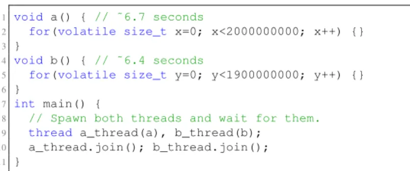
This phenomenon is not limited to I/O operations. Figure 3.1 shows a simple program that illustrates the shortcomings of existing profilers. This program spawns two threads, which invoke
functionsfaandfb respectively. The gprof output for this program is shown in Figure 3.2. Other
profilers may report thatfais on the critical path, or that the main thread spends roughly equal
time waiting forfaandfb [41]. While accurate, all of this information is potentially misleading.
Optimizingfaaway entirely will only speed up the program by 4.5% becausefbbecomes the new
1 void a() { // ˜6.7 seconds
2 for(volatile size_t x=0; x<2000000000; x++) {} 3 }
4 void b() { // ˜6.4 seconds
5 for(volatile size_t y=0; y<1900000000; y++) {} 6 }
7 int main() {
8 // Spawn both threads and wait for them.
9 thread a_thread(a), b_thread(b);
10 a_thread.join(); b_thread.join();
11 }
Figure 3.1: A simple multithreaded program that illustrates the shortcomings of existing profilers.
Optimizingfawill improve performance by no more than 4.5%, while optimizingfb would have no
effect on performance.
% cumulative self self total
time seconds seconds calls Ts/call Ts/call name
55.20 7.20 7.20 1 a()
45.19 13.09 5.89 1 b()
% time self children called name
<spontaneous>
55.0 7.20 0.00 a()
---<spontaneous>
45.0 5.89 0.00 b()
Figure 3.2: A gprof profile for the program in Figure 3.1. This profile shows thatfaandfbcomprise
similar fractions of total runtime. While true, this is misleading: optimizing fa will improve
performance by at most 4.5%, and optimizingfbwould have no effect on performance.
Conventional profilers do not report the potential impact of optimizations; developers are left to make these predictions based on their understanding of the program. While these predictions may be easy for programs as simple as the one in Figure 3.1, accurately predicting the effect of a proposed optimization is nearly impossible for programmers attempting to optimize large applications.
3.2.2 Throughput and Latency
Even if the output of conventional profilers was a useful guide for reducing end-to-end runtimes, profilers would be of limited use for modern software. End-to-end runtime is a proxy for an application’s throughput; the faster it can complete its execution, the greater its throughput. However, the growth in service-oriented software means that latency is an equally important measure of performance in many systems. A service that produces a million responses per second but takes ten minutes between request and response is not useful.
Unfortunately, conventional profilers are not easily adapted to deal with latency. Because they simply report where a program spends its time, they do not distinguish between time spend processing a transaction and other work done by the system. The picture of a program’s execution provided by a conventional profiler includes portions of many transactions, but is often dominated by waiting: even a heavily loaded service often spends much of its time waiting for requests to arrive. To make effective use of a conventional profile, developers of latency-sensitive services must have a near-perfect mental model of their system’s behavior to determine which code is important and which code executes off the critical path for a transaction. While this may be feasible for small programs, developers’ mental models of their systems are often flawed, and these flaws in program understanding can obscure performance bugs [67].
3.3 Building Scalable Software
Service-oriented software poses a special challenge for performance evaluation. These programs are designed to handle heavy load—much more than a single machine can generate—but the per-formance of such a system is highly dependent on the amount and type of load on the system. Like a multi-user system, a software service will process requests from different clients concurrently. However, unlike the multi-user system, these requests are often not independent. An example of one service is the Memcached caching server.
Memcached is a widely-used key-value store typically used as a caching layer in front of a
database. Clients of a memcached server can issuePUTrequests to insert a new value into the cache,
associated with a specified key. AGETrequest searches for a given key and returns the associated
value, if it exists. Because requests from different clients can potentially read and write the same data, access to the set of stored values must be controlled via synchronization. If multiple clients
are issuingGETrequests for a given key, a read-write lock would allow these concurrent requests to
safely execute in parallel. APUTrequest, however, cannot proceed until all readers have released the
lock. If load on the server is sufficiently high, thePUTrequest may never successfully acquire an
exclusive lock on the entry to update the value, a situation known as “writer starvation.”
Resolving this issue could be as straightforward as switching to a different synchronization primitive, such as one that gives writers priority ahead of any later read requests. However, developers are unlikely to fix this issue if they are never able to generate sufficient load on a memcached in
testing to expose the issue. Successfully triggering this issue requires that the test environment is able to generate sufficient load to induce contention, and that the load is representative of real executions.
Unfortunately, for a scalable service, a single machineshould notbe able to generate enough load to
saturate the server; if this were possible, the service would not be scalable.
Even if generating enough load was possible, developers would need enormous traces of all requests to replay in order to generate representative load. These traces are required because issuing
randomPUTandGETrequests would not trigger the scalability issue; it will only occur when many
clients issue concurrentGETrequests for the same key.
One potential workaround for this issue is to embed performance measurement code into deployed services, but this measurement code may have overhead that is unacceptable for deployment. Even if the overhead of performance monitoring is low enough to run in deployment, the results of this performance monitoring will have the same drawbacks as output from conventional profilers; the data tell developers how much time was spent in each part of the program, not which parts of the program to optimize to improve performance in deployment.
CHAPTER 4
STABILIZER: PREDICTABLE AND ANALYZABLE PERFORMANCE
The task of performance evaluation forms a key part of both systems research and the software development process. Researchers working on systems ranging from compiler optimizations and runtime systems to code transformation frameworks and bug detectors must measure their effect, evaluating how much they improve performance or how much overhead they impose [16, 15]. Software developers need to ensure that new or modified code either in fact yields the desired performance improvement, or at least does not cause a performance regression (that is, making the system run slower). For large systems in both the open-source community (e.g., Firefox and Chromium) and in industry, automatic performance regression tests are now a standard part of the build or release process [78, 75].
In both settings, performance evaluation typically proceeds by testing the performance of the actual application in a set of scenarios, or a range of benchmarks, both before and after applying changes or in the absence and presence of a new optimization, runtime system, etc.
In addition to measuringeffect size(here, the magnitude of change in performance), a statistically
sound evaluation must test whether it is possible with a high degree of confidence to reject thenull
hypothesis: that the performance of the new version is indistinguishable from the old. To show that a performance optimization is statistically significant, we need to reject the null hypothesis with high confidence (and show that the direction of improvement is positive). Conversely, we aim to show that it is not possible to reject the null hypothesis when we are testing for a performance regression. Unfortunately, even when using current best practices (large numbers of runs and a quiescent system), the conventional approach is unsound. The problem is due to the interaction between software and modern architectural features, especially caches and branch predictors. These features are sensitive to the addresses of the objects they manage. Because of the significant performance penalties imposed by cache misses or branch mispredictions (e.g., due to aliasing), their reliance on addresses makes software exquisitely sensitive to memory layout. Small changes to code, such as
adding or removing a stack variable, or changing the order of heap allocations, can have a ripple effect that alters the placement of every other function, stack frame, and heap object.
The impact of these layout changes is unpredictable and substantial: Mytkowicz et al. show that just changing the size of environment variables can trigger performance degradation as high as 300% [62]; we find that simply changing the link order of object files can cause performance to decrease by as much as 57%.
Failure to control for layout is a form ofmeasurement bias: a systematic error due to uncontrolled
factors. All executions constitute just one sample from the vast space of possible memory layouts. This limited sampling makes statistical tests inapplicable, since they depend on multiple samples over a space, often with a known distribution. As a result, it is currently not possible to test whether a code modification is the direct cause of any observed performance change, or if it is due to incidental effects like a different code, stack, or heap layout.
4.0.1 Contributions
This chapter presents STABILIZER, a system that enables statistically sound performance analysis
of software on modern architectures. To our knowledge, STABILIZERis the first system of its kind.
STABILIZERforces executions to sample over the space of all memory configurations by
effi-ciently and repeatedly randomizing the placement of code, stack, and heap objects at runtime. We
show analytically and empirically that STABILIZER’s use of randomization makes program execution
independent of the execution environment, and thus eliminates this source of measurement bias. Re-randomization goes one step further: it causes the performance impact of layout effects to follow a Gaussian (normal) distribution, by virtue of the Central Limit Theorem. In many cases, layout
effects dwarf all other sources of execution time variance [62]. As a result, STABILIZERoften leads
to execution times that are normally distributed.
By generating execution times with Gaussian distributions, STABILIZER enables statistically
sound performance analysis via parametric statistical tests like ANOVA [27]. STABILIZER thus
provides a push-button solution that allows developers and researchers to answer the question: does a given change to a program affect its performance, or is this effect indistinguishable from noise?
We demonstrate STABILIZER’s efficiency (< 7%median overhead) and its effectiveness by
SPEC CPU2006 benchmark suite, we find that the-O3compiler switch (which includes argument promotion, dead global elimination, global common subexpression elimination, and scalar
replace-ment of aggregates) does not yield statistically significant improvereplace-ments over-O2. In other words,
the effect of-O3versus-O2is indistinguishable from random noise.
We note in passing that STABILIZER’s low overhead means that it could be used at deployment
time to reduce the risk of performance outliers, although we do not explore that use case here.
Intuitively, STABILIZERmakes it unlikely that object and code layouts will be especially “lucky” or
“unlucky.” By periodically re-randomizing, STABILIZERlimits the contribution of each layout to total
execution time.
4.1 Overview
This section provides an overview of STABILIZER’s operation, and how it provides properties
that enable statistically rigorous performance evaluation.
4.1.1 Comprehensive Layout Randomization
STABILIZERdynamically randomizes program layout to ensure it is independent of changes to
code, compilation, or execution environment. STABILIZERperforms extensive randomization: it
dynamically randomizes the placement of a program’s functions, stack frames, and heap objects. Code is randomized at a per-function granularity, and each function executes on a randomly placed
stack frame. STABILIZER also periodicallyre-randomizesthe placement of functions and stack
frames during execution.
4.1.2 Normally Distributed Execution Time
When a program is run with STABILIZER, the effect of memory layout on performance
fol-lows a normal distribution because of layout re-randomization. Layout effects make a substantial contribution to a program’s execution. In the absence of other large sources of measurement bias, STABILIZERcauses programs to run with normally distribution execution times.
At a high level, STABILIZER’s re-randomization strategy induces normally distributed executions
as follows: Each random layout contributes a small fraction of total execution time. Total execution time, the sum of runtimes with each random layout, is proportional to the mean of sampled layouts.
The Central Limit Theorem states that “the mean of a sufficiently large number of independent random variables . . . will be approximately normally distributed” [27]. With a sufficient number of randomizations (30 is typical), and no other significant sources of measurement bias, execution time
will follow a Gaussian distribution. Section 4.3 provides a more detailed analysis of STABILIZER’s
effect on execution time distributions.
4.1.3 Sound Performance Analysis
Normally distributed execution times allow researchers to evaluate performance usingparametric
hypothesis tests, which provide greaterstatistical powerby leveraging the properties of a known
distribution (typically the normal distribution). Statistical power is the probability of correctly rejecting a false null hypothesis. Parametric tests typically have greater power than non-parametric tests, which make no assumptions about distribution. For our purposes, the null hypothesis is that a change had no impact. Failure to reject the null hypothesis suggests that more samples (benchmarks or runs) may be required to reach confidence, or that the change had no impact. Powerful parametric tests can correctly reject a false null hypothesis—that is, confirm that a change did have an impact—with fewer samples than non-parametric tests.
4.1.4 Evaluating Code Modifications
To test the effectiveness of any change (known in statistical parlance as atreatment), a researcher
or developer runs a program with STABILIZER, both with and without the change. Each run is a
sample from the treatment’spopulation: the theoretical distribution from which samples are drawn.
Given that execution times are drawn from a normally distributed population, we can apply the Student’s t-test [27] to calculate the significance of the treatment.
The null hypothesis for the t-test is that the difference in means of the source distributions is
zero. The t-test’s result (itsp-value) tells us the probability of observing the measured difference
between sample means, assuming both sets of samples come from the same source distribution. If
the p-value is below a thresholdα(typically5%), the null hypothesis is rejected; that is, the two
source distributions have different means. The parameterαis the probability of committing a type-I
It is important to note that the t-test can detectarbitrarily smalldifferences in the means of two
populations (given a sufficient number of samples) regardless of the value ofα. The difference in
means does not need to be5%to reach significance withα= 0.05. Similarly, if STABILIZERadds
4.8%overhead to a program, this does not prevent the t-test from detecting differences in means that
are smaller than4.8%.
4.1.5 Evaluating Compiler and Runtime Optimizations
To evaluate a compiler or runtime system change, we instead use a more general technique: analysis of variance (ANOVA). ANOVA takes as input a set of results for each combination of benchmark and treatment, and partitions the total variance into components: the effect of random variations between runs, differences between benchmarks, and the collective impact of each treatment across all benchmarks [27]. ANOVA is a generalized form of the t-test that is less likely to commit type I errors (rejecting a true null hypothesis) than running many independent t-tests. Section 4.5
presents the use of STABILIZERand ANOVA to evaluate the effectiveness of compiler optimizations
in LLVM.
4.1.6 Evaluating Optimizations Targeting Layout
All of STABILIZER’s randomizations (code, stack, and heap) can be enabled independently. This
independence makes it possible to evaluate optimizations that target memory layout. For example, to
test an optimization for stack layouts, STABILIZERcan be run with only code and heap randomization
enabled. These randomizations ensure that incidental changes, such as code to pad the stack or to allocate large objects on the heap, will not affect the layout of code or heap memory. The developer can then be confident that any observed change in performance is the result of the stack optimization and not its secondary effects on layout.
4.2 Implementation
STABILIZERuses a compiler transformation and runtime library to randomize program layout. STABILIZERperforms its transformations in an optimization pass run by the LLVM compiler [50].
STABILIZER’s compiler transformation inserts the necessary operations to move the stack, redirects heap operations to the randomized heap, and modifies functions to be independently relocatable.