Visualizing Resiliency Of Deep Convolutional Network Interpretations For Aerial Imagery

Rochester Institute of Technology

RIT Scholar Works

Theses

12-2018

Visualizing Resiliency Of Deep Convolutional

Network Interpretations For Aerial Imagery

Bhavan Kumar Vasu

[email protected]

Follow this and additional works at:https://scholarworks.rit.edu/theses

This Thesis is brought to you for free and open access by RIT Scholar Works. It has been accepted for inclusion in Theses by an authorized administrator of RIT Scholar Works. For more information, please [email protected].

Recommended Citation

Visualizing Resiliency Of Deep Convolutional

Network Interpretations For Aerial Imagery

Visualizing Resiliency Of Deep Convolutional

Network Interpretations For Aerial Imagery

Bhavan Kumar Vasu December 2018

A Thesis Submitted in Partial Fulfillment

of the Requirements for the Degree of Master of Science

in

Computer Engineering

Visualizing Resiliency Of Deep Convolutional

Network Interpretations For Aerial Imagery

Bhavan Kumar Vasu

Committee Approval:

Dr. Andreas Savakis Advisor Date

Professor

Dr. Dhireesha Kudithipudi Date

Professor

Dr. Andres Kwasinski Date

Acknowledgments

Firstly, I would like to express my sincere gratitude to my advisor Prof. Andreas

Savakis for the continuous support of my M.S study and related research, for his

patience, motivation, and immense knowledge. His guidance helped me in all the

time of research and writing of this thesis. I could not have imagined having a better

advisor and mentor for my M.S study.

To my life-coach, my father Vasu Narasimhalu: because I owe it all to you. Many

Thanks!

I am grateful to my sister Deepthi and mother Chandrakala , for their moral and

emotional support in life.

A very special gratitude goes out to all down at Kitware Inc. and Air Force

Research Laboratory for helping and providing the funding for my work.

And finally, last but by no means least, also to everyone in the Real time vision

and image processing lab, it was great sharing laboratory with all of you during my

time at Rochester Institute Of Technology.

Abstract

This thesis aims at visualizing deep convolutional neural network interpretations

for aerial imagery and understanding how these interpretations change when network

weights are damaged. We focus our investigation on networks for aerial imagery,

as these may be prone to damages due to harsh operating conditions and are

usu-ally inaccessible for regular maintenance once deployed. We simulate damages by

zeroing network weights at different levels of the network and analyze their effects

on activation maps. Then we re-train the network to observe if it can recover the

lost interpretations. Visualizing changes in the neural network’s interpretation, when

the undamaged weights are retrained, allows us to visually assess the resiliency of a

network.

Our experiments on the AID and the UC Merced Land Use aerial datasets

demon-strate the emergence of object and texture detectors in convolutional networks

com-monly used for classification. We further analyze these interpretations when the

net-work is trained on one dataset and tested on another to demonstrate the robustness

of feature learning across aerial datasets. We also explore the shift in

interpreta-tions when transfer learning is performed from an aerial dataset (AID) to a generic

object dataset (MS-COCO). These results illustrate how transfer learning benefits

the network’s internal representations. Additionally, we explore the effects of various

kinds of pooling operations for class activation map extraction and their resiliency to

coefficient damages.

Finally, we investigate the effects of network retraining by visualizing the change

in the network’s degraded interpretations before and after retraining. Our

visual-ization results offer insights on the resiliency of some of the most commonly used

networks, such as VGG16, ResNet50, and DenseNet121. This type of analysis can

help guide prudent choices when it comes to selecting the network architecture during

Contents

Signature Sheet i

Acknowledgments ii

Dedication iii

Abstract iv

Table of Contents v

List of Figures vii

List of Tables 1

1 Introduction 2

1.1 Motivation . . . 2

1.2 Related Work . . . 3

1.3 Contributions . . . 5

1.4 Organization of The Thesis . . . 6

2 Background work 8 2.1 Datasets . . . 8

2.2 VGG16 . . . 11

2.3 ResNet50 . . . 13

2.4 DenseNet121 . . . 15

2.5 Visualizing Network Interpretations . . . 17

2.6 Class Activation Maps . . . 19

3 Methodology 21 3.1 Aerial-CAM . . . 21

3.2 Class Activation Map Transferability . . . 23

3.3 Evaluation Metrics . . . 24

3.4 Weight Damage . . . 26

3.5 Resilience of network to weight disparities . . . 27

3.6 Retraining . . . 28

CONTENTS

4 Results 31

4.1 Experimental Setup . . . 31

4.2 Aerial-CAM Results . . . 32

4.3 Visualizing CAM Transferability . . . 36

4.4 Comparison of resilience across layers . . . 40

4.5 Comparison of resilience across networks . . . 43

4.6 Effect of Multi-sensor training data on resilience . . . 44

4.7 Retraining Results . . . 45

4.8 Modelling Resiliency of Networks . . . 47

5 Discussion 51 5.1 Future Work . . . 53

Bibliography 54

List of Figures

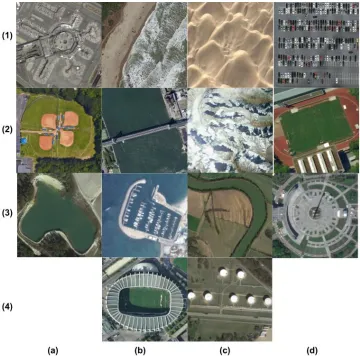
2.1 Sample images from AID dataset for class: (a)(1) Airport, (a)(2)

Base-ball field, (a)(3) Pond, (b)(1) Beach, (b)(2) Bridge, (b)(3) Port, (b)(4) Stadium, (c)(1) Desert, (c)(2) Mountain, (c)(3) River, (c)(4) Storage

Tanks, (d)(1) Parking, (d)(2) Playground, (d)(3) Centre. . . 9

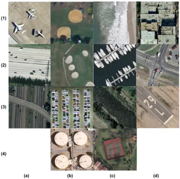
2.2 Sample images from AID dataset for class: (a)(1) Airplane, (a)(2) Free-way, (a)(3)Overpass, (b)(1) Baseball field, (b)(2) Golf course, (b)(3) Parking lot, (b)(4) Storage Tanks, (c)(1) Beach, (c)(2) Harbor, (c)(3) River, (c)(4) Tennis court, (d)(1) Buildings, (d)(2) Intersection, (d)(3) Runway. . . 10

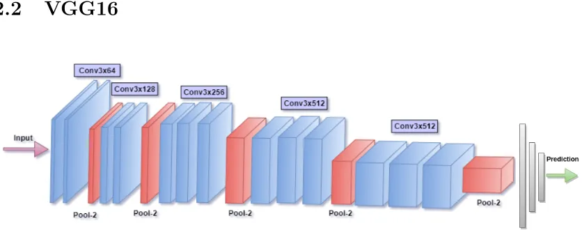
2.3 Graphical representation of the VGG16 architecture . . . 11

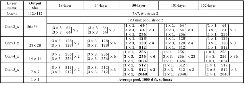
2.4 Difference between a 50 layer plain network (Right) and ResNet50 (Left) 13 2.5 Network architecture variants of ResNet . . . 14

2.6 Structure of each residual blocks in the network . . . 15

2.7 Block diagram for network architecture of DenseNet with three dense blocks . . . 15

2.8 Block diagram of a dense block . . . 16

2.9 Network architeture variants of DenseNet . . . 16

2.10 Visualizing Deep CNN activations in the second and fifth convolution layer of a AlexNet [1] . . . 17

2.11 Visualizing weights after training of an Alexnet from the Initial (Left), Inter-mediate (Center) and Final (Right) convolution layers of an AlexNet [2]. . . 18

2.12 Visualizing activation maps using occlusion [2]. . . 19

2.13 Block diagram for class activation map extraction [3] . . . 20

3.1 Illustration of the Global Average Pooling operation [4] . . . 22

3.2 Block diagram for class activation map extraction [5] . . . 23

3.3 Notation for evaluation metrices p-mAP and cIOU . . . 25

3.4 Illustration of the custom damage layers used to introduce discrepan-cies into the network . . . 27

LIST OF FIGURES

4.1 Examples of CAMs showing the image, its class activation map and

related salient region for the following classes: (a)(1) airport, (a)(2)

storage tanks, (a)(3) desert, (b)(1) baseball field, (b)(2) river, (b)(3)

mountains, (c)(1) beach, (c)(2) center, (c)(3) port, (d)(1) bridge, (d)(2)

stadium and (d)(3) viaduct, using ResNet-50 trained on the AID dataset. 33

4.2 Examples of CAMs showing the image, its class activation map and

related salient region for the following classes: (a)(1) airplane, (a)(2)

intersection, (b)(1) baseball field, (b)(2) overpass, (c)(1) beach, (c)(2)

River, (d)(1) Dense-Residential, (d)(2) Runway and (e)(1) highway,(e)(2)

Storage tanks, (f)(1) Golf course,(f)(2) Tennis court, (g)(1) Harbor and (g)(2) Parking Lot using ResNet-50 trained on the UCM dataset. . . 34

4.3 Comparing of CAMs using LogSumExp (LSE) and Global Average

Pooling (GAP) in a ResNet50 trained on AID: (a) Test Image, (b)

Class Activation Map using LSE, (c) Highest Activation Region (LSE)

(d) Class Activation Map using GAP, (e) Highest Activation Region

(GAP) (1) Beach, (2) Bridge, (3) Storage Tank, (4) Mountain. . . . 35

4.4 CAMs when testing across datasets for known/overlapping classes in

both datasets: (a) baseball field/diamond, (b)(d) beach, (c) river, (e)

ports/harbor and (f) storage tanks. . . 36 4.5 CAMs when testing across datasets for unknown/non-overlapping. Class

activation maps and highest activation regions for classes (a1)(b1) golf

course and (c1)(d1) intersection when trained on AID and testing on

UCM. Column (2) is for classes (a2)(b2) bridge and (c2)(d2) mountains

when training on UCM and testing on AID. . . 37

4.6 Class activation maps for 14 classes in the MS-COCO dataset when

training on AID and processing MS-COCO images before transfer

learning (blocks 1 and 2) and after transfer learning (blocks 3 and 4).

Examples shown from classes (a)(1) tooth brush, (b)(1) pizza, (c)(1) person and giraffe, (d)(1) person skiing, (e)(1) food on table, (f)(1)

per-son playing baseball, (g)(1) train, (a)(2) perper-son furniture, (b)(2) food,

(c)(2) clock and person, (d)(2) clock, (e)(2) giraffe, (f)(2) suitcase and

LIST OF FIGURES

4.7 Class activation maps for 14 classes in the MS-COCO dataset when

training on AID and processing MS-COCO images after transfer

learn-ing (blocks 1 and 2) and after transfer learnlearn-ing (blocks 3 and

4).Ex-amples shown from classes (a)(1) tooth brush, (b)(1) pizza, (c)(1)

son and giraffe, (d)(1) person skiing, (e)(1) food on table, (f)(1)

per-son playing baseball, (g)(1) train, (a)(2) perper-son furniture, (b)(2) food,

(c)(2) clock and person, (d)(2) clock, (e)(2) giraffe, (f)(2) suitcase and

book, (g)(2) food. . . 39

4.8 VGG16 at damage levels 25%,50% and 75% . . . 40

4.9 ResNet50 at damage levels 25%,50% and 75% . . . 41

4.10 DenseNet121 at damage levels 25%,50% and 75% . . . 42

4.11 Comparing resilience across VGG16, DenseNet121 and ResNet50 . . . 43

4.12 Comparing resilience of ResNet50 trained on AID and UCM dataset . 45 4.13 Results for VGG16 before and after retraining from damages . . . 46

4.14 Results for ResNet50 before and after retraining from damages . . . . 47

List of Tables

2.1 Table showing the number of images present in each of the 14 AID

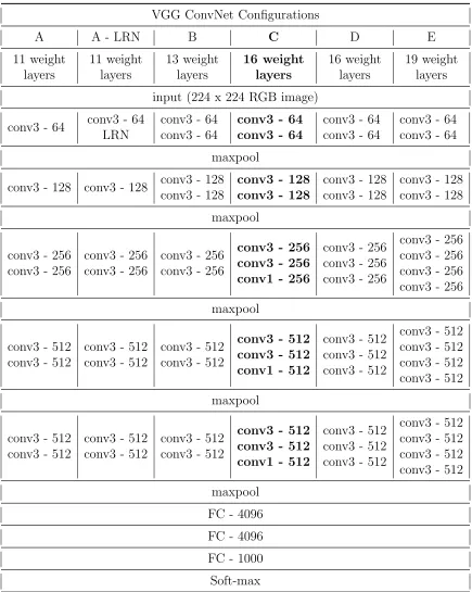
dataset classes . . . 9 2.2 Network architecture variants of VGG. . . 12

4.1 Table showing the training and testing accuracy of VGG16, ResNet50

Chapter 1

Introduction

1.1

Motivation

The ultimate goal of AI is to emulate the capabilities of the brain. Our efforts to

surmount this daunting task considering that we still struggle to understand our own

cognitive mechanism on both scientific and spiritual level. While the worlds most

sophisticated supercomputer can require the energy equal to about 750,000 light bulbs

while our brain can do all of that work on roughly 20 watts of energy, that’s about

what one light bulb uses. Recent cognitive studies on some patients diagnosed with

brain hemorrhage show that the brain can undergo a re-organization phase, where

the functions of the damaged neurons were taken up by the undamaged neurons,

over time. This thesis tries to explore such resiliency capabilities present in some

of the most commonly used convolutional neural networks. A convolutional neural

network is deployed by exporting the graph and weights of the network. The graph

expresses the structure or connectivity and the weights decide the strength of the

connection. Damages to the network weights could make the network useless once

deployed. Studying the effects of such weight damages on network interpretations

plays an important role in finding solutions enabling neural networks to pass on their

features onto the undamaged weights with minimal re-training.

CHAPTER 1. INTRODUCTION

classification [6], [7], [8], the application of deep learning algorithms in the field of

remote sensing has potential to widen the amount of information that can be

ex-tracted from satellite imagery [9], [10]. Using deep CNN architectures can benefit

a variety of applications, such as disaster management, demographic estimation,

ge-ologic research, security, environmental conservation etc. Visualizing CNN internal

representations is a way to better understand the way deep networks interpret images

[2], [11], [3]. However, research in network visualization has been limited to Imagenet

types of datasets [12] without considering aerial imagery, which is growing in volume

and significance. The acquisition and accessibility of aerial and remote sensing images

are steadily increasing due to the proliferation of Unmanned Aerial Vehicles (UAVs)

and commercial satellite systems from companies such as Planet and Digital Globe.

When deep networks are deployed in orbiting satellites or high altitudes platforms,

they may experience damage or failures. Failures can inevitably occur in the network

and it is important to understand their implications. This thesis investigates the

impact of such damages to the inner workings of networks trained on aerial imagery

by visualizing class activation maps and how they change. This method of evaluating

resiliency of networks can be extended to other deep networks expected to operate in

challenging environments. The resiliency of the network connections can be viewed

as its ability to maintain its initial interpretation even after damages or undesirable

change to its connections have occurred. This thesis proposes to map these CNN

inner representations of aerial images for damages that occur at different stages of

the network.

1.2

Related Work

Visualizing how the deep CNN interprets an image and visualizing spatial information

learned by filters at different levels of the network is an important area of research.

tech-CHAPTER 1. INTRODUCTION

niques for the understanding of a CNN. They presented three techniques to make

sense of what CNNs are learning by visualizing activation, visualizing weights and

understanding CNNs using the occlusion experiment. All three methods are described

in Chapter 2. But these methods resulted in low resolution or noisy representations

of the activated features. Cook [13] introduced Global Average Pooling (GAP) for

neural networks, enabling us to compute a single linear vector for all the the feature

maps from the final layer. When used with neural networks, the GAP layer can be

used to get class activation maps as demonstrated in [3]. It uses a weighted sum of

the features maps responsible for classification of the image to class c. The work in

[14] aims to visualize what the network learns using a DeconvNet [15] to get pixel

level predictions for different textures. Alternatively, [3] attempted to visualize the

network representations using linear classifier probes instead of a DeconvNet. Bau

and Zhou adopted a more flexible approach to classifying a broader set of features

by shedding light on how a CNN has remarkable localization abilities despite

be-ing trained on image-level labels trained on ImageNet [12] and other datasets like

Places-365 [14].

The work in [16] proposed a method to train a single CNN on aerial imagery

for efficiently classifies multiple objects using feature maps from the last layer, but

limited its analysis to just roads and buildings. The work in [17] partially addresses

the emergence of object detectors in a network trained for aerial image captioning

using several CNN and Long-Short Term Memory networks (LSTMs) trained on the

UC Merced dataset. This work motivated the application of the network dissection

techniques described in [3], [18], [3] to aerial imagery.

The effect of modifications of network weights on performance was analyzed in

[19], [20], where the weights in the network are altered by introducing a unique stress

function and reduction techniques are used for different kinds of weight drops. In [19]

CHAPTER 1. INTRODUCTION

weights. [21] was the first attempt towards exploring new propagation methods for

retraining networks more resiliently. More recently, the work in [22] established a

framework for estimating resiliency of DCNN’s by understanding the relationship

between fault rate and model accuracy.

Our work differs, as we visualize weight damages from the network’s perspective

using class activation mapping. We draw a clear picture of the resiliency of a network

after checking the class activation maps. Class activation mapping essentially gives us

a picture of the spatial information in the test image that a deep CNN considers most

important as it remembers from its training phase. Visualizing the effect of damages

to these networks allows us to visualize the variability of the network interpretations

as the network weights degrade. Finally, we use retraining propagation techniques

such as Stochastic Gradient Descent (SGD) to efficiently help the network heal by

using a small set of training images trying to recover the lost interpretation hence

quantifying resiliency of several commonly used deep neural network. After gaining

a clear insight into the deep CNN interpretations for aerial imagery, we use these

interpretations as a metric to visually assess the amount of information lost due to

damaged weights in the network.

1.3

Contributions

The main contributions of this thesis are:

• Visualize CNN internal interpretations of remote sensing imagery through class

activation maps and demonstrate the network’s ability to localize its

represen-tations using GAP.

• Quantify and map the resiliency of network interpretations in a CNN to the

cor-responding amount of network weight disparities caused due to damaged/corrupt

CHAPTER 1. INTRODUCTION

• Compare resiliency across the three most widely used deep CNN architectures

in the field of classification.

• Visualize the effect of retraining the network, which helps the healthy weights

to recover the networks lost interpretation after substantial damage.

• Show that CNN representations are transferable from one dataset to other by

evaluating their transfer-ability between dataset with similar classes and data

sets with unknown classes that it has not seen during training.

• Build a statistical model of network interpretations from a damaged and

re-trained network.

• Publications:

– Vasu, Bhavan, Faiz Ur Rahman, and Andreas Savakis. “Aerial-CAM:

Salient Structures and Textures in Network Class Activation Maps of

Aerial Imagery.” 2018 IEEE 13th Image, Video, and Multidimensional

Signal Processing Workshop (IVMSP), 2018.

– Rahman, Faiz Ur, Bhavan Vasu, and Andreas Savakis. “Resilience and

Self-Healing of Deep Convolutional Object Detectors.” 2018 25th IEEE

International Conference on Image Processing (ICIP), 2018.

1.4

Organization of The Thesis

The thesis is organized in five chapters. Brief information about each chapter is

mentioned below:

• Chapter 1. Introduction: explains the motivation behind the work that has been

performed toward completing the thesis, literature review about the proposed

CHAPTER 1. INTRODUCTION

• Chapter 2. Background Work: Overviews previous methods used to visualize

network interpretations and a brief overview of the different architectural styles

and their examples. Later part of this chapter describes the datasets that were

used in this thesis in details.

• Chapter 3. Methodology: describes the methodology to visualize activation

maps in aerial imagery and simulate damages to network weights. Followed

by a detailed explanation of the evaluation metrics used to estimate resiliency.

Re-training protocols followed to heal damaged networks and finally more on

how we plan to model resiliency of network.

• Chapter 4. Results: compares results for each of the methodologies described in

Chapter 3 on AID, UCM, and MS-COCO. This includes comparisons between

the networks and layers within networks.

• Chapter 5. Discussion: mentions a brief summary of the thesis and the obtained

Chapter 2

Background work

This chapter starts by describing the dataset used for our analysis. Section 2.2 to 2.4

gives a brief introduction to the three models VGG16, ResNet50 and DenseNet121,

and their architectural style. Understanding their architecture acts as a base to

interpret their behavior when network weights are damaged.

2.1

Datasets

The networks under investigation were trained on aerial images using a subset of the

publicly available AID Dataset [9] and the UC Merced Land Use Dataset (UCM).

The considered AID subset contains images with a single ground truth for aerial

scene recognition problem for 14 classes such as airports, storage tanks, mountains,

ports, rivers, viaducts, bridges, desert, beaches, baseball field, center, railway stations,

resorts, and stadiums. The AID dataset contains images of size 600×600 and multiple

ground sample distances (GSDs).

The UC Merced (UCM) images are of size 256×256 from 14 classes: airplane,

beach, storage tanks, runway, parking lot, river, overpass, intersection, golf course,

harbor, freeway, dense residential, buildings, and tennis courts, captured at 1-foot

resolution. The UCM contains 100 images for every class in the dataset. The AID

dataset was chosen as the primary dataset for our analysis because of its high

CHAPTER 2. BACKGROUND WORK

Figure 2.1: Sample images from AID dataset for class: (a)(1) Airport, (a)(2) Baseball

field, (a)(3) Pond, (b)(1) Beach, (b)(2) Bridge, (b)(3) Port, (b)(4) Stadium, (c)(1) Desert, (c)(2) Mountain, (c)(3) River, (c)(4) Storage Tanks, (d)(1) Parking, (d)(2) Playground, (d)(3) Centre.

Table 2.1: Table showing the number of images present in each of the 14 AID dataset

classes

AID

Class # of images Class # of images

airport 360 storage tanks 360 baseball field 220 viaduct 420

bridge 360 river 410

center 260 port 380

beach 400 square 330

desert 300 stadium 290

CHAPTER 2. BACKGROUND WORK

Figure 2.2: Sample images from AID dataset for class: (a)(1) Airplane, (a)(2) Freeway,

(a)(3)Overpass, (b)(1) Baseball field, (b)(2) Golf course, (b)(3) Parking lot, (b)(4) Storage Tanks, (c)(1) Beach, (c)(2) Harbor, (c)(3) River, (c)(4) Tennis court, (d)(1) Buildings, (d)(2) Intersection, (d)(3) Runway.

unlike single source images in the UC Merced dataset. We also use the MS-COCO

dataset [23] for visualizing resulting Class Activations Maps after performing transfer

learning. The three networks namely: VGG16, ResNet50 and DenseNet achieved

different testing accuracies on the two datasets solely depending on their architecture.

The above three networks were chosen in order to note the difference in resiliency

between VGG and residual type architectures. The comparison between ResNet

and DenseNet further allow us to see the effect of addition and concatenation skip

connections on network performance. The next sections of this chapter are a brief

CHAPTER 2. BACKGROUND WORK

2.2

VGG16

Figure 2.3: Graphical representation of the VGG16 architecture

The VGG16 [6] is a neural network that can be expressed as a stack of

convo-lutional layers that contain filters of kernel size 3 in order to maintain the spatial

integrity of features calculated from their input. Care is taken in maintaining the

spatial resolution during convolution by having a spatial padding of 1 pixel for every

convolutional layer with a kernel size 3. Groups of convolutional layers with a fixed

number of filters make up a convolutional block. These convolutional blocks are

fol-lowed by a 2×2 spatial pooling with a stride of 2. The output from this stack of

convolution blocks is fed into a fully connected network with 3 fully connected

con-volutional layers with the first two layers having 4096 filters and the final layer made

up of 1000 filters which is nothing but the number of classes to classify in ImageNet

as shown in Table 4.1. The output from each hidden layer in the network is passed

through a non-linearity in the form of a Rectified Linear Units (ReLU). Figure 2.3

shows an illustration of a 16 layer VGG network with input size 224×224×3.

Fea-tures from the final convolution layer was passed into the fully connected network to

give us a prediction. During the test phase, all the weights are frozen and the input

is passed through the series of hidden layers in a feed-forward manner to classify the

CHAPTER 2. BACKGROUND WORK

VGG ConvNet Configurations

A A - LRN B C D E

11 weight layers 11 weight layers 13 weight layers 16 weight layers 16 weight layers 19 weight layers

input (224 x 224 RGB image)

conv3 - 64 conv3 - 64 LRN

conv3 - 64 conv3 - 64

conv3 - 64 conv3 - 64

conv3 - 64 conv3 - 64

conv3 - 64 conv3 - 64

maxpool

conv3 - 128 conv3 - 128 conv3 - 128 conv3 - 128

conv3 - 128 conv3 - 128

conv3 - 128 conv3 - 128

conv3 - 128 conv3 - 128

maxpool

conv3 - 256 conv3 - 256

conv3 - 256 conv3 - 256

conv3 - 256 conv3 - 256

conv3 - 256 conv3 - 256 conv1 - 256

conv3 - 256 conv3 - 256 conv3 - 256

conv3 - 256 conv3 - 256 conv3 - 256 conv3 - 256

maxpool

conv3 - 512 conv3 - 512

conv3 - 512 conv3 - 512

conv3 - 512 conv3 - 512

conv3 - 512 conv3 - 512 conv1 - 512

conv3 - 512 conv3 - 512 conv3 - 512

conv3 - 512 conv3 - 512 conv3 - 512 conv3 - 512

maxpool

conv3 - 512 conv3 - 512

conv3 - 512 conv3 - 512

conv3 - 512 conv3 - 512

conv3 - 512 conv3 - 512 conv1 - 512

conv3 - 512 conv3 - 512 conv3 - 512

conv3 - 512 conv3 - 512 conv3 - 512 conv3 - 512

maxpool

FC - 4096

FC - 4096

FC - 1000

Soft-max

CHAPTER 2. BACKGROUND WORK

2.3

ResNet50

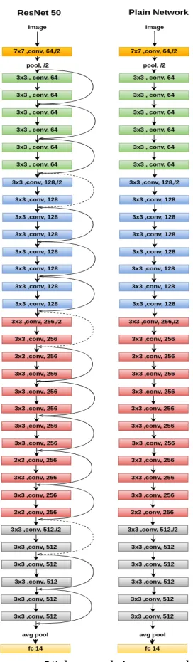
Figure 2.4: Difference between a 50 layer plain network (Right) and ResNet50 (Left)

With the huge success of VGG type architectures in image classification, the race

to go deeper had begun. But going deeper gave rise to new problems with vanishing

gradients and global optimal convergence. Even though going deeper decreased the

classification error on ImageNet, as networks got deeper, training them to reach a

CHAPTER 2. BACKGROUND WORK

Figure 2.5: Network architecture variants of ResNet

the gradients becoming insignificant as they propagate deep into the network, forcing

the initial layer to learn redundant features. The classification error also increased

after plateauing at the later stages of training. The solution to this problem came in

the form of residual connections in ResNet type architectures that bypass blocks of

convolutional layers and re-enforce the input of nth layer to some (n+x) th layer,

solving the vanishing gradients problem. In residual learning, instead of trying to

learn class specific features, the network tries to learn some residual that is simply a

subtraction of features learned from the input of that layer. By stacking these layers,

the gradient could theoretically skip over all the intermediate layers and reach the

bottom without being diminished. We use ResNet50 [7] architecture for our analysis.

The ResNet50 is a 50 layer Residual Network as shown in figure 2.2. The other

variants of ResNet type architecture with more than 50 layers include ResNet101 and

ResNet152 also.

The ResNet50 is a version of residual networks with 3 convolution layer with two

1×1 kernels and one 3×3 kernels as shown in the highlighted column of Figure 2.6.

Figure 2.4 shows the difference between a plain VGG style 50 layer network (Right)

and a ResNet50 (Left) architecture with skip connections. These skip connections

helped gradients reach deeper layers, hence allowing network designers to go hundreds

CHAPTER 2. BACKGROUND WORK

Figure 2.6: Structure of each residual blocks in the network

is prevented by the skip connection addition of information entering the block and

leaving the block.

2.4

DenseNet121

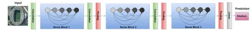
Figure 2.7: Block diagram for network architecture of DenseNet with three dense blocks

The Densenet architecture [8] is an extension of the ResNet architecture. The

ResNet architecture has a fundamental identity block that performs addition between

input from a previous layer and a future layer, forcing the network to learn residuals.

Recent studies on ResNets show that many layers contribute very little or redundant

features and can, in fact, be randomly dropped during training. In contrast, the

DenseNet architecture in Figure 2.7 concatenates outputs from the previous layers

instead of adding them given by

CHAPTER 2. BACKGROUND WORK

Where x, x−1...x−n are the output of previous layers.

For each layer, the feature-maps of all preceding layers are used as inputs, and

the current layer’s feature-maps are used as inputs into all subsequent layers given

by Equation (2.1). Concatenating feature maps learned by different layers increases

variation in the input of subsequent layers and improves efficiency. This dense

con-nectivity pattern not only solved the vanishing gradient problem but also required

fewer parameters than traditional convolutional networks due to feature reuse and

stronger feature propagation.

Figure 2.8: Block diagram of a dense block

Figure 2.9: Network architeture variants of DenseNet

CHAPTER 2. BACKGROUND WORK

information and gradients throughout the network, which makes them easy to train.

In a feed forward setting the final layers benefit from the low-level features along

with high level features from the later parts of the network. This enables the network

to learn complex scenes as it can look at both edges and high level features for its

classification. Each layer in a DenseNet has direct access to the gradients from the

loss function and the original input signal, leading to an implicit deep supervision

shown in Figure 2.8. We use the DenseNet-121 for our analysis. Some variants of the

DenseNet style architectures are DenseNet-161, DenseNet-169, DenseNet-201 shown

in Figure 2.9

2.5

Visualizing Network Interpretations

Early attempts to visualize network interpretation were carried out by visualizing the

activation at each layer in the forward pass [2]. For networks using ReLU activation,

studies have shown that activations start out blobby and dense. The activations get

more sparse and localized as training progresses. This method gives us all activations

both important and dead ones as shown in Figure 2.10 [2].

Figure 2.10: Visualizing Deep CNN activations in the second and fifth convolution layer

of a AlexNet [1]

CHAPTER 2. BACKGROUND WORK

the network learns during training. For well-trained networks, the trainable weights

tend to be more smooth and noiseless to visualize compared to activations. Visualizing

the network filter weights requires a DeconvNet for switched pooling as described by

Matthew in [2]. We obtain a visual interpretation of the network weights by using

transposed versions of the filter on the recitifed maps. The switch setting in the

max-pool present on the DeconvNet is identical to the max-pooling setting in the convnet to

make sure the projection is consistent. Weights from the initial layers are generally

a good representation of the input data as they look at the input image directly.

Figure 2.11: Visualizing weights after training of an Alexnet from the Initial (Left), Inter-mediate (Center) and Final (Right) convolution layers of an AlexNet [2].

We can observe from Figure 2.11 that the network over time builds a dictionary of

low-frequency color filters and high-frequency gray-scale features in the initial layers.

This is a consequence of the network architecture. Since the model is trained

dis-criminatively, they implicitly show which parts of the input image are discriminative

across different classes in the input dataset. We observe that the initial layers learn

low-level features and the abstraction of features increases as we move from initial

to final layers. To visualize a given convnet’s activation, we set all other activations

in the layer to zero and pass the feature maps as input to the attached deconvnet

layer. Then we successively unpool, rectify and filter to visualize filters in the layer

beneath. After visualizing the kind of features neural networks look at, in both high

CHAPTER 2. BACKGROUND WORK

Figure 2.12: Visualizing activation maps using occlusion [2].

part of the image made the network classify a particular test image as belonging to

class c. This also acts as a sanity check for making sure if the model is truly

identi-fying the location of the object in the image, or just using the surrounding context

to classify it. Occlusion sensitivity study helps us answer this question by giving us

a heatmap of the test image signifying the semantic structures of importance. This

activation map is achieved by systematically occluding different portions of the input

image with a grey square. An area of importance can be identified when occlusion

causes the class probability to drop by a huge margin. This process is continued for

all possible occlusions in the test image, resulting low-dimensional heatmaps as shown

in Figure 2.12. The blue regions signify pixels that lead to a low probability when

occluded, in turn signifying high importance.

2.6

Class Activation Maps

The network largely consists of convolutional layers, and a global average pooling

layer just before the final softmax layer. Given this basic architecture, we can extract

CHAPTER 2. BACKGROUND WORK

back the weights of the output layer on to the convolutional feature maps, a technique

called as class activation mapping.

Figure 2.13: Block diagram for class activation map extraction [3]

A Class Activation Map (CAM) [3] is the localized region of the image that most

influences the decision of the network for a class of images. The dimensionality

re-duction layers let us compute a weighted sum of the feature maps from the last

convolutional layer providing the class activation map for the predicted class.

Acti-vated regions are decided by the top contributing weights for the network to make a

decision. For a given feature map, let fk_{(x, y) represent the activation of unit k in}

the last convolutional layer at the x, y location in the test image. The class specific

weights wk

c after the GAP layer is multiplied with k feature maps

P

x,yf

k_{(x, y) that}

signifies the importance of each of the k activations from the final convolution layer.

The CAM, F(x, y) for an aerial scene belonging to class c is given by Equation (2.2).

F(x, y) = X k

w_ckfk(x, y) (2.2)

Since we already know each unit activates for a particular visual pattern in the input

image. A class activation map can be defined as a simple weighted linear sum of the

Chapter 3

Methodology

3.1

Aerial-CAM

We explore the visualization of Class Activation Maps (CAMs) in aerial images [5]

with the objective of gaining insights on how CNN’s interpret these images for

clas-sification. Class activation maps extracted using the procedure discussed in Section

2.6 are used for all further experiments. Class activation map extraction can be

per-formed on any network if it contains a Global Average Pooling layer as its penultimate

layer. The final layer can be a simple softmax layer used for classification. The Global

Average Pooling was born as a result of researcher’s attempt to prevent over-fitting

caused due to the fully connected layers used before the softmax layer. The softmax

layer takes in K dimension vector and the predicts probability P for the jth _class

given a sample vector n and a weighting vectorp, P is given by

P(y=j |n) = e nT_p

j

PK k=1en

T_p

k

(3.1)

This over-fitting affects the generalization ability of the network. Whereas Global

Average Pooling (GAP) helps in enforcing correspondences between feature maps

and categories enabling us to interpret feature maps as confidence maps. Since the

CHAPTER 3. METHODOLOGY

Figure 3.1: Illustration of the Global Average Pooling operation [4]

over-fitting.

G(k) = _W1_∗H P

x,yk(x, y) k∈W ×H×K (3.2)

where W and H are the width and height of the feature map k ∈K features maps.

The output of the GAP layer G at position k is given by the average of each feature

map resulting in 1×Kdimensional vector. The global average pooling can be replaced

by other dimensionality reduction layers such as LogSumExp (LSE) layer given by

Equation (3.4) to generate class activation maps .

LSE(k1, . . . , kn) =x∗+ log (exp(x1−x∗) +· · ·+ exp(xn−x∗)) (3.3)

where,

x∗ = max{x1, . . . , xn}x∗ = max{x1, . . . , xn} (3.4)

The LSE flattens each feature map to obtain vector x that can be used to calculate

the LSE of the features from the final layer of our network using Equation (3.3).

This is due to the fact that LSE also results in a single dimension vector of size

equal to k units in the previous layer, where thekthvalue after reduction is signifying

the importance of the kth unit as shown in Fig 3.1. As illustrated in Fig. 3.2, we

experiment with the Global Average Pooling and LogSumExp layer to demonstrate

CHAPTER 3. METHODOLOGY

Figure 3.2: Block diagram for class activation map extraction [5]

Since the CAMs extracted from GAP and LSE were nearly identical, we only consider

the interpretations extracted using GAP for most experiments as it is native to several

network architectures. We threshold and up-sample these class activation maps to

obtain a mask that can be placed over our input image for better localization of the

highest activating region.

3.2

Class Activation Map Transferability

After procuring knowledge regarding the kind of structures that make a deep CNN

classify a particular aerial scene, this thesis investigates how these interpretations

are affected by some well-known techniques like transfer learning. Transfer learning

is a machine learning method where a model developed for a task is reused as the

starting point for a model on a second task. We study the effect of transfer learning

on class activation maps. Performing transfer learning between two similar tasks and

transfer learning on two completely different tasks gives us insight into the CAM’s

transferability from one dataset to other. The experiment to determine CAM

trans-ferability uses three data sets namely, AID, UCM, and MS-COCO. The AID and

CHAPTER 3. METHODOLOGY

aerial scene classification while the MS-COCO constitutes a dataset for a completely

different task like eye-level image classification.

We test each one of our networks for CAM transferability by formulating the

following three experiments

• Compare Class activation maps for common classes between AID and UCM.

• Compare Class activation maps for classes not shared between AID and UCM.

• Visualize Class activation maps for AID/UCM using a network trained on

MS-COCO and vice versa.

Since the image classes from MS-COCO dataset are completely different compared

to classes from both the AID/UCM, comparing their interpretation should give us an

idea of their adaptability. And comparing CAM between AID and UCM should tell

about their transferability within the same problem domain.

3.3

Evaluation Metrics

We evaluate the quality of the localization after damage using permuted mean average

precision (p-mAP) [24] and cIOU [24]. For each image, the extracted class activation

map after damage is an unnormalized probability mappthat is binarized by selecting

the optimal threshold per image (0.8 times the peak value in p). The resulting image

after multiplying with our binary mask is the activation region. Similarly we compute

the binarized and post-threshold mask m when the network is unharmed. The two

activated regions before and after damage serve as our m and p. The symmetrized

average precision s(m, p) between m and p accounts for the non-activated regions

that might result in a higher accuracy. The symmetrized average precision is given

by Equation (3.6).

s(m, p) = 1

CHAPTER 3. METHODOLOGY

Figure 3.3: Notation for evaluation metrices p-mAP and cIOU

and p-mAP becomes

p-mAP =max(s(m, p), s(1−m,1−p)) (3.6)

Fig 3.3 explains the area of pixels considered astp,fp,tn, and fn when comparing

the two highest activating regions. Even though the p-mAP value does not always

capture the interpretation loss perfectly, it follows a trend that is evident when plotted

at different damage levels D%. Therefore, we also evaluate the model with cIOU, the

mean IOU of two regions of activation, because we only have two classes, that is

the activation below the threshold and above the threshold. This lets us implement

everything in terms of tp, tn,fp, fn by Equation (3.7).

cIOU = (tp/(tp+fp+fn) +tn/(tn+fp+fn))/2. (3.7)

wheretp represents the image pixels present in the union of the regions of the images

that were activated before damage and after damage; fp represents the image pixels

not present in activation before damage but were seen an important part of the image

com-CHAPTER 3. METHODOLOGY

parison before damage and after retraining. Section 3.4 goes over our methodology

to introduce weight damages in the network.

3.4

Weight Damage

Once we understand what the network interpretations for a particular class of

im-ages look like and how they adapt over different datasets, it is time to visualize the

resiliency of these interpretations. Resiliency is the capacity to recover quickly from

damage. We compare resiliency of features extracted in different networks and their

dependence on weights from different layers of the same network. Weight damage

could occur when the network is deployed in a remote location. Studying the

be-havior of activation maps after damages enables us to map the network bebe-havior

during these damage phases so we can have an estimate of its performance without

directly accessing the network. In this work, the damages to the network are spread

randomly among weights at the node of analysis. Following this approach, we

intro-duce weight damage at four levels D1, D2, D3 and D4, for all our three networks

VGG16, ResNet50, and DenseNet121. These selected nodes are all present in the

first convolution layer of each network block. We select nodes starting from the first

layer in case the network has more than 4 blocks in its architecture. For example in

VGG16 we damage weights from the first convolution layer in the first four blocks

and in ResNet50 we do the same every time the number of filters doubles for all 3×3

kernels. If a layer contains N trainable weights, we drop D% of N weights.

Dropping network weights is forcing the selected weights to zero, simulating the

stuck at zero damage. A network weight that is zero signifies a dead node in a graph

as it has no connection leaving the node. We perform this kind of dropping at the

starting of a block. The amount of damage D% is swept from 5% to 95% of the total

number of weights in a given layer across all filters between the convolutional layersk

CHAPTER 3. METHODOLOGY

Figure 3.4: Illustration of the custom damage layers used to introduce discrepancies into the network

nodes is carried out until we get activation maps from the network for all possible

D1, D2, D3 and D4 combinations. The skip connections in both the ResNet50 and

DenseNet121 are not altered.

Once damaged, the network weights are permanently disabled in the test and

re-train phase. Therefore, only the undamaged weights are updated during rere-training,

while gradient flow to the damaged weights is disabled. The locations of weight

dis-ruptions were chosen with the objective to push the networks to their limits. This

approach regulates the amount of information dropped in each stage for all our

ex-periment.

3.5

Resilience of network to weight disparities

After introducing faults in the network architecture, the proposed method tries to

measure their effect on network interpretations.

Damages simulated to the network using the methodology described in Section

3.5 causes degradation of network interpretation, but mapping this degradation in

interpretation allows us to appreciate the resilience of some commonly used networks

CHAPTER 3. METHODOLOGY

Figure 3.5: Block diagram for the methodology to determine visual resiliency

manner and calculate the corresponding cIOU score between the interpretation

ex-tracted from an undamaged network and the degraded interpretation after damage as

shown in Fig 3.5. We continue this process until we have a cIOUdrop associated with

every possible value of D1, D2, D3 and D4 between 5% to 95%. After our analysis

of the damaged network, we attempt the retrain it and compare the cIOU of the

retrained network against the undamaged network to make sense of the effectiveness

of retraining.

3.6

Retraining

Retraining can either help in re-enforcing already existing network interpretation or

adapt to new interpretations with the limited number of weights remaining in the

network after damages to its weights. We believe this rise in new interpretation is

due to the network trying to change its interpretation with respect to the available

number of weights at its disposal. But the new interpretation cannot be scored higher

as it is not the best possible interpretation the network can learn. The retraining is

CHAPTER 3. METHODOLOGY

learning. This is achieved by forcing the damaged weight and gradient value to zero

at every iteration of the network. Retraining a damaged network does not require a

large amount of data, but having a smaller dataset with a good range of examples

belonging to the class is more important.

We put together a smaller subset of the original training data that was used to

train the network. In our experiments, we choose 25% of the original samples in

the training dataset and use the same testing dataset used during training. We use a

standard Stochastic Gradient Descent (SGD) to retrain the network for only 4 epochs.

We extract the CAM of the retrained network one last time in order to compute the

cIOU and p-mAP of the network interpretation over the same test samples.

Com-paring the cIOUdrop after damage and cIOURetrain after retraining should let us judge

the resiliency of different networks and layers in those networks. Since the number of

samples in the UCM dataset were limited, we use the whole training dataset to

re-train the network. This ensured both the rere-training sets for our analysis on AID and

UCM were of comparable size. Since, we have an idea of the network’s performance

before damage, after damage and after retraining, we attempt to model the network

resiliency in the next section.

3.7

Modelling Resiliency

Modeling resiliency is our final experiment that leverages all the knowledge we gained

so far regarding network resiliency and salience of network interpretation by treating

this as a multi-linear regression problem. The compiled data on the amount of damage

at different nodes vs cIOUdropor cIOURetraincan be used to model and predict network

interpretation quality for any given damage level. We perform multi-linear regression

on the damage levels at each node of the network for the different style of architectures

and attempt to model their behavior. Modeling it as a multiple linear regression

CHAPTER 3. METHODOLOGY

and network interpretation. It should also let us isolate the influence of two closely

related damage levels in influencing the cIOU score.

We present different linear equations that relate the amount of damages at each

stage of the network to the final cIOU score. The R2 _{of the fitted models were closely}

monitored to oversee the goodness of fit. We also make sure our residual plot carries

randomly distributed residual data points, indicative of no meaningful structure left

in the data. Equation (3.8) shows a form of the desired data model.

cIOU =b1∗D1 +b2∗D2 +b3∗D3 +b4∗D4 (3.8)

Where coefficientb1,b2,b3 and b4 signify the importance of the damage in nodeD1,

D2,D3 and D4 respectively for calculating cIOU. This cIOU can either be cIOUdrop

or cIOURetrain. This should let us make an informed choice when trying to pick

Chapter 4

Results

4.1

Experimental Setup

We experiment with the layer and amount of damage in different networks. Four

layer locations were chosen for the VGG16 network, one at the beginning of each

convolution block. Similarly, we choose four locations for our experiments with the

ResNet50 and DenseNet121 architecture. The amount of damage at these layers

is independently varied from 5% to 95% in increments of 5% and respective class

activation maps are extracted after damage. The class activation map is observed to

be degraded compared to the original activation map. This extracted activation is

compared to the activation acquired from an unharmed network using a permuted

mean average precision (p-mAP) [24] and cIOU to quantify the resiliency of the

networks.

The ResNet-50 is a narrow 50 layer residual network that was proposed in [7] and

Densenet 121 proposed in [8] was inspired from ResNet but had substantially fewer

trainable parameters whereas VGG16 is a densely connected feedforward network. All

three architectures were trained separately on the AID and UCM datasets to classify

14 classes. We obtained a training accuracy of 96.3% and 94.2% with a validation

accuracy of 92.4% and 91.7% on the AID and UCM dataset respectively using the

CHAPTER 4. RESULTS AID UCM Training Accuracy (%) Test Accuracy (%) Training Accuracy (%) Test Accuracy (%)

VGG16 94.3 94.1 92.2 91.8

ResNet50 96.3 92.4 94.2 91.7

DenseNet121 98.74 96.8 95.6 93.87

Table 4.1: Table showing the training and testing accuracy of VGG16, ResNet50 and

DenseNet on the AID and UCM dataset.

validation accuracy of 96.8% and 93.87%. VGG16 scored a training accuracy of 94.3%

and 92.2% with a validation accuracy of 94.1% and 91.8% respectively, summarized

in Table 4.1.

All three architectures were used to extract class activation maps for classes chosen

from the AID and UC Merced datasets. These class activation maps are extracted

after the network is subjected to weight failure at four levels of the network, i.e. D1,

D2, D3,D4. We score a misclassification at zero on the p-mAP and cIOU scale.

4.2

Aerial-CAM Results

The class activation maps of Figures 4.1 and 4.2 illustrate that the network focuses on

structures and textures for the interpretation of aerial images. For example, textures

emerge for desert, storage tanks, beaches, mountains, etc. Structures are localized

for bridge, baseball field, stadium, center, etc. The network looks for the entry and

exit point of a bridge to classify the image as an aerial bridge scene. Similarly, we can

see that the network looks for the outer ring in an image structure to classify it as a

stadium and irregular patterns along the bank of a river for the class river. The class

activation maps extracted with the help of LSE are not very different from the CAM

extracted using GAP as seen in Figure 4.3. But on comparing highest activating

region for classes such as Bridge and Beach in Fig 4.3 (c1,c2) and (e1,e2), we see that

CHAPTER 4. RESULTS

Figure 4.1: Examples of CAMs showing the image, its class activation map and related

CHAPTER 4. RESULTS

Figure 4.2: Examples of CAMs showing the image, its class activation map and related

salient region for the following classes: (a)(1) airplane, (a)(2) intersection, (b)(1) baseball field, (b)(2) overpass, (c)(1) beach, (c)(2) River, (d)(1) Dense-Residential, (d)(2) Runway and (e)(1) highway,(e)(2) Storage tanks, (f)(1) Golf course,(f)(2) Tennis court, (g)(1) Har-bor and (g)(2) Parking Lot using ResNet-50 trained on the UCM dataset.

all experiments from here were conduction on networks with the GAP layer.

We could also visualize some interesting activating regions for the other classes of

the AID dataset such as:

• Ports: adjacent alignment of boats in the water.

CHAPTER 4. RESULTS

Figure 4.3: Comparing of CAMs using LogSumExp (LSE) and Global Average Pooling

(GAP) in a ResNet50 trained on AID: (a) Test Image, (b) Class Activation Map using LSE, (c) Highest Activation Region (LSE) (d) Class Activation Map using GAP, (e) Highest Activation Region (GAP) (1) Beach, (2) Bridge, (3) Storage Tank, (4) Mountain.

• Airport: maximum density of aircrafts.

• Beach: white froth generated by the waves by the shore.

• Storage tanks: circular shapes of the storage tanks

• Viaduct: the point of divergence for two roads for the viaduct class.

The different kinds of texture-based, structure-based and object-based

interpreta-tions that we observe above illustrate the emergence of structure-based and

texture-based detectors in a network, in addition to object detectors. This offers an expanded

view of previous work where the emergence of objects was reported by [14] when

CHAPTER 4. RESULTS

4.3

Visualizing CAM Transferability

Figure 4.4: CAMs when testing across datasets for known/overlapping classes in both

datasets: (a) baseball field/diamond, (b)(d) beach, (c) river, (e) ports/harbor and (f) stor-age tanks.

In this section, we use CAM visualization to examine how well features learned

on one dataset can transfer to another dataset. We perform this experiment between

the AID-UCM dataset as in Figures 4.4, 4.5 and AID-MS-COCO as in Figures 4.6

and 4.7. We show how a network trained on AID responds to images from UCM and

vice versa. We notice (in the first set of columns of Figure 4.4) the CAMs obtained

CHAPTER 4. RESULTS

Figure 4.5: CAMs when testing across datasets for unknown/non-overlapping. Class

activation maps and highest activation regions for classes (a1)(b1) golf course and (c1)(d1) intersection when trained on AID and testing on UCM. Column (2) is for classes (a2)(b2) bridge and (c2)(d2) mountains when training on UCM and testing on AID.

trained and tested on overlapping classes. This demonstrates the network’s ability to

generalize to known classes in other datasets. These transferable interpretations seem

to be richer and generalize better in Figure 4.5 column 1 (a) to (d) when the network

was trained using data that captures a wide variety of GSD or sources. Even though

the network trained on the same classes from UCM dataset has seen the overlapping

classes, the quality of localization is poor in Figure 4.5 column 2 (a) to (d) compared

to column (1). By examining the CAMs of images in classes that are unknown to

the network (in the first and second set of columns of Fig. 4.5), we find that the

representations are not as good as the overlapping classes but they are reasonably

similar. This illustrates that the features learned can transfer to other types of remote

sensing imagery and describe unknown classes fairly well.

CHAPTER 4. RESULTS

Figure 4.6: Class activation maps for 14 classes in the MS-COCO dataset when training

on AID and processing MS-COCO images before transfer learning (blocks 1 and 2) and after transfer learning (blocks 3 and 4). Examples shown from classes (a)(1) tooth brush, (b)(1) pizza, (c)(1) person and giraffe, (d)(1) person skiing, (e)(1) food on table, (f)(1) person playing baseball, (g)(1) train, (a)(2) person furniture, (b)(2) food, (c)(2) clock and person, (d)(2) clock, (e)(2) giraffe, (f)(2) suitcase and book, (g)(2) food.

be used to represent images from a general object dataset (MS-COCO). We explored

the CAMs of our network trained on AID and processing MS-COCO images first

without any further modification, and then after transfer learning. Transfer

learn-ing was performed from 14 AID classes to 91 MS-COCO classes by freezlearn-ing all the

layers except the last convolution layer and the fully connected layer (softmax). A

classification accuracy of 95.7% was achieved using transfer learning on MS-COCO.

In Figure 4.6 we see that without transfer learning the features learned from AID are

CHAPTER 4. RESULTS

Figure 4.7: Class activation maps for 14 classes in the MS-COCO dataset when training

on AID and processing MS-COCO images after transfer learning (blocks 1 and 2) and after transfer learning (blocks 3 and 4).Examples shown from classes (a)(1) tooth brush, (b)(1) pizza, (c)(1) person and giraffe, (d)(1) person skiing, (e)(1) food on table, (f)(1) person playing baseball, (g)(1) train, (a)(2) person furniture, (b)(2) food, (c)(2) clock and person, (d)(2) clock, (e)(2) giraffe, (f)(2) suitcase and book, (g)(2) food.

For example, the network activation for the image of a train in Figures 4.6 and 4.7

row (g) column 1 remains the same before and after transfer learning.

After transfer learning, the representations are more accurate and illustrate the

benefits of transfer learning. This initial relevance might be due to some of the

ImageNet weights that were unaltered during the training for AID classification. A

good example is the activation of the skier from Figure 4.6 (d1) and Figure 4.7 (d1)

where the CAMs shift from the background before transfer learning to the person

CHAPTER 4. RESULTS

Figure 4.8: VGG-16: cIOU v/s D%, where D% is the percentage of weights that are

corrupted at damage level D when rest of the levels are frozen at either 25%,50% or 75% during a sweep of D,indicated by the green, red and blue lines respectively. The figures for: (a)(1) D1={5%∼95%}, while D2,D3 and D4 are frozen; (b)(1) D2={5%∼95%}, while D1,D3 and D4 are frozen; (a)(2) D3={5%∼95%} while D1,D2 and D4 are frozen; (b)(2) D4={5%∼95%}, while D1,D2 and D3 are frozen.

4.4

Comparison of resilience across layers

Introducing damages after different layers of the network and recording its

corre-sponding cIOU and p-mAP score can tell us which stage of the network is most prone

to damage. We look for the best performing 75% curve in Figures 4.8, 4.9 and 4.10.

Fig 4.8 is a plot showing damage level (D% at 25%, 50% and 75%) v/s cIOU for

different layers at the beginning of every convolution block in a VGG16 architecture.

Comparing plots from Figure 4.8 we can infer that among all the different possible

damage levels, the network performs the worst when there are damages in the first

CHAPTER 4. RESULTS

Figure 4.9: ResNet-50: cIOU v/s D%,where D% is the percentage of weights that are

corrupted at damage level D when rest of the levels are frozen at either 25%,50% or 75% during a sweep of D,indicated by the green, red and blue lines respectively. The fig-ures for (a)(1)D1={5%∼95%}, while D2, D3 and D4 are frozen; (b)(1)D2={5%∼95%}, while D1, D3 and D4 are frozen; (a)(2)D3={5%∼95%}, while D1, D2 and D4 are frozen, (b)(2)D4={5%∼95%}, while D1, D2 and D3 are frozen.

curve) scores the lowest among all the 75% (blue) curves in 4.5. This means that

the damages caused in the initial layers (D1 andD2) are much more disruptive than

damages caused in D3 and D4. This can be explained due to the fact that the first

blocks are the only path for the image to travel through and the final layers heavily

depend on the initial layers for low-level activations from the input image.

In the case of ResNet-50, we find that damages in the second block are devastating

as we see the most deviation between the three lines in D2 (in Fig 4.9 (a1)), when

the damage levels in D2 is maximum during its sweep of D2 in Fig 4.9 (b2) the

network has the worst performance in terms of maintaining its interpretability for

CHAPTER 4. RESULTS

Figure 4.10: DenseNet121: cIOU v/s D%, where D% is the percentage of weights that

are corrupted at damage level D when rest of the levels are frozen at either 25%,50% or 75% during a sweep of D,indicated by the green, red and blue lines respectively. The figures for (a)(1)D1={5%∼95%}, while D2, D3 and D4 are frozen; (b)(1)D2={5%∼95%}, while D1, D3 and D4 are frozen; (a)(2)D3={5%∼95%}, while D1, D2 and D4 are frozen, (b)(2)D4={5%∼95%}, while D1, D2 and D3 are frozen.

to damages. An increase in damage level in D2 contributes to the highest drop in

cIOU. In our experiments, the skip connections in both ResNet50 and DenseNet121

are not affected. We suspect this accounts for the ability of ResNet50 to maintain its

interpretation through high levels of damage.

Fig 4.10 shows the cIOU v/s Damage levels D1, D2, D3 and D4 in the first

convolutional layer of each dense block. We observe the Densenet121 scores the least

cIOU score when there are maximum damages in the first and second block. Also,

the last two blocks seem to be more resilient to damages compared to the first two

blocks. This can be observed from the large drop in performance when damages are

CHAPTER 4. RESULTS

fact that the DenseNet layers are very narrow (e.g., 12 filters per layer) and weights

from initial layers once lost cannot be substituted due to lack of redundancy.

4.5

Comparison of resilience across networks

Figure 4.11: Comparing cIOU of VGG-16, DenseNet121 and

ResNet50 for (a)(1)D1%={5%∼95%}, while D2=D3=D4=25%; (b)(1)D2%={5%∼95%}, while D1=D3=D4=25% and; (a)(2)D3%={5%∼95%}, while D1=D2=D4=25%,(b)(2)D4%={5%∼95%}, while D1=D2=D3=25%.

Comparing resiliency across networks involves evaluating them against the cIOU

score they achieve after equal D% damage at similar stages of the network. We

conduct this experiment in order to visualize the effect of network architecture style

on the resiliency of network interpretations. The three networks chosen have network

architectures that are completely different from each other.

CHAPTER 4. RESULTS

finally, the DenseNet121 is a narrow network containing direct connections. Fig.4.8

shows a comparison between VGG16, DenseNet121, and ResNet50 at different

dam-age levels D1, D2, D3 and D4, among which only one of them is varied while the

others are frozen at 25%.

It is evident from Fig 4.11 that a ResNet type architecture is more resilient to

damages than both the VGG16 and DenseNet121. The ResNet50 outperforms the

VGG16 and DenseNet121 when network weights are corrupted at all damage levels.

Although the ResNet50 performs the best in three of the four curves in Fig. 4.11,

VGG16 and DenseNet reach close to ResNet50 network resiliency in Fig 4.11 (a2)

and Fig 4.11 (b2).

4.6

Effect of Multi-sensor training data on resilience

We assess the quality of representation our networks learn with respect to the quality

of training data used to train those networks. This is done by comparing the

re-silience of the same networks trained on two aerial scene classification datasets: AID

and UCM dataset. We consider the best performing ResNet50 from our previous

experiments for comparing networks trained on AID and UC Merced. The nature of

the two datasets is very different as the AID dataset carries images acquired using

multiple sensors at different GSD’s, whereas the UCM is a single source, single sensor

imagery. Our results in Fig 4.12 shows the D% vs cIOU for a ResNet50 trained on

AID and UCM dataset. The ResNet50 trained on the AID dataset clearly outperform

the network trained on UCM. This means that data with a higher variety of samples

give rise to stronger interpretations that can withstand damages at all levels of the

network. This is due to the rich, multi-level features that can be extracted from

multiple source data. The network trained on AID also tends to generalize well since

CHAPTER 4. RESULTS

Figure 4.12: Comparing the quality of interpretations between ResNet50 trained on

multi-sensor data(AID) and single-source data(UCM) when (a)(1)D1={5%∼95%}, while D2=D3=D4=25%; (b)(1)D2={5%∼95%}, while D1=D3=D4=25%; (a)(2)D3={5%∼95%}, while D1=D2=D4=25%,(b)(2)D4%={5%∼95%}, while D1=D2=D3=25%.

4.7

Retraining Results

In this section, we visualize how retraining the damaged network for a short

inter-val of time might help the network regain its original interpretations with just the

undamaged weights. We carry out the retraining by using 25% of training data ( 90

images/class ) for just 4 epochs. Care is taken not to re-initialize the damages weights.

This is done by individually controlling the gradient flow to each weight in the

net-work, blocking any weight update for the damaged weights. From Fig 4.13 (a1) we see

that for VGG16 retraining the initial blocks at greater amounts of damage helps the

network recover the most. It is also important to note that retraining in VGG16 does

CHAPTER 4. RESULTS

Figure 4.13: VGG16: cIOU v/s D% before and after retraining, where D% is the

per-centage of weights that are corrupted at damage level D when rest of the levels are frozen at either 25%,50% or 75% during a sweep of D, indicated by the green, red and blue lines respectively. The figures for (a)(1)D1={5%∼95%}, while D2, D3 and D4 are frozen; (b)(1)D2={5%∼95%}, while D1, D3 and D4 are frozen; (a)(2)D3={5%∼95%}, while D1, D2 and D4 are frozen, (b)(2)D4={5%∼95%}, while D1, D2 and D3 are frozen

This, in turn, forces the network to learn the minimal features required to generalize

the image. We fit a degree 5 polynomial line through our data points, this enables

us to visually note slight deviations between different curves as seen in Figures 4.13,

4.14 and 4.15.

This phenomenon holds true in the case of ResNet50, Fig 4.14, as well, but the

change in cIOU is so small, it is hard to visualize it graphically, therefore we present

a statistical model in the next section.

In the case of DenseNet121, Fig 4.15, we observe that retraining the final two

CHAPTER 4. RESULTS

Figure 4.14: ResNet50: cIOU v/s D% before and after retraining, where D% is the

percentage of weights that are corrupted at damage level D when rest of the levels are frozen at either 25%,50% or 75% during a sweep of D, indicated by the green, red and blue lines respectively. The figures for (a1)D1={5%∼95%}, while D2, D3 and D4 are frozen; (b1)D2={5%∼95%}, while D1, D3 and D4 are frozen; (a2)D3={5%∼95%}, while D1, D2 and D4 are frozen, (b2)D4={5%∼95%}, while D1, D2 and D3 are frozen

deduce this from the low hanging red and blue curves in Fig 4.15 (a2) and 4.15 (b2)

compared to the oth