RESEARCH ARTICLE
10.1002/2016MS000819
Revised cloud processes to improve the mean and
intraseasonal variability of Indian summer monsoon in climate
forecast system: Part 1
S. Abhik1,2,3, R. P. M. Krishna1 , M. Mahakur1 , Malay Ganai1 , P. Mukhopadhyay1 , and
J. Dudhia4
1Indian Institute of Tropical Meteorology (IITM), Pune, India,2Now at School of Earth, Atmosphere and Environment,
Monash University, Victoria, Australia,3Now also at Australian Research Council’s (ARC) Centre of Excellence for Climate System Science, University of New South Wales, Sydney, New South Wales, Australia,4Mesoscale and Microscale
Meteorology Laboratory, National Center for Atmospheric Research, Boulder, USA
Abstract
The National Centre for Environmental Prediction (NCEP) Climate Forecast System (CFS) is being used for operational monsoon prediction over the Indian region. Recent studies indicate that the moist convective process in CFS is one of the major sources of uncertainty in monsoon predictions. In this study, the existing simple cloud microphysics of CFS is replaced by the six-class Weather Research Forecast-ing (WRF) sForecast-ingle moment (WSM6) microphysical scheme. Additionally, a revised convective parameteriza-tion is employed to improve the performance of the model in simulating the boreal summer mean climate and intraseasonal variability over the Indian summer monsoon (ISM) region. The revised version of the model (CFSCR) exhibits a potential to improve shortcomings in the seasonal mean precipitation distribution relative to the standard CFS (CTRL), especially over the ISM region. Consistently, notable improvements are also evident in other observed ISM characteristics. These improvements are found to be associated with a better simulation of spatial and vertical distributions of cloud hydrometeors in CFSCR. A reasonable representation of the subgrid-scale convective parameterization along with cloud hydrometeors helps to improve the convective and large-scale precipitation distribution in the model. As a consequence, the simulated low-frequency boreal summer intraseasonal oscillation (BSISO) exhibits realistic propagation and the observed northwest-southeast rainband is well reproduced in CFSCR. Additionally, both the high and low-frequency BSISOs are better captured in CFSCR. The improvement of low and high-frequency BSISOs in CFSCR is shown to be related to a realistic phase relationship of clouds.Plain Language Summary
This study attempts to demonstrate the impact of better representa-tion of cloud processes on simulating the mean and intraseasonal variability of Indian summer monsoon in a revised version of CFSv2 called CFSCR. The CFSCR shows better fidelity in capturing the global mean cloud distribution and also better cloud-rain relationship. This appears to improve the precipitation distribution in general and most importantly the convective and stratiform rain by CFSCR as compared to CFSv2.1. Introduction
The representation of the tropical convection is one of the primary limiting factors for realistic simulation of the Indian Summer Monsoon (ISM) and its intraseasonal variability—also known as boreal summer intrasea-sonal oscillation (BSISO) [Waliser et al., 2003;Ajayamohan et al. 2013;Abhik et al., 2014, 2016]. Earlier studies [e.g.,Jiang et al., 2011;Abhik et al., 2013] have identified that the trimodal distribution of tropical clouds plays an important role in the northward movement of the BSISO convection. Because of its pivotal role in the propagation and maintenance of the BSISO, recent emphasis has been placed on the characterization of moist convective processes associated with the northward propagating BSISO [Jiang et al., 2011;Abhik et al., 2013]. It is indicated that an improper interaction between small-scale convective processes and the large-scale circulation may lead to an unrealistic BSISO simulation in the model [Jiang et al., 2011;DeMott et al., 2011]. Most coarse resolution global climate models (GCMs) do not explicitly resolve these interactions
Key Points:
Realistic representation of cloud process in a climate model
Revised cloud and convective processes improve convective and stratiform rain distribution in CFSv2
Improvement of boreal summer mean and intraseasonal variability in CFSv2
Correspondence to:
P. Mukhopadhyay, [email protected]
Citation:
Abhik, S., R. P. M. Krishna, M. Mahakur, M. Ganai, P. Mukhopadhyay, and J. Dudhia (2017), Revised cloud processes to improve the mean and intraseasonal variability of Indian summer monsoon in climate forecast system: Part 1,J. Adv. Model. Earth
Syst.,9, 1002–1029, doi:10.1002/
2016MS000819.
Received 27 SEP 2016 Accepted 17 MAR 2017
Accepted article online 28 MAR 2017 Published online 2 MAY 2017
VC2017. The Authors.
This is an open access article under the terms of the Creative Commons Attribution-NonCommercial-NoDerivs License, which permits use and distribution in any medium, provided the original work is properly cited, the use is non-commercial and no modifications or adaptations are made.
Journal of Advances in Modeling Earth Systems
between the large-scale circulation and subgrid-scale convective processes, but rather parameterize their statistical effects in terms of the resolved variables in the model [Arakawa., 2004]. But a complete under-standing of these complex interactions is still elusive and as a consequence, the problem of cloud processes in current GCMs remains mostly unsolved [Arakawa, 2004;Zhang et al., 2013]. While cloud system resolving resolutions [Miura et al., 2007] and the superparameterization approach [DeMott et al., 2011;Goswami et al., 2015] show potential to resolve this longstanding issue, these techniques appear to be more computation-ally expensive than the parent GCM with a conventional cumulus parameterization [Randall et al., 2003; Prein et al., 2015]. Therefore, a realistic representation of the cloud and convective processes in current GCMs will provide a more skilful subseasonal to seasonal prediction.
Recently, the National Centers for Environmental Prediction (NCEP) coupled Climate Forecast System (CFS) [Saha et al., 2014] version 2 (CFSv2) has been implemented for dynamical monsoon prediction over the Indi-an region under the National Monsoon Mission by Ministry of Earth Sciences Govt. of India. Both the CFS and its atmospheric component, the Global Forecast System (GFS), have been used operationally at NCEP since 2004 [Saha et al., 2006, 2010]. Although the CFSv2 is being operationally used, several studies [Yuan et al., 2011;Pokhrel et al., 2012;Jiang et al., 2013;Saha et al., 2013;Goswami et al., 2014;Abhik et al., 2016; George et al., 2016] have pointed out prominent biases in the model. One of the most important issues is the dry bias of the model over the Indian subcontinent.Goswami et al. [2014, hereafterG14] attributed a dry bias of rainfall over the Indian land mass to the underestimation of high-frequency modes of the simulated BSISO as these high-frequency modes propagate northwestward and bring rainfall associated with these systems over the Indian land region. This result is further supported byAbhik et al. [2016], who indicated that an unrealistic ratio between eastward and westward propagating convectively coupled modes is one of the major factors limiting a realistic BSISO simulation in the CFS. This model bias has been ascribed to the misrepresentation of multiscale convective processes in the CFS [G14;Abhik et al., 2016]. The potential importance of the trimodal clouds e.g., shallow, congestus, and deep convective clouds and related pro-cesses for simulating realistic eastward and northward propagating BSISO signals is also supported by an idealized model and GCM simulations [Ajayamohan et al. 2013, 2014;Deng et al., 2015].
Considering systematic biases of the CFS model in simulating observed BSISO features, this study attempts to revise the cloud processes in the model.Han and Pan[2011] demonstrated that the precipitation forecast skill of GFS (the atmospheric component of CFS) improves by modifying the top height and cloud-base mass flux in the simplified Arakawa-Schubert (SAS) scheme.Ganai et al. [2015, 2016] employed the revised SAS scheme for long simulations in CFS and showed that the performance of the model improves in simulating diurnal variability and mean climate during the boreal summer. However, the ratio between convective and large-scale rainfall over global tropics did not show any improvement. The convective-stratiform rainfall distribution is recognized to be crucial for the development and maintenance of the intra-seasonal convection [Fu and Wang, 2004]. The latent heat release from resolved-scale cloud processes is one of the sources that warms the upper troposphere and modulates the large-scale low-frequency circulation.
The primary objective of this study is to improve the representation of cloud processes by incorporating a six-class hydrometeor scheme (WSM6) [Hong and Lim, 2006]—thereby enabling the model to generate grid-scale tendencies of cloud hydrometeors. In addition, this study investigates how realistically the boreal summer season’s mean state and its intraseasonal variability are simulated in the revised CFS (hereafter CFSCR). The model’s capability to simulate the spatiotemporal distribution, and propagation characteristics of BSISO are examined relative to the CTRL and the observed data set. Additionally, simulated seasonal mean cloud ice and cloud water distributions are compared to modern satellite-based observations. This study would be of importance for the improvement of seasonal to subseasonal ISM forecasts, which has considerable influence on the socioeconomic development for billions of inhabitants of the Indian subcontinent.
In recent years, there have been continuous efforts to improve the existing cloud and convective schemes in GCMs.Fowler et al. [1996] showed the usefulness of a grid-scale cloud scheme along with the subgrid-scale Arakawa-Schubert convective scheme [Arakawa and Schubert, 1974] in a 17 level CSU GCM at 48358
horizontal resolution. Later,Salzman et al., [2010] used the Morrison cloud scheme (a single-moment bulk scheme) in GFDL AM3 at a horizontal resolution of 220 km. In a recent study,Kang et al., [2015] imple-mented the Goddard Bulk Cloud Microphysics scheme along with a subgrid-scale convection scheme in the
Seoul National University (SNU) GCM (with a horizontal resolution of 50 km) which improved the rain simu-lation of the model. However, most of these attempts were confined to Atmospheric GCMs. In the present study, we have made an effort to implement a robust microphysics scheme in a coupled GCM (CFSv2). We feel that this evaluation is particularly important against the backdrop of unrealistic cloud processes in CMIP3 [Waliser et al., 2009] and CMIP5 [Jiang et al., 2012;Su et al., 2013] models. Cloud hydrometeors influ-ence planetary albedo, radiative heating profiles, rainfall, mesoscale downdrafts etc., and therefore there is a need for better representation of cloud processes in GCMs. [Waliser et al., 2009].
The model details, observed data set, and the diagnostic methodologies are described in section 2. In sec-tion 3, mean state and the intraseasonal variability in CFSCR simulasec-tion are evaluated with those in CTRL and observations. The major conclusions and important findings of the study are summarized in section 4.
2. Model and Validation
2.1. Model Details
The CFSv2 is the latest version of NCEP’s fully coupled ocean-land-atmosphere modeling system [Saha et al., 2014]. It comprises the NCEP Global Forecast System (GFS) AGCM [Moorthi et al., 2001] as the Atmo-spheric component and the Modular Ocean Model version 4 (MOM4P0) [Griffies et al., 2004] as the oceanic component. In the present study, all simulations are performed using T126 resolution (100 km grid-spacing near the Equator) and 64 sigma-pressure hybrid vertical layers for the atmosphere. The oceanic component of the model is employed at a horizontal resolution of 0.258 30.258between 108S and 108N and 0.5830.58resolution elsewhere. Details of the model and its physicsal schemes are described inSaha et al. [2006, 2014]. The convective parameterization in the standard CFSv2 is based on the simplified Arakawa-Schubert (SAS) convection scheme [Pan and Wu, 1995], while the cloud condensate is a prognostic variable with a simple cloud microphysical scheme [Zhao and Carr, 1997;Sundqvist et al., 1989]. In the CFSCR simulation, the revised SAS scheme [Han and Pan, 2011] is utilized as the convective parameterization. Besides convective parameterization, the existing two-class Zhao-Carr microphysics scheme [Zhao and Carr, 1997] of CFSv2 is also replaced by the six-class WSM6 scheme in CFSCR. The bulk microphysical processes in WSM6 include six categories of prognostic moisture variables (hydrometeors); water vapor, cloud water, cloud ice, snow, rain water, and graupel. This scheme is developed primarily based onRutledge and Hobbs [1983] andDudhia[1989]. However, to keep consistency with the observations and physical properties of the cloud microphysical processes, a few more revisions (e.g., more realistic ice processes, autoconversion of cloud water to rain, temperature-dependent intercept parameter for snow) are incorporated in WSM6 as described byHong et al., [2004] for WSM5.
Unlike the Zhao-Carr microphysics scheme of standard CFS, WSM6 holds precipitation variables (rain, snow, graupel) without precipitating them out immediately. This characteristic of WSM6 is likely to promote meso-scale cloud cover advection and enhance the cloud lifetime including precipitation production due to a realistic critical cloud droplet radius in the autoconversion of cloud to rain process. The rain autoconversion process in WSM6 is computed usingTripoli and Cotton [1980]’s formulation—depends on critical cloud water mixing ratio (qc0):
Praut kg kg–1 s–1 50:104gEcq 4= 3 0 lðNcqwÞ 1=3 3q 7=3 c H qð c–qc0Þ
where Prautis the autoconversion of cloud water to rain water and the critical cloud water mixing ratio depends on a critical mean droplet radius (rcr) [Hong and Lim, 2006]:
qc0 kg kg –1 54 3p qw q0r 3 crNc
whereqwis the density of water, Ncis the mean cloud droplet concentration. The autoconversion process starts when qcexceeds qc0and it is assumed that the autoconversion begins for a minimum rcrof 8lm in the default WSM6. Using aircraft observations under Aerosol Characterization Experiment (ACE),Pawlowska and Brenguiern[2003] reported that the precipitation formation begins at a critical mean droplet radius of 10lm. This result is further supported byKulkarni et al. [2012], who used aircraft and in situ observations under Cloud Aerosol Interaction and Precipitationn Enhancement Experiment (CAIPEEX-Phase I) during ISM.
These observational evidences provide us the necessary basis to change the rcrof WSM6 from 8lm to a more realistic value of 10lm. It is worth mentioning here thatGolaz et al. [2011] considered the threshold droplet radius in the autoconversion process as one of the most important parameters due to its influence on cloud life time and impact on radiation in the GFDL AM3 model. On the contrary, the Zhao-Carr micro-physics does not involve the critical droplet radius for initiating autoconversion. In this scheme, the auto-conversion of cloud water to rain is computed followingSundqvist et al., [1989] and it is parameterized based on the cloud water mixing ratio (m) and cloud coverage (b):
Praut5c0m 12exp 2 m mrb 2 " # " #
where c0and mrare constants.
In WSM6, a critical dropsize radius of 10lm is likely to delay the frequent rain initiation with usual rcr58 lm. The characteristics of the clouds interacting with the radiation are expected to be likely more realistic with an improved complexity in the cloud processes. Further details of the WSM6 scheme are available in Hong and Lim[2006], while the revision of the SAS convective parameterization is discussed inHan and Pan [2011]. To keep consistency with the modified cloud and precipitation processes, the WSM6-produced hydrometeors are duly incorporated during the cloud fraction computation in the RRTM radiation scheme. Therefore, CFSCR essentially differs from the standard CFS (hereafter CTRL) in terms of convective parame-terization, cloud microphysics, and radiation.
Based on a 20 February 2011 initial condition, the model has been integrated for 16 years for both the CTRL and CFSCR with a time step of 600 s. In CFSCR simulation, the WSM6 scheme is called 5 times per model timestep. In the present study, only last 11 years of total 16 years simulations are analyzed to avoid influen-ces by the model spinup.
2.2. Observed Data Set
The Tropical Rainfall Measuring Mission (TRMM) 3B42 multisatellite and rain gauge-based rainfall observa-tions [Huffman et al., 2007] during boreal summer from 1998 to 2010 are utilized to validate the simulaobserva-tions. Convective and nonconvective rainfall distributions from CFSCR simulations are evaluated based on the TRMM 3G68 data set [Haddad et al., 1997a, 1997b,Iguchi et al., 2000;Kummerow et al., 2001] for the period of 1998–2008. Additionally, the TRMM Microwave Imager (TMI) daily sea surface temperature (SST) [Gentemann et al., 2004] is used. Daily wind and temperature data sets for the period of 1998–2010 are derived from the 6 hourly analysis of the National Oceanic and Atmospheric Administration (NOAA) Climate Forecast System Reanalysis (CFSR) [Saha et al., 2010]] data set. The Advanced Very High Resolution Radiom-eter (AVHRR) Outgoing Longwave Radiation (OLR) from the NOAA polar orbiting satellite [Liebmann and Smith, 1996] and the European Centre for Medium Range Weather Forecast (ECMWF) ERA-interim (ERAI) reanalysis [Dee et al. 2011] based cloud coverage and relative humidity data set are also employed to exam-ine the model performance. The simulated top of the atmosphere radiation fluxes (both the outgoing long wave and short wave radiative fluxes) are validated by CERES (Clouds and Earth’s Radiation Energy System) data set.
The daily anomalies of each meteorological field for both the observed data set and the simulations are computed by subtracting the annual cycle (defined by the sum of the annual mean and the first three har-monics) of each year. Further, 20–100 day filtered [Duchon, 1979] observations of OLR and zonal wind at 850 hPa (U850) are used to extract the BSISO indices followingLee et al. [2013]. The model data sets are pro-jected onto the observed MV-EOF to obtain their corresponding principal components (PCs).
2.3. Methodology of CloudSat Data Preparation for Model Validation
The cloud ice water content (CLI) and cloud liquid water content (CLW) have been extracted from the release 4 (R04) CloudSat radar-only retrievals’ of cloud water content (2B-CWC-RO) products, obtained from the CloudSat data processing centre (http://www.cloudsat.cira.colostate.edu/) archive available through the NASA CloudSat project. Due to the230 dBZe limit of the CloudSat cloud profiling radar some of the thin Cirrus and subvisible Cirrus clouds observed in the upper troposphere can go undetected by the CPR. The minimum detectable ice water content is5 mg m23. Several validation exercises of CloudSat products [Wu et al. 2009;Barker et al., 2009;Deng et al., 2013] with aircraft, contemporary satellite, and model analysis
showed considerable agreement among them. All the satellite-derived ice/liquid products include floating ice and precipitating hydrometeors as the measurement is sensitive to wide range of particle sizes. The large falling/precipitating particles are generally associated with the convective clouds, which GCM grid boxes generally do not resolve. Thus for a meaningful comparison of model and observation of CLI, an esti-mate of convective/precipitating ice mass needs to be removed from the satellite derived CLI and CLW. The CPR cannot distinguish floating or suspended form of cloud hydrometeors from the falling or precipitating hydrometeors, unlike those in the models, due to non availability of Doppler information. Hence, during processing the hydrometeor data set, CWC profiles which are flagged as convective or having detectable amount of precipitation at the surface, were not considered for CLI and CLW, followingLi et al. [2012]. The CLI and CLW from the 2B-CWC-RO products have been processed and binned to 18latitude318longitude grid at various pressure levels during June 2006 to December 2015 period.
The standard deviations of CloudSat and model simulated CLI and CLW are computed from monthly mean values during the boreal summer (June–September, JJAS); whereas, the bias and root mean square error (RMSE) in the model are computed with respect to CloudSat observations using monthly mean values.
3. Results
3.1. Simulation of BSISO Features
As the BSISOs are considered to be the building blocks of the seasonal mean monsoon [Goswami et al. 2006], we begin the assessment of the model by examining the salient features of the simulated BSISOs in CFS and CFSCR. The realistic interaction between the BSISO and convectively coupled equatorial waves (CCEWs) is one of the major concerns in current GCMs [DeMott et al., 2011]. Recent studies [Jiang et al.,
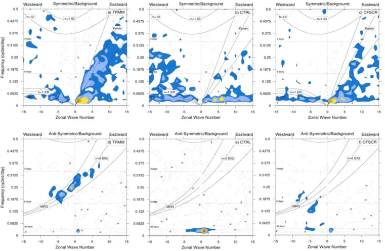
Figure 1.Wavenumber versus frequency distribution of spectral-power divided by estimate background spectra for (a–c) equatorially symmetric and (d–f) antisymmetric precipitation anomalies for observation (TRMM 3B42), CTRL and CFSCR. Shallow water dispersion relationships for equivalent depths of h512, 25, and 50 m are shown in black lines. Contour shading begins at 1.1 for which the spectral powers are 95% significant over the background spectra.
2015;Abhik et al., 2016] have found that the spectral ratio between eastward and westward propagating components of the CCEW could be crucial for BSISO simulation. Thus, it is worthwhile to investigate how reasonably the CCEWs have been simulated in CFSCR. Figure 1 assesses the distribution of CCEWs in wavenumber-frequency spectra for observed and simulated precipitation data sets during boreal summer, followingWheeler and Kiladis[1999]. In observations (Figure 1a), symmetric spectral peaks are evident for the low-frequency MJO (wavenumber 1–3 and periodicity about 45 day), n51 ER and high-frequency Kelvin, and n51 inertio-gravity (IG1) waves. In CTRL, all the symmetric waves are found to be weaker and disorganized (Figure 1b). The MJO spectral peak is also weakly simulated and it is shifted to a higher wave-number than in observations. Among the symmetric CCEWs, the most prominent improvement is noted in the simulation of MJO power by CFSCR (Figure 1c) relative to CTRL. However, marginal improvement is not-ed in the simulation of the high-frequency Kelvin waves over that in CTRL.
The distribution of equatorially antisymmetric precipitation spectral peaks is shown in Figures 1d–1f. In observations, significant spectral peaks corresponding to mixed Rossby gravity (MRG) and eastward inertia gravity (EIG) waves are present. A weaker peak corresponding to tropical disturbances is also evident around wavenumber25 and frequency 0.25 cycles per day. In CTRL, both the MRG and the EIG are severely underestimated (Figure 1e). The peak associated with the tropical depressions is less organized and shifted toward lower frequencies. On the contrary, the antisymmetric MJO signal is too strong in CTRL. The unusual antisymmetric MJO peak in CTRL is significantly reduced in CFSCR (Figure 1f). However, the simulation of the antisymmetric MRG and EIG does not improve in CFSCR. Only a weak organization of tropical depression-type disturbances begins to emerge around wavenumber25 and frequency 0.25 cycles per day in CFSCR.
As the subseasonal variability during boreal summer exhibits complex eastward and northward propagating modes, we analyze the spatiotemporal characteristics of eastward and northward propagating BSISOs. Fig-ure 2 shows the lag correlation analysis of 20–100 day filtered precipitation (shaded) and U850 (contour) against a base time series of 20–100 day filtered boreal summertime precipitation averaged over EEIO (East-ern Equatorial Indian Ocean; 108S–58N, 758–1008E). The correlation based on the time series of 20–100 day filtered precipitation anomalies over EEIO highlights the eastward (top plots, Figures 2a–2c) and dominant northward propagating BSISO events (bottom plots, Figures 2d–2f) which are associated with the eastward propagation. Compared to observations (Figure 2a), CTRL simulates a slower eastward propagation of BSISO convection over IO and the correlation rapidly decays across the Maritime Continent (Figure 2b). However,
Figure 2.Longitude (latitude) versus lag correlation of 20–100 day filtered precipitation (shaded) and U850(contour) with a base 20–100 day filtered precipitation time series over EEIO
U850anomalies show some eastward movement over the WP. In contrast, the eastward phase speed of the CFSCR-simulated BSISO matches well with the observations (Figure 2a). The convective anomalies propa-gate into the WP, but lower correlations are evident to the east of the Maritime Continent. Consistently, CFSCR-simulated U850anomalies also exhibit the observed phase relationship during eastward propagation over the WP.
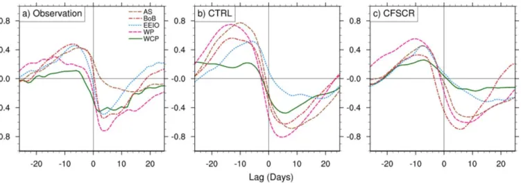
The quadrature relationship between precipitation and U850 is also evident for the observed northward propagating mode of BSISO over the ISM region (Figure 2d). The precipitation anomalies propagate north-ward from the equatorial region. The observed northnorth-ward moving BSISO appears to be stronger, slower, and of longer duration relative to the southward component. Unlike the eastward propagating mode, CTRL simulates the northward propagating mode to some extent (Figure 2e). But the simulated northward propa-gation appears to be slower than observed and the correlation decays rapidly away from the equator. In addition, the simulated southward propagation is considerably underestimated in CTRL. CFSCR produces a more realistic northward movement with the observed phase speed and temporal duration (Figure 2f). The amplitude of the northward propagating mode is comparable to the observations but the southward move-ment appears to be slower. The above analyses demonstrate that CFSCR reproduces most of the salient fea-tures of the eastward and northward propagation over the ISM region and also over the WP region. As the CFSCR has showed improvement in eastward and northward propagation, it will be worthwhile to investigate the ocean-atmospheric coupling in the CFSCR as compared to observations and CTRL. Earlier studies [e.g., Roxy and Tanimoto, 2012; Sharmila et al. 2013; here after S13] identified that the ocean-atmosphere coupling is overestimated over the Indian Ocean in the model. To examine how this coupling influences the local precipitation distribution, a lag correlation analysis between SST and precipitation is performed over the Indo-Pacific regions during JJAS (Figure 3). In Figure 3, ‘‘day 0’’ represents the day of maximum precipitation activity over the region of concern. The magnitude of the correlation indicates the intensity of the ocean-atmosphere coupling, while the lag-day refers the timescale that it takes the atmo-sphere to respond to the SST anomalies or vice-versa [Roxy and Tanimoto, 2012;Kumar et al., 2013]. In gen-eral, the leading warm SST anomalies drive the atmospheric convection which causes enhanced precipitation and cooling of the oceanic mixed layer by decreasing the shortwave fluxes to the surface under cloudy conditions. However, among these basins, some differences are observed in the response timescales [Roxy and Tanimoto, 2012]. Realistic simulation of this response is crucial for simulating subseaso-nal variabilities in current climate models [Wu et al., 2008]. The ocean-atmosphere-ocean feedback is well maintained both in CTRL and CFSCR over all the regions. As there is no apparent mismatch between the SST and precipitation in the model, it can be implied that the dynamical responses associated with the ocean-atmosphere coupling is reasonably captured in both the simulations. However, consistent with the results inRoxy[2014], the SST-precipitation relationship is found to be amplified over all basins in CTRL.
Figure 3.Lag-correlation of SST and precipitation anomalies over Arabian Sea (AS; 638–738E, 108–208N), Bay of Bengal (BoB; 808–908E, 108–208N), eastern equatorial Indian Ocean (EEIO; 758–1008E, 58S–108N), western Pacific (WP; 1208–1408E, 58–158N), and west-central Pacific (WCP; 1508E–1808, 108S–108N) during June–September from (a) Observation (TMI SST and TRMM rainfall), (b) CTRL, and (c) CFSCR. A positive (negative) lag corresponds to the situation when the precipitation anomalies lead (lag) the SST anomalies.
This overestimation is argued to be responsible for the amplification of the subseasonal variability over the ISM region [Roxy and Tanimoto, 2012]. This amplification of the SST-precipitation relationship is found to be considerably reduced as one moves from CTRL to CFSCR. An exception is the west-central Pacific where the negative correlation is relatively less at positive lags. It suggests a weaker atmospheric response to the local SST forcing leading to the SST warming over this region. However, this bias of CFSCR is mostly confined to the local relationship over the west-central Pacific as the SST-precipitation relationship in seasonal and sub-seasonal timescales is fairly well simulated over the other regions. Regardless of this discrepancy, it provides a favorable background for simulating better BSISOs in CFSCR over the Indo-Pacific regions.
The above analyses show the improved eastward and northward propagation of BSISOs and SST-rainfall relations over Asian Monsoon domain. Earlier studies [Chattopadhyay et al., 2009] showed that the north-ward propagation of BSISOs during boreal summer is promoted by the stratiform (large-scale) rainfall— contributed by the cloud microphysics scheme of the model. As the WSM6 scheme generates all types of cloud hydrometeors and the modification of critical radius improves the rain efficiency in CFSCR, it will be interesting to explore whether the large-scale rain in CFSCR shows the observed features. We, therefore, investigate how the improvement in the BSISO propagation characteristics is associated with an improve-ment in the large-scale rainfall in CFSCR. Previous studies [e.g.,Fu and Wang, 2004;Jiang et al., 2015] noted the importance of the top heavy heating profile [Schumacher and Houze, 2003] associated with large-scale precipitation on the propagation characteristics of the intraseasonal variability.Chattopadhyay et al. [2009] demonstrated that the northward propagation of BSISO is dominantly contributed by the anomalous response of the atmosphere to stratiform heating in the backdrop of mean easterly vertical shear. They have also emphasized that major drawbacks of climate model in capturing the northward propagation is attributed to the inability of simulating the stratiform (large-scale) component of total rainfall. To illustrate the role of individual precipitation components on the northward propagating BSISO, the total rainfall anomalies are decomposed into convective and large-scale components. It may be noted that different def-initions are used to partition the observed convective and stratiform rainfall. However, as the convective and large-scale rainfall simulated by both the models is directly comparable, we decided to compare between these two. The contribution of both the simulated rainfall categories on northward propagating BSISO convection is depicted in Figure 4. As a precaution, no direct comparison with the observation has
Figure 4.Latitude versus lag correlation of 20–100 day filtered convective and large-scale precipitation with same base precipitation timeseries as in Figure 2, based on CTRL and CFSCR.
been applied in this diagnosis. The Hovm€oller diagrams in Figure 4 are obtained from the same lag-correlation approach as in Figure 2. The convective and large-scale rainfall anomalies largely capture the northward propagating BSISO signal over the ISM region in both the simulations. However, the contribution of the large-scale rainfall is found to be weaker than the convective precipitation in the CTRL (Figures 4a and 4b). In contrast, comparable contributions from both the rainfall categories are noted in CFSCR (Figures 4c and 4d). This improvement in large-scale rainfall could be attributed to the contributions of cloud hydro-meteors in CFSCR, as revealed in Figures 12–15. This result suggests that the interaction between grid-scale and the subgrid-scale precipitation processes has improved in CFSCR and as a consequence, CFSCR simu-lates a more realistic northward propagation of BSISO.
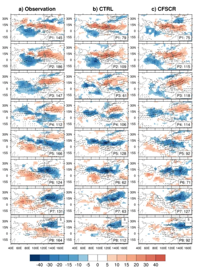
To provide more quantitative evaluation of the simulated BSISO organization, MvEOF analysis [Lee et al., 2013] is employed to extract the BSISO modes. The leading two PCs (PC1and PC2) from MV-EOF analysis are associated with BSISO1 mode that represents the spatiotemporal evolution of canonical northward and eastward propagating low-frequency intraseasonal variability. The spatial composite of OLR and wind anomalies further indicates the ability of the model to simulate the BSISO1mode. Figure 5 represents the JJAS composite OLR and wind anomalies at 850 hPa for observations and the model associated with BSISO1 mode. The corresponding phase space is divided into eight phases based on the BSISO1index, as inLee et al., [2013]. In observations, the convective signal (represented by negative OLR anomalies) first appears over the western equatorial IO at phase 1 and slowly propagates eastward (Figure 5a). At phase 3, the BSISO1signal further intensifies and reaches over EEIO. It further bifurcates in meridional directions, while another branch continues its eastward progression across the Maritime Continent up to the WP. The south-ern branch of the convection rapidly decays, while the northsouth-ern component slowly propagates toward the Indian subcontinent. The combination of eastward and northward movement of the BSISO convection results in a northwest-southeast tilting structure of organized BSISO convection (phase 4–5). During phase 4–5, the northward propagating enhanced convective anomalies reside over central India, and lead to an ‘‘active’’ spell of the ISM. The enhanced convective signal is further replaced by suppressed convection (rep-resented by positive OLR anomalies) in subsequent phases. CTRL reasonably reproduces some of the salient features of the observed BSISO1mode (Figure 5b). However, the organization of the convection is weak in CTRL and the simulated convection is zonally oriented rather than tilted. Additionally, the northward propa-gation of the BSISO1convection appears to be slowed down during phase 5. On the contrary, CFSCR cap-tured many of the salient features of the observed BSISO1 characteristics (Figure 5c). The simultaneous eastward and northward propagation are reasonably captured in CFSCR. This improvement might be responsible for the realistic intraseasonal variability of the enhanced convective anomalies and its realistic phase speed over the ISM region in CFSCR.
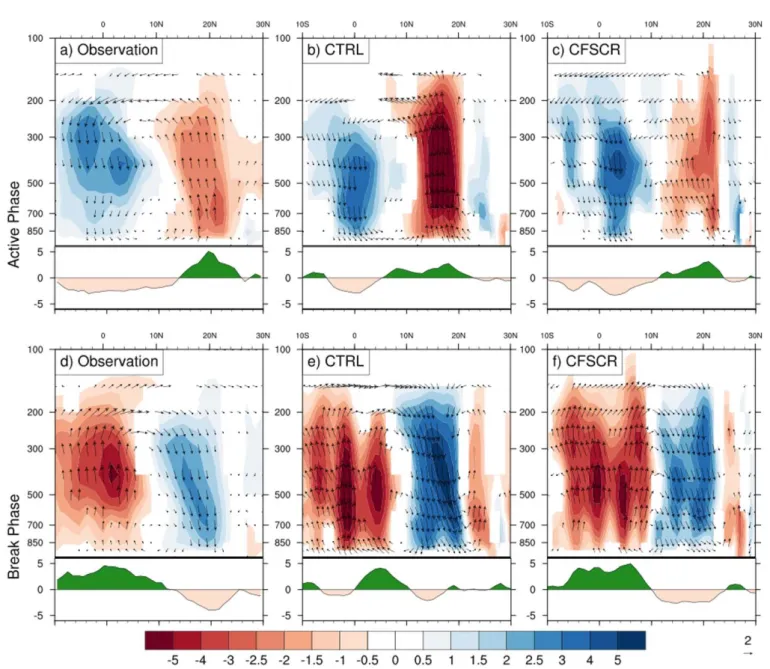
The diabatic heating associated with the northward propagating BSISO convection induces a large-scale monsoon circulation [Jiang et al., 2011;Abhik et al., 2013]. The vertical distribution of the diabatic heating considerably influences the structure of the regional Hadley circulation over the ISM region. In Figure 6, the anomalous Hadley circulation associated with the active (phase 4 of BSISO1) and break phase (phase 8 of BSISO1) of the ISM are examined. The corresponding meridional distribution of composite rainfall anomalies at the same BSISO phase is also displayed on the lower part of each plot. Figure 6a shows that the observed ascending (descending) branch of the regional Hadley circulation is located over the Indian latitudes (EEIO region) during the active phase. In CTRL, the ascending branch of the Hadley circulation is too strong and confined to the south of 208N, the location of the usual monsoon trough (Figure 6b). The corresponding rainfall activity is found to be weak beyond 208N. It appears that CTRL-simulated organized BSISO convec-tion fails to propagate beyond 208N. As a consequence, the north-south ‘‘dipole’’ structure is also not well represented in CTRL. Interestingly, this bias of the model is reduced in the CFSCR simulation. Both the amplitude and the structure of the regional Hadley circulation are reasonably simulated in CFSCR (Figure 6c). The north-south precipitation dipole is also realistically captured in CFSCR during the active phase. During the break phase, the observed anomalous Hadley circulation reverses its direction (Figure 6d). The corresponding ascending (descending) branch is located over the EEIO (Indian latitudes). Consequently, the enhanced (decreased) precipitation anomalies are also shifted to the EEIO (Central India) region. The CTRL-simulated anomalous Hadley circulation is too strong and disorganized relative to observations (Figure 6e). The lack of organization can be noted in corresponding precipitation anomalies as well. In contrast, CFSCR produces a realistic north-south dipole structure and organized BSISO convection (Figure 6f). The revision of
Figure 5.The life-cycle composite of OLR (shaded, W m22) and 850 hPa wind (vector, m s21) anomalies reconstructed based on PC1 and PC2 of BSISO1 in eight phases. Composited anomalies below 95% level of significance are masked out. The number of days used to generate the composite for each phase is shown to the right-bottom corner of each plot.
the convective processes in the model appears to have great impact on the spatiotemporal distribution of the BSISO convection.
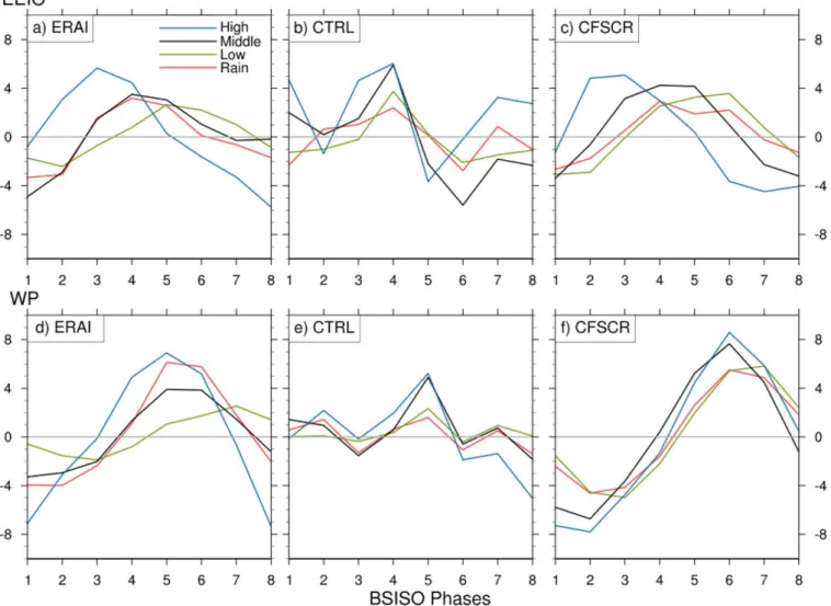
To understand the role of interaction between cloud processes and the large-scale BSISO circulation, the phase-relationship of the various cloud (low, medium, and high) distributions associated with BSISO1 con-vection (represented by precipitation anomalies) are examined over both the EEIO (top plots) and WP (bottom plots) regions (Figure 7). In the observations, the transition from low to middle to high cloud is evi-dent during BSISO evolution over the EEIO (Figure 7a) and WP (Figure 7b). The low cloud anomalies lead the maximum BSISO convection, while the high cloud peak lags the maximum convection. A similar cloud evolution associated with BSISO was already reported in earlier observation-based studies over the ISM region [e.g.,Jiang et al., 2011;Abhik et al., 2013]. However, CTRL does not produce such a relationship over the EEIO and WP, low cloud maxima collocate with the maximum BSISO rainfall activity (Figures 7c and 7d, respectively). This indicates a lack of preconditioning processes at the leading edge of the simulated BSISO convection due to the occurrence of precipitating low clouds. As a result, a considerable amount of the rain-fall is produced by the premature convection in the model. This problem of the model is consistent with
Figure 6.Anomalous Hadley circulation associated with (top) active (phase 4) and (bottom) break (phase 8) conditions. Composited anomalies below 95% level of significance are masked out. At lower part corresponding rainfall anomalies (mm d21
the overestimation of the lower rain-rate in the model over these two regions (figures not shown). In con-trast, the vertically tilted cloud structure is well reproduced in CFSCR over EEIO (Figure 7c). The realistic BSISO propagation over the EEIO region is likely to be related to a reasonable simulation of the trimodal cloud distribution [Johnson et al., 1999;Jiang et al., 2011;Abhik et al., 2013] in CFSCR. The better cloud-type distribution in the model is attributed to the use of a robust cloud microphysics (WSM6) scheme that pro-duced cloud hydrometeors such as cloud water, graupel, snow, cloud ice for the formation of shallow, con-gestus, and deep clouds. In contrast, the gradual growth of the convection is moderately simulated in CFSCR over the WP (Figure 7f). This limitation of CFSCR is consistent with the simulation of weak eastward propagation over the WP, as shown in Figure 2c.
3.2. Improvement in Mean State of Summer Monsoon
The capability of a model to simulate the realistic intraseasonal variability is intimately associated with its ability to simulate the mean climate [Slingo et al., 1996;Waliser et al., 2003;Yang et al., 2012]. In view of the importance of the seasonal mean state, an assessment of the simulated mean state is provided in this sub-section. A realistic simulation of the ISM largely depends on the fidelity of the model to simulate the large-scale mean state [Sperber et al., 2013;Goswami et al., 2015]. Figure 8 shows the seasonal mean precipitation (in mm d21, top plots) and the SST (in
8C, bottom plots) distributions for observations (TRMM and TMI, respectively) and the difference between CTRL and observation, CFSCR and observation, and CFSCR and CTRL. The observed precipitation maxima during boreal summer are located over the Western Ghats, along
Figure 7.Evolution of anomalous low, middle, and high cloud fractions (%, left axis) and rainfall anomalies (mm d21
, right axis) associated with BSISO1convection over (top) EEIO and
Figure 8.(top) Seasonal (June–September) mean precipitation (in mm d21) for (a) observation (TRMM) and the bias in (b) CTRL and (c) CFSCR relative to the observed seasonal mean precipitation and (d) the difference in seasonal mean precipitation between CFSCR and CTRL. (bottom) Same as in the top plots, but for seasonal mean SST (in8C) for observation (TMI), CTRL, and CFSCR. The precipitation and SST biases which are significant at the 95% level using a student’sttest, are only shown.
the eastern shore of the Bay of Bengal (BoB), and over the WP, near the Philippines (Figure 8a). A secondary precipitation maximum is also seen over the EEIO. TMI-based seasonal mean SST displays maxima (298C) over the EEIO, head BoB, and WP warm pool region. Although CTRL captures the location of the observed precipitation maxima (Figure 8b), the precipitation amount is considerably overestimated (underestimated) over the equatorial Indian Ocean (Indian landmass) region. Consistent with previous studies (e.g., S13; G14), the simulated tropical SST is found to be colder than observed, especially over the Indian Ocean (IO) in CFSv2 (Figure 8f). In contrast, CFSCR shows a better agreement with the observed precipitation distribution over the ISM domain (Figure 8c). The locations of the SST maxima are also reasonably simulated in CFSCR (Figure 8g).
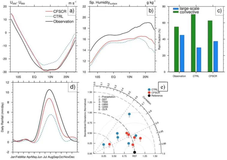
The relative difference in mean precipitation and SST distributions between CFSCR and CTRL are shown in Figures 8d and 8h. Both the dry bias over the Indian land and wet bias over the IO have reduced in the CFSCR simulation. In addition, the double ITCZ problem over the WP regions in CTRL has been considerably improved. The improvement in the precipitation distribution in CFSCR is not only limited to the Indo-Pacific warm pool region, but the improvement is also evident over equatorial Africa and northern America (Figure 8d). The colder SST bias of CTRL has reduced in CFSCR over the tropical oceans, especially over the IO (Fig-ure 8h). However, the simulated precipitation band over the Pacific is too strong in CFSCR relative to the observation and it extends up to the eastern Pacific. Comparing all the analyses of mean rainfall and SST, the RMSE of CFSCR is found to be less than CTRL suggesting relative improvement of the JJAS mean. Earlier studies [e.g.,Jiang et al., 2004; S13;Abhik et al., 2014] suggested that the realistic simulation of the atmospheric internal dynamics is a key to simulate mean state of the ISM and its intraseasonal variability. Jiang et al. [2004] also demonstrated that the interaction between seasonal mean low-level moisture and the mean flow contributes to the moisture convergence to the north of the BSISO convection. The seasonal mean vertical easterly wind shear (difference between zonal wind at 200 and 850 hPa) plays an important role in inducing barotropic vorticity ahead of the northward propagating BSISO convection [Jiang et al., 2004]. Figure 9a shows the meridional distribution of observed and simulated vertical easterly shear during JJAS. The observed easterly shear maxima is found to be located around 108N and its amplitude is consider-ably strong over the ISM region. The vertical wind shear appears to be weakly simulated in CTRL. In contrast, CFSCR better simulates the amplitude and distribution of the easterly shear over the ISM region.
The meridional asymmetry of the summer mean moisture distribution is also considered to be crucial for the northward movement of the BSISO convection [Jiang et al., 2004]. In Figure 9b, the JJAS mean observed surface-specific humidity maximum is found to be located around 208N over the northern IO. But, CFS shows a limitation in simulating the seasonal mean-specific humidity field at the surface. In both the simula-tions, the meridional gradient of mean surface moisture is weaker compared to the observation. However, CFSCR exhibits a marginal improvement over CTRL in simulating meridional moisture gradient.
Further, the simulated total rainfall is partitioned into two categories: convective (subgrid-scale) and large-scale (grid-large-scale or resolved-large-scale) precipitation. Previous observation based studies [e.g.,Schumacher and Houze, 2003] suggested that the stratiform precipitation exhibits a top-heavy heating structure and plays a major role in the propagation and maintenance of the tropical intraseasonal convection [Fu and Wang, 2004;Chattopadhyay et al., 2009;Deng et al., 2015]. A similar top heavy latent heating profile is usually asso-ciated with grid-scale or microphysical precipitation [Fu and Wang, 2009;Jiang et al., 2015]. Observed and simulated convective stratiform rainfall ratios are shown in Figure 9c. Similar overestimation (underestima-tion) of the convective (large-scale) rainfall, as in CTRL, is found to be present in CFSCR. However, the ratio of these two rainfall categories has improved in CFSCR.
The annual cycle of the rainfall distribution over the ISM domain exhibits the seasonal migration of the ITCZ [S13; G14;Goswami et al., 2015] and a realistic simulation of this annual cycle is considered to be a challenge for the current GCMs [Sperber et al., 2013]. As in the earlier section, the simulation of BSISOs is found to have improved, and it will be interesting to explore whether the annual rainfall cycle over central India (738–858E, 158–258N) also shows an improvement. Figure 9d shows the seasonal migration of the rain-band during boreal summer months in observations. Consistent with the results in Figure 8, the CTRL-simulated rainfall amplitude is too weak over this region. Additionally, it exhibits a late onset and an early withdrawal, thereby resulting a shorter rainy season in CTRL. CFSCR is found to improve the annual cycle over Indian region compared to CTRL.
The fidelity of the model in simulating the seasonal mean precipitation, wind at 850 and 200 hPa, tempera-ture at 500 hPa, OLR and SST over the ISM domain (408–1208E, 158S–308N) is shown in a Taylor diagram [Taylor, 2001] (Figure 9e). Consistent with previous figures, the CFSCR shows better correlation and variabil-ities for most of the parameters. However, the underestimation of the SST variability in CTRL is marginally resolved in CFSCR simulation.
To further investigate the reason behind the improvement of the mean rainfall distribution in CFSCR, the feedback between moisture and convective processes is diagnosed in Figure 10. This figure shows the com-posite relative humidity profile over the ISM domain (408–1208E, 158S–308N) as a function of rainrate [Thayer-Calder and Randall, 2009;Del Genio et al., 2012]. For better readability, bias profile from the simula-tions is contoured over the corresponding profile. In Figure 10a, the observed profile indicates a moist col-umn for moderate and higher rainrates. In contrast, the middle troposphere is found to be dry for the lower rainrates. This result suggests that the lower tropospheric relative humidity is more sensitive for the lower rain rates. The observed moisture distribution is largely represented in both the simulations. However, CTRL simulates relatively dry layers for lower rainrate (Figure 10b). It indicates that the lower rainrates are less sensitive to the available moisture in CTRL. In CFSCR, the moisture profile is more realistic (RMSE is 8.7% rel-ative to that is 9.2% in CTRL) than that in CTRL, especially for the lower rainrates (Figure 10c). But an overly moist column relative to the observed profile is noted for higher rainrates. This feature is not uncommon in current climate models.Thayer-Calder and Randall[2009] also previously reported similar overmoistening cases due to excessive evaporation and moisture convergence during intense rain events in SP-CAM.
Figure 9.Meridional distributions of boreal summer mean (a) Ushear, (b) surface Sp. Humidity for observation, CTRL, and CFSCR. All data set are averaged between 708E and 908E.
(c) convective and large-scale rain fraction (%) over the ISM region (408–1208E, 158S–308N), (d) Climatological annual precipitation cycle over central India (738–858E, 158–258N), (e) Taylor diagram for summarizing the relative skill of the simulations relative to the observed summertime mean meteorological fields over the same ISM region as in Figure 9c. Black dot denotes the reference point.
However, better lower tropospheric moistening in CFSCR helps to sustain a proper moist static stability in the environment. Along with improvement of low level moisture, the modification of critical cloud droplet radius (rcr) in the autoconversion process with a more realistic value (10lm) could be one of the key factors for the improvement of rainfall as evident in Figure 9c and 9d. The CFS model even with less moisture gen-erates substantial rain as the smaller critical cloud droplet radius (rcr) initiates rain formation more frequently than that of CFSCR where the rain drop has to grow up to the size of 10lm to eventually initiate the rain. We have intended to improve the cloud processes by incorporating an advanced microphysical scheme in CFSv2. To quantify whether the right types of cloud (low, middle, deep) are causing the right rainfall categories, a joint probability density distribution (PDD) of OLR and precipitation is made over the domain 158S–308N, 508–1108E (Figure 11). This analysis will bring out whether the model is producing realistic rainfall distribution from appropriate cloud categories, as in the observation. It answers the ques-tion whether the model produce too much rain due to lack of growth of deep clouds or the model has too much of deep clouds and associated heavy rain rates. Based on similar analysis,Goswami et al. [2015] showed that the cloud-rain relationship improves in the superparameterized CFS. In this analysis, an OLR data set is used as a proxy for convection. All rainfall events are counted into 6 mm d21bins and the OLR values are classified in 10 Wm22bins. The joint PDD indicates the contribution of the rainfall/OLR distribu-tion (expressed in %) in a particular bin for the entire period. The PDD of CTRL (Figure 11a, contour) could not capture the observed (shaded) relationship between OLR and the rainfall distributions. Particularly, the CTRL could only simulate a minimum OLR195 Wm22as against 180 Wm22in the observation. The rainfall and OLR distribution does not match well even in the lower rainfall category from shallower cloud (with OLR between 260 and 300 Wm22). The PDD of CFSCR (Figure 11b) considerably improves the OLR and rainfall relation against the observation. This improvement indicates that a better representation of the prognostic cloud variables by WSM6 in CFSCR led to a realistic simulation of cloud-rainfall distribution.
Although we have discussed the cloud-rainfall relationship in terms of OLR, we feel, quantification of the contribution of different hydrometeors to different rainfall categories will be important in the light of improvement of rainfall variabilities particularly the stratiform component. Figures 12a–12d shows the impact of cloud hydrometeors (cloud ice and cloud water) on simulated total and large-scale rainfall (mm d21) over the central Indian region (73
8–858E, 158–258N). It is evident from Figures 12a and 12b that the cloud ice (CLI) has a maximum at around 250 hPa and it dominantly contributes to the lighter and moderate rainfall categories. The contribution of cloud water (CLW) on different categories of total rain rate is shown in Figure 12c, while the impact of CLW on large-scale rain rate is assessed in Figure 12d. Cloud water (Figures 12c and 12d) appears to increase in the lower troposphere (below 500 hPa) for rainfall above 100 mm d21. CFSCR-simulated cloud ice contributes in the lighter and moderate
Figure 10.Composite profile of relative humidity as a function of rain rate over the ISM domain (408–1208E, 158S–308N) during all JJAS seasons from (a) observation (ERA-Interim versus TRMM), (b) CTRL, and (c) CFSCR. The rain rate at thexaxis is plotted in log10scale. The bias in the simulated profiles relative to the observation are shown in contour (10b and 10c), while
categories of large-scale rainrate, which is analogous to the observed stratiform rain. The model simulat-ed CLI and CLW distributions and their relationship with the rainfall distribution are consistent with recent TRMM 2A12-based observations [Bhattacharya et al., 2014].
To get further insight into the contribution of various cloud hydrometeors (namely the CLW, CLI, and the mixed phase—snow and graupel) to large-scale (stratiform) rainfall, the vertically integrated hydrometeors
Figure 11.Joint probability density distribution (PDD) of daily OLR (Wm22
) and rainfall (mm d21
) during JJAS period for (a) CTRL and (b) CFSCR over the region 508–1108E, 158S–308N. The observed (AVHRR OLR and TRMM rainfall) distribution is indicated in shade at each plot.
and rainfall scatter plots over the ISM region is shown in Figures 13a–13c. These plots show the percentage contribution of each vertically integrated hydrometeor for a particular category of large-scale rainfall. Figure 13a shows the relation of vertically integrated CLI with the large-scale rainfall. It is evident that lower values of CLI contribute around 50–60% to the lighter rain rate and higher values of CLI contribute around 15–20% for the higher rain-rate categories for the large-scale rainfall. This allows a quantitative assessment between large-scale rainfall and the mixed phase hydrometeors (Figures 13b) in a climate model. Figure 13b shows that the mixed-phase hydrometeors having mixing ratio0.05 kg m22contribute around 70% in almost all categories of large-scale rainfall. However, for the higher rain rates, the percentage contribution from higher amounts of mixed phase is found to be around 15–20%. The generation of these hydrometeors by WSM6, thus, contributes in improving the proportion of large-scale rainfall, largely consistent with results in Figure 9c. In contrast, CLW contributes to the large-scale rain with much lesser magnitude (Figure 13c) relative to the contribution of CLI and mixed phase. The range of vertically integrated CLW contributing to the large-scale rainfall lies within 0–0.18 kg m22. These analyses quantify the role of hydrometeors and their contribu-tion in the simulated large-scale rainfall and provide the basis behind the improvement of large-scale (strat-iform) rainfall in CFSCR over the ISM region.
Figure 12.Vertical distribution of CLI (mg kg21
) as a function of (a) total precipitation and (b) large-scale precipitation over Central India (CI) during JJAS of CFSCR. (c and d) Same as in Figures 12a and 12b, but for CLW (mg kg21
). The total and large-scale precipitation values have been grouped into 10 mm d21
Waliser et al., [2009] emphasized that simulating realistic global distri-bution of cloud hydrometeors in current GCMs is also one of the long-standing challenges. Although the relation of hydrometeors with large-scale and total monsoon rain-fall has been highlighted, the ques-tion may be asked whether the improvement is happening locally or whether the modification of cloud microphysics in CFSv2 captures the global mean spatial and vertical dis-tribution of CLI and CLW as well. We compare the vertical distribution of CLI and CLW in CFSCR relative to the Cloudsat observations. Figure 14 shows the zonally averaged, vertical-meridional distribution of CLI during JJAS from CloudSat and CFSCR. In Figure 14a, the vertical structure of CloudSat CLI depicts primary maxi-ma around 275 hPa over the tropics, associated with deep convection and two secondary maxima around 500 hPa along the midlatitude storm tracks in both the hemispheres. The simulated CLI (Figure 14b) largely represents the observed structure but with slight overestimation throughout the latitude belt. Howev-er, the simulated tropical convection (from south of equator to 308N) appears to be reasonably simulated in CFSCR relative to CloudSat. The CLI distribution in CFSCR could be overestimated as CloudSat CPR is inherently less sensitive to the thin Cirrus generally observed near the Tropopause. However, the CFSCR exhibits notable bias (with mean bias of 2.1 mg kg21and root mean square error of 6.7 mg kg21) in simulating lower tropospheric CLI beyond 608 latitudes in both the hemispheres, especially in the south-ern hemisphere. Although CFSCR reasonably simulates the vertical structure with a moderate RMSE, the simulated variability appears to be lower than the observation.
Similarly the JJAS mean meridional-vertical distribution of CloudSat and CFSCR CLW are shown in Figures
Figure 13.Vertically integrated seasonal (JJAS) mean (a) cloud ice (kg m22), (b) mixed phase (snow and graupel) hydrometeors (kg m22
), and (c) cloud liquid water (kg m22
) as a function of large-scale precipitation (mm d21). The precipitation rate at thexaxis is plot-ted in log10scale. All data set is averaged over the ISM region (408E–1208E, 158S–308N).
14c and 14d, respectively. The simulated CLW broadly captures the vertical distribution of observed CLW. However, CFSCR overestimates CLW over the midlatitudes, around 458in both the hemispheres. Over the tropics, it extends vertically up to 600 hPa as against 400 hPa in the CloudSat (Figure 14c). The variability of CLW is reasonably simulated in CFSCR (contours in Figure 14d) with an RMSE of 8.1 mg kg21, while its bias is found to be 0.1 mg kg21.
To get further insight about the global spatial hydrometeor distributions, observed and simulated CLI at 275 hPa (Figures 15a and 15b, respectively) and CLW at 850 hPa (Figures 15c and 15d, respectively) are
Figure 14.Zonally averaged seasonal (JJAS) mean vertical-meridional distribution of (a) cloud ice water (CLI) content (mg kg21
) from CloudSat and (b) CLI from CFSCR; (c) cloud liquid water (CLW) content (mg kg21
) from CloudSat and (d) CLW from CFSCR. The seasonal (JJAS) standard deviation (mg kg21
) values are shown in contour and the CFSCR bias and RMSE values (mg kg21
) are mentioned at the upper right corner of the corresponding plots.
examined. CFSCR broadly captures the spatial distribution of CLI and CLW as compared to CloudSat, although the model overestimates the magnitude of CLI over eastern China, north-west Pacific, Maritime Continents, and also over the southern equatorial Pacific Ocean regions. CFSCR is able to capture the observed CLW distri-bution over the globe, except the underestimation over northern high latitudes, the eastern Pacific and Atlan-tic marine stratocumulus regimes. Simulation of global mean cloud ice and cloud water by a climate model is a long standing issue, and this study attempts to resolve the issue of representing the low level CLW, middle level mixed phase and upper level CLI in a climate model. The reasonable simulation of global mean trimodal cloud types are also consistent with the trimodal cloud types associated with the BSISO phases in Figure 7. This improvement in large-scale rainfall could be attributed to the contributions of cloud hydrometeors as revealed in Figures 12–15. Additionally, CFSCR-simulated precipitation anomalies show better organization.
This result suggests that the interaction between grid-scale and the subgrid-scale precipitation processes has improved in CFSCR and as a consequence, CFSCR simulates a more realistic northward propagation of BSISOs.
Last, we evaluate the cloud radiative effect in CFSCR relative to CTRL and the observation. CFSCR shows an improvement of short wave flux over the southern hemisphere as compared to the performance of CFS
Figure 15.Seasonal (JJAS) mean Cloud ice water (CLI) content (mg kg21
) at 275 hPa from (a) CloudSat, (b) CFSCR. Seasonal mean spatial cloud liquid water (CLW) content (mg kg21
) at 850 hPa from (c) Cloudsat, (d) CFSCR. The seasonal standard deviation (mg kg21
) values are shown in contour and the CFSCR bias and RMSE values (mg kg21
relative to the CERES observation. CFSCR shows marginally higher short wave flux over the Indian region, while over the northern latitudes, both the CFSCR and CTRL show similar variation (Figure 16a). The OLR dis-tribution (Figure 16b) in CFSCR shows some improvements over the Indian latitudes which could be attrib-uted to the simulation of better cloud classification in CFSCR due to improved cloud process parameterization through WSM6. In general, both the simulations show similar variation of net short wave flux at the TOA with marginal improvement in CFSCR over southern latitudes and some improvement of OLR over Indian latitudes.
4. Summary and Conclusions
A precipitation physics package with a revised convective parameterization and a new microphysical scheme has been implemented in NCEP CFSv2. The primary objective of this revision is to improve the per-formance of the model in simulating boreal summer-time mean climate and intraseasonal variability over the Indo-Pacific region by incorporating more realistic microphysical processes. Earlier studies [e.g.,G14; Abhik et al., 2016] have indicated that the convective processes are the major source of systematic biases in CFSv2. Some of these model biases, particularly the diurnal cycle, daily PDF and the seasonal mean precipi-tation, are found to be improved in the simulation of CFSv2 with the revised SAS convective scheme [Ganai et al., 2015]. In spite of these improvements, it still could not resolve the issue of a realistic ratio between convective and large-scale rainfall over the global tropics. A top-heavy latent heating profile in GCMs is usu-ally associated with large-scale precipitation and therefore is crucial for realistic simulations of BSISO. This suggests that the simplified microphysics [Zhao and Carr, 1997] in the model may not be sufficient to pro-duce realistic large-scale rainfall distribution and repro-duce the existing systematic biases of the model. To resolve these limitations of CFSv2, we have adopted similar revision of the existing convective parameteri-zation (SAS) in the model as inGanai et al., [2015]. Moreover, the Zhao-Carr microphysical scheme of the model has been replaced by the WSM6 scheme in the CFSCR simulation. Based on recent aircraft observa-tions during various campaigns over the Indian region, the critical threshold rain drop radius (rcr) is changed from 8 to 10lm in the WSM6 scheme for reducing too frequent rain initiation in the scheme.
The CFSCR-simulated mean climate shows substantial improvements over CTRL simulation during boreal summer. The rainfall distribution has been improved over the Indian land mass, EEIO, WP, equatorial Africa, Amazon basin, and northern America. In addition, the double ITCZ structure over WP appears to be improved in CFSCR. It may be noted that similar improvements in seasonal mean precipitation climatology
Figure 16.(a) Net short wave flux (W m22
) and (b) Net outgoing long wave radiation (OLR, W m22
) at the top of the atmosphere (TOA) based on observation (CERES), CTRL, and CFSCR.
have also been found by revising convective parameterization of the model inGanai et al. [2015]. This sug-gests that the majority of the simulated precipitation is contributed by the convective parameterization at T126 resolution. However, successful simulation of mean-state precipitation distribution is not sufficient to simulate a realistic monsoon variability [DeMott et al., 2011]. Realistic representation of the convective and large-scale precipitation ratio is argued to be crucial for the simulation of the tropical variability [Fu and Wang, 2004;Jiang et al., 2015]. This ratio has not been improved by revising the convective parameteriza-tion [Ganai et al., 2015], mainly due to lack of a robust grid-scale cloud scheme in the model. In contrast, CFSCR exhibits superior skill in simulating the ratio between convective and large-scale precipitation cate-gories relative to those inGanai et al. [2015]. The relative success of CFSCR, as seen in the rainfall PDF and other characteristics of the ISM, is likely due to the implementation of robust cloud microphysics scheme and a more realistic autoconversion process in WSM6. Although the replacement of the simple autoconver-sion ofSundqvist et al. [1989] by more physically based autoconversion [Hong and Lim, 2006;Tripoli and Cot-ton, 1980], has resulted in improvement in precipitation, there is a need of further research in evaluating other physical processes to ascertain the caveats of such complex parameterizations that are not mani-fested as compensating errors [Neggers and Siebesma, 2013] from other physical processes. Nevertheless, the systematic improvement in the three-dimensional structure of cloud and associated rainfall variability in CFSCR will be an excellent resource for the climate applications.
The more sophisticated cloud processes also affect cloud hydrometeor distributions in CFSv2. Interestingly, CFSCR reasonably captures both the vertical and horizontal distribution of CLW and CLI. The simulated CLW may further help to resolve the unusual lower tropospheric drying as in CTRL and could prevent the model from creating an environment that has negative moist static stability [Neelin and Held, 1987]. Realistic lower atmospheric moisture sensitivity for the lower and moderate rainrates could lead to a better precipitation distribution in CFSCR. Consistent with the improvement in the convective processes, other dynamical parameters are also found to be improved with the revised cloud processes. These improvements may arise from better feedback between convective processes and the large-scale circulation in the model.
CFSCR also shows its potential in simulating a realistic BSISO signal over the Indo-Pacific region. This variability is crucial for a realistic monsoon simulation in current climate models. Realistic simulation of the cloud hydrome-teors ensures a trimodal distribution of the tropical clouds [Johnson et al., 1999] in the model. The phase-relationship between CFSCR-simulated BSISO convection and the different cloud distributions show improve-ment relative to the observations [Jiang et al., 2011]. As a consequence, the eastward and northward propagating BSISO modes are realistically simulated with the observed phase-speed over the ISM domain. Such improvement may arise from the improvement of the ratio between convective and large-scale precipitation in CFSCR. Earlier studies [e.g.,Fu and Wang, 2004;Chattopadhyay et al., 2009] showed the importance of this ratio for maintaining the top-heavy heating profile during eastward and northward propagation. The inclusion of sophisticated micro-physical processes is favorable for improving the large-scale precipitation distribution in the model.
Although CFSCR shows improvements in reducing the systematic biases of CFSv2, a considerable wet bias remains over the equatorial central and eastern Pacific Ocean, which could be due to the warm SST bias over the region. It needs to be explored further whether such an overly warm SST could influence other slowly varying external forcings (e.g., El-Ni~no Southern Oscillation) in CFSCR. The cloud-precipitation relationship is also found to be weakly simulated over this region. This may lead to weakening of the simulated eastward propagation over the WP. The wet bias over the WP may further contribute to the precipitation biases in CFSCR through tele-connections. Although the total radiation at the top of the atmosphere by CFSCR does not show a substantial dif-ference with respect to CTRL, a detailed analyses [Ajayamohan et al., 2011;Crueger and Stevens, 2015] of cloud-radiative feedback with BSISO phases by the CTRL and the CFSCR will be attempted in the second part of the paper that follows up on some of these details. To reduce the existing biases in CFSCR, various sensitivity experi-ments would be useful in guiding future work. The quantitative estimation of the seasonal to subseasonal hind-cast skill and an evaluation of the interannual variability in CFSCR will be of great interest and these are left for future research. Some of these evaluations will also be discussed in the next part of this paper.
References
Abhik, S., M. Halder, P. Mukhopadhyay, X. Jiang, and B. N. Goswami (2013), A possible new mechanism for northward propagation of boreal summer intraseasonal oscillations based on TRMM and MERRA reanalysis,Clim. Dyn.,40, 1611–1624, doi:10.1007/s00382-012-1425-x.
Acknowledgments
This work is a part of PhD dissertation of S Abhik, financially supported by Council of Scientific and Industrial Research (CSIR), Govt. of India and Indian Institute of Tropical
Meteorology (IITM), Pune. IITM, Pune is fully funded by the Ministry of Earth Sciences (MoES), Govt. of India, New Delhi. Some of this research by S Abhik is also supported by Australian Research Council’s (ARC) Centre of Excellence for Climate System Science (CE110001028). Authors are grateful to Editor, the associate editor,
Christopher Bretherton and other two anonymous reviewers for their detailed review and constructive comments, which helped us to improve the quality of the manuscript. The CloudSat data were provided through CloudSat project of NASA. M.M. would like to thank Duane E. Waliser and Jui-Lin Franke Li, JPL/ CalTech for providing guidance and help in processing and analysing the data while the author was at JIFRESSE, UCLA as a visiting scholar sponsored under the National Monsoon Mission project, funded by MoES, Govt. of India. We acknowledge ECMWF for providing ERA-interim data set (http:// apps.ecmwf.int/datasets/data/interim-full-daily), NCEP for reanalyses data set (http://www.esrl.noaa.gov/psd/data/ gridded/data.ncep.reanalysis2.html), NOAA’s National Operational Model Archive and Distribution System (NOMADS) for CFSR data set (http:// nomads.ncdc.noaa.gov/modeldata/ cmd_pgbh/) and Goddard Earth Sciences (GES) Data and information service center (DISC) for TRMM dataset (http://precip.gsfc.nasa.gov/). The TMI SST data are downloaded from ftp:// ftp.remss.com/tmi/bmaps_v07.1/ y2014/m01/, while OLR data are made available by the NOAA/OAR/ESRL PSD, Boulder, Colorado, USA, at their website http://www.esrl.noaa.gov/psd/ . The CERES data set is obtained from the NASA Langley research centre atmospheric sciences data center (https://ceres.larc.nasa.gov/). We wish to thank NCEP for providing CFSv2 model through National Monsoon Mission and S. Moorthi, Jongil Han, and Ruiyu Sun, NOAA/NCEP for helpful discussion regarding CFSv2 development. The CFSCR model output used in this study is archived at IITM and can be accessed from the corresponding author upon request. Sharmila S is acknowledged for her internal review and editorial assistance. National Center for Atmospheric Research (NCAR) is duly acknowledged for making available NCAR Command Language (NCL).