AN EFFICIENT AND EFFECTIVE CONVOLUTIONAL NEURAL NETWORK FOR VISUAL PATTERN RECOGNITION
LIEW SHAN SUNG
AN EFFICIENT AND EFFECTIVE CONVOLUTIONAL NEURAL NETWORK FOR VISUAL PATTERN RECOGNITION
LIEW SHAN SUNG
A thesis submitted in fulfilment of the requirements for the award of the degree of Doctor of Philosophy (Electrical Engineering)
Faculty of Electrical Engineering Universiti Teknologi Malaysia
iii
iv
ACKNOWLEDGEMENT
The past three years has been one of the most challenging yet exciting journey for me, and I feel very grateful to be able to experience it first hand, while shaping myself to become a better person.
First and foremost, I would like to express my deepest gratitude to my dear supervisor, Prof. Dr. Mohamed Khalil Mohd. Hani for his encouragement, criticism, and love during my Ph.D. journey. His great enthusiasm for the research and philosophy of life have enlightened me in a significant way. I always look up to him not just being a mentor, but a role model, and a father.
My sincerest appreciation also goes to my former co-supervisor Dr. Rabia Bakhteri for her guidance and dedication towards my research work. Thank you Dr. and I wish you all the best in Canada. In addition, I would like to express my great appreciation to my internal and external examiners, Assoc. Prof. Dr. Muhammad Nadzir Marsono from Universiti Teknologi Malaysia and Prof. Dr. Raveendran a/l Paramesran from Universiti Malaya for their invaluable comments and commendation in evaluating my thesis. I would also like to convey my gratitude to Dr. Usman Ullah Sheikh for his comments and criticism during my Ph.D. proposal defense.
It was also a great privilege to work closely with my fellow seniors Dr. Jasmine Hau, Dr. Vishnu, Dr. Syafeeza, Moganeshwaran, Lee Yee Hui and Sia Chen Wei for their technical supports and advices. Not to forget the members of the VeCAD Research Laboratory: Alireza, Han Chien, Hui Ru, Ikmal, Jeevan, Jia Wei, Khang Hua, Ling Kim, Omid, Stephen, Vidya, and Yin Zhen. It would be a dull and lonely journey without your company.
Most importantly, I would like to thank my family, especially my dear parents for always being there for me, and for their love and patience. Thank you for the boundless supports to pursue my dream. Without exception, a special thanks to Evonne, for her unwavering love, devotion, support, and patience through these years, even at the times when I was in the state of depression or frustration. This Ph.D. journey would have been impossible without all of you. Thank you.
v
ABSTRACT
Convolutional neural networks (CNNs) are a variant of deep neural networks (DNNs) optimized for visual pattern recognition, which are typically trained using first order learning algorithms, particularly stochastic gradient descent (SGD). Training deeper CNNs (deep learning) using large data sets (big data) has led to the concept of distributed machine learning (ML), contributing to state-of-the-art performances in solving computer vision problems. However, there are still several outstanding issues to be resolved with currently defined models and learning algorithms. Propagations through a convolutional layer require flipping of kernel weights, thus increasing the computation time of a CNN. Sigmoidal activation functions suffer from gradient diffusion problem that degrades training efficiency, while others cause numerical instability due to unbounded outputs. Common learning algorithms converge slowly and are prone to hyperparameter overfitting problem. To date, most distributed learning algorithms are still based on first order methods that are susceptible to various learning issues. This thesis presents an efficient CNN model, proposes an effective learning algorithm to train CNNs, and map it into parallel and distributed computing platforms for improved training speedup. The proposed CNN consists of convolutional layers with correlation filtering, and uses novel bounded activation functions for faster performance (up to1.36×), improved learning performance (up to74.99%better), and better training stability (up to 100%improvement). The bounded stochastic diagonal Levenberg-Marquardt (B-SDLM) learning algorithm is proposed to encourage fast convergence (up to 5.30% faster and 35.83% better than first order methods) while having only a single hyperparameter. B-SDLM also supports mini-batch learning mode for high parallelism. Based on known previous works, this is among the first successful attempts of mapping a stochastic second order learning algorithm to be deployed in distributed ML platforms. Running the distributed B-SDLM on a 16-core cluster achieves up to 12.08× and 8.72× faster to reach a certain convergence state and accuracy on the Mixed National Institute of Standards and Technology (MNIST) data set. All three complex case studies tested with the proposed algorithms give comparable or better classification accuracies compared to those provided in previous works, but with better efficiency. As an example, the proposed solutions achieved 99.14% classification accuracy for the MNIST case study, and 100% for face recognition using AR Purdue data set, which proves the feasibility of proposed algorithms in visual pattern recognition tasks.
vi
ABSTRAK
Rangkaian neural konvolusi (CNNs) merupakan variasi kepada rangkaian neural dalam (DNNs) yang dioptimumkan bagi pengecaman corak visual, dan lazimnya dilatih dengan algoritma pembelajaran tertib pertama, terutamanya penurunan kecerunan stokastik (SGD). Latihan bagi CNN yang lebih mendalam (pembelajaran mendalam) dengan set data besar mendorong ke arah konsep pembelajaran mesin teragih, dan mencapai prestasi terkini dalam masalah-masalah visi komputer. Namun, masih terdapat isu-isu mengenai model and algoritma pembelajaran yang belum diselesaikan. Perambatan melalui lapisan konvolusi memerlukan kalihan pemberat inti yang meningkatkan masa pengiraan CNN. Fungsi-fungsi pengaktifan sigmoid mengalami masalah resapan kecerunan yang mengurangkan kecekapan latihan, manakala fungsi-fungsi lain menyebabkan ketidakstabilan berangka akibat output tak terbatas. Algoritma pembelajaran biasa bertumpu dengan perlahan dan cenderung kepada masalah hyperparameter overfitting. Sehingga kini, kebanyakan algoritma pembelajaran mesin teragih adalah berdasarkan kaedah-kaedah tertib pertama yang mengalami pelbagai isu pembelajaran. Tesis ini membentangkan model CNN yang lebih efisien, mencadangkan algoritma pembelajaran untuk melatih CNN dengan efektif, dan memetakannya ke dalam platform perkomputeran selari dan teragih untuk mempercepatkan latihan. CNN yang dicadangkan mempunyai lapisan-lapisan konvolusi dengan penapisan korelasi, dan menggunakan fungsi-fungsi pengaktifan terbatas untuk mencapai prestasi yang lebih cepat (sehingga1.36×lebih cepat), hasil pembelajaran yang lebih baik (74.99%lebih baik), dan kestabilan latihan yang lebih baik (peningkatan sehingga 100%). Algoritma pembelajaran stokastik pepenjuru Levenberg-Marquardt terbatas (B-SDLM) dicadangkan bagi menggalakkan penumpuan cepat (sehingga5.30%lebih cepat dan35.83%lebih baik daripada kaedah-kaedah tertib pertama) dengan mempunyai hanya satu hiperparameter. B-SDLM juga menyokong cara pembelajaran kelompok mini untuk keselarian tinggi. Berdasarkan kajian sedia ada, ini adalah antara percubaan pertama yang berjaya memetakan algoritma pembelajaran stokastik tertib kedua ke dalam platform pembelajaran mesin teragih. Pelaksanaan B-SDLM teragih dalam kluster dengan 16 teras mencapai penumpuan dan ketepatan tertentu bagi set data MNIST sehingga 12.08× dan 8.72× lebih cepat. Semua kajian kes kompleks yang diuji dengan algoritma yang dicadangkan memberikan kadar klasifikasi yang sama atau lebih baik berbanding dengan kajian-kajian sebelumnya, tetapi dengan kecekapan yang lebih baik. Sebagai contoh, penyelesaian yang dikemukakan menunjukkan kadar klasifikasi sebanyak 99.14% bagi kajian kes MNIST, dan 100% bagi pengecaman muka menggunakan set data AR Purdue. Hasil ini membuktikan kebolehlaksanaan algoritma yang dicadangkan dalam pengecaman corak visual.
vii
TABLE OF CONTENTS
CHAPTER TITLE PAGE
DECLARATION ii
DEDICATION iii
ACKNOWLEDGEMENT iv
ABSTRACT v
ABSTRAK vi
TABLE OF CONTENTS vii
LIST OF TABLES xiii
LIST OF FIGURES xvi
LIST OF ABBREVIATIONS xxii
LIST OF SYMBOLS xxvi
LIST OF APPENDICES xxix
1 INTRODUCTION 1
1.1 Artificial Neural Networks 1
1.2 Convolutional Neural Networks 3
1.3 Deep Learning and Distributed Machine Learning 4
1.4 Problem Statement 5 1.5 Objectives 9 1.6 Scope of Work 9 1.7 Contributions 10 1.8 Thesis Organization 12 2 LITERATURE REVIEW 13
2.1 Artificial Neural Networks (ANNs) 13
2.1.1 Neurons 13
2.1.2 Multilayer Neural Networks 15
2.1.3 Input Normalization Methods 16
2.1.4 Weight Initialization Methods 17
viii
2.1.6 Selection of Optimal ANN Topologies 19
2.2 Activation Functions 20
2.2.1 Sigmoidal Functions 21
2.2.2 Non-sigmoidal Functions 23
2.2.3 Related Works on the Comparative Study
of Activation Functions 29
2.3 Training Neural Networks 32
2.3.1 Loss Functions 33
2.3.2 Related Works on the Training Stability of
Neural Networks 36
2.4 First Order Learning Algorithms 37
2.4.1 Backpropagation Algorithm 38
2.4.2 Global Adaptive Algorithms 43
2.4.3 Local Adaptive Algorithms 44
2.5 Second Order Learning Algorithms 45
2.5.1 Newton-Raphson (Newton’s) Method 45 2.5.2 Approximations to the Hessian 47
2.6 Shortcomings of Conventional ANNs 49
2.7 Deep Learning 51
2.7.1 Deep Neural Networks (DNNs) 52
2.7.2 Deep Belief Networks (DBNs) 52
2.7.3 Neocognitron 54
2.7.4 Convolutional Neural Networks (CNNs) 55 2.7.5 Other Variants of Neuron Layers 56
2.7.6 CNN-inspired NN Models 58
2.7.7 Complex CNN Models 59
2.7.8 Ensembles of the CNN Models 60
2.7.9 Challenges: Deep Learning for Big Data 62
2.8 Distributed Machine Learning 62
2.8.1 Background Theory 63
2.8.2 Previous Works on the Distributed
Learn-ing Algorithms 66
2.9 Summary 68
3 RESEARCH METHODOLOGY 70
3.1 Research Approach 70
3.2 Software Libraries and Tools 71
3.2.1 NNLib Library 71
ix
3.2.3 Message Passing Interface Chameleon
(MPICH) Library 74
3.2.4 Matrix Laboratory (MATLAB) 77
3.3 Methodology of Mapping Algorithms for Parallel
Computing Platforms 77
3.3.1 Introduction 78
3.3.2 Parallelization and Scheduling Phase 79
3.3.3 Coding Phase 84
3.3.4 Implementation Phase 88
3.4 Summary 88
4 PROPOSED CONVOLUTIONAL NEURAL
NETWORK: MODELING, LEARNING ALGORITHM,
AND DISTRIBUTED COMPUTING 89
4.1 Baseline Convolutional Neural Network Model 89
4.1.1 Convolutional Layer 89
4.1.2 Pooling Layer 94
4.1.3 Fused Convolutional-pooling Layer 96
4.1.4 Fully-connected Layer 97
4.1.5 Softmax Layer 97
4.2 Proposed Convolutional Layer with Correlation
Filtering 98
4.3 New Activation Functions 99
4.3.1 Bounded ReLU Activation Function 99 4.3.2 Bounded Leaky ReLU Activation
Func-tion 100
4.3.3 Bounded Bi-firing Activation Function 101 4.3.4 Propositions based on the UAT 101 4.3.5 Better Coefficient Values for the Scaled
Hyperbolic Tangent Function 103
4.4 Training Convolutional Neural Networks 103
4.4.1 Softmax Layer 104
4.4.2 Fully-connected Layer 104
4.4.3 Convolutional Layer 105
4.4.4 Pooling Layer 107
4.5 Proposed Learning Algorithm 110
4.5.1 Second Order Backpropagation 111 4.5.2 Second Order Method with
x
4.5.3 Stochastic Diagonal
Levenberg-Marquardt (SDLM) 114
4.5.4 Proposed Learning Algorithm: Bounded
SDLM (B-SDLM) 116
4.5.4.1 Simpler Hessian Estimation 116 4.5.4.2 Boundary Condition on the
Learning Rates 117
4.5.4.3 Mini-Batch Learning Mode 117 4.5.5 Training Procedure with the Proposed
Learning Algorithm 118
4.5.5.1 Fully-connected Layer 118
4.5.5.2 Convolutional Layer 119
4.5.5.3 Pooling Layer 121
4.5.6 Time Complexity Analysis 122
4.6 Mapping the Learning Algorithm to Distributed
Computing Platform 125
4.6.1 Application Phase 126
4.6.2 Algorithmic Development Phase 126 4.6.3 Parallelization and Scheduling Phase 127
4.6.3.1 Parallelization 128
4.6.3.2 Scheduling 133
4.6.3.3 Synchronization 135
4.6.4 Coding Phase 139
4.6.4.1 Thread Models 140
4.6.4.2 Communications and
Synchro-nizations 141
4.6.5 Implementation Phase 144
5 EXPERIMENTAL RESULTS AND PERFORMANCE
ANALYSIS OF PROPOSED CONVOLUTIONAL
NEU-RAL NETWORK MODELS 145
5.1 Experimental Design 145
5.1.1 Data Preparation and Partitioning 146
5.1.1.1 MNIST 146
5.1.1.2 Rotated MNIST Digits with
Background Images 146
5.1.1.3 AR Purdue 147
5.1.2 Neural Network Models 148
xi
5.1.2.2 CNN Models 149
5.1.3 Training Methodology 151
5.1.4 Performance Evaluation 152
5.2 Effects of the Convolutional Layer with Different
Filtering Modes 153
5.3 Experimental Results on the New Activation
Functions 155
5.3.1 Benchmarking with Previous Works 155
5.3.2 Training Efficiency 156
5.3.3 Comparisons with Various Activation
Functions 162
5.3.3.1 Classification Performance 162 5.3.3.2 Computational Efficiency 167 5.3.4 Classification Performance on Other Case
Studies 169
5.3.5 Training Stability 170
5.3.6 Summary 172
6 RESULTS AND ANALYSIS OF PROPOSED
LEARN-ING ALGORITHM AND ITS DISTRIBUTED
COM-PUTING IMPLEMENTATION 174
6.1 Analysis of the Proposed Learning Algorithm 174 6.1.1 Benchmarking with Previous Works 174 6.1.2 Comparisons among Different Learning
Algorithms 176
6.1.3 Impact of Dataset Size Allocated for the
Hessian Estimation 179
6.1.4 Effects of the Frequency of the Learning
Rate Update 181
6.1.5 Compatibility with Mini-Batch Learning
Mode 182
6.1.6 Summary 184
6.2 Performance Analysis of the Proposed Distributed
Learning Algorithm 185
6.2.1 Learning Convergence 185
6.2.2 Parallelism Speedup 186
6.2.3 Impact of Parallelism to Convergence
xii
6.2.4 Comparison between Different Thread
Models 191
6.2.5 Viability towards Larger Scale Parallel
Computing Platform 194
6.2.6 Summary 196
7 CONCLUSION 198
7.1 Concluding the Experimental Results 199
7.2 Contributions 202
7.3 Future Work 204
REFERENCES 207
xiii
LIST OF TABLES
TABLE NO. TITLE PAGE
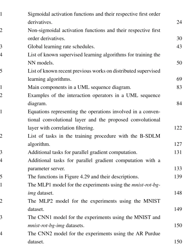
2.1 Sigmoidal activation functions and their respective first order
derivatives. 24
2.2 Non-sigmoidal activation functions and their respective first
order derivatives. 30
2.3 Global learning rate schedules. 43
2.4 List of known supervised learning algorithms for training the
NN models. 50
2.5 List of known recent previous works on distributed supervised
learning algorithms. 69
3.1 Main components in a UML sequence diagram. 83
3.2 Examples of the interaction operators in a UML sequence
diagram. 84
4.1 Equations representing the operations involved in a conven-tional convoluconven-tional layer and the proposed convoluconven-tional
layer with correlation filtering. 122
4.2 List of tasks in the training procedure with the B-SDLM
algorithm. 127
4.3 Additional tasks for parallel gradient computation. 131 4.4 Additional tasks for parallel gradient computation with a
parameter server. 133
4.5 The functions in Figure 4.29 and their descriptions. 139 5.1 The MLP1 model for the experiments using the
mnist-rot-bg-imgdataset. 148
5.2 The MLP2 model for the experiments using the MNIST
dataset. 149
5.3 The CNN1 model for the experiments using the MNIST and
mnist-rot-bg-imgdatasets. 150
5.4 The CNN2 model for the experiments using the AR Purdue
xiv
5.5 The CNN3 model for the experiments using the AR Purdue
dataset. 151
5.6 List of the hyperparameter values used in the experiments. 152 5.7 MCRs and average execution time for CNN models
composed of convolutional layers with different weight
flipping modes on the MNIST dataset. 154
5.8 MCRs and average execution time for CNN models composed of convolutional layers with different weight
flipping modes on themnist-rot-bg-imgdataset. 154 5.9 MCRs and average execution time for CNN models
composed of convolutional layers with different weight
flipping modes on the AR Purdue dataset. 154 5.10 Hyperparameters of the activation functions and the
corresponding search range during the NN training. 155 5.11 Testing MCRs of the MLPs with different activation functions
on themnist-rot-bg-imgdataset. The bolded functions denote
the proposed functions. 156
5.12 Results of the CNN models using different activation functions on MNIST dataset. The bolded functions denote
the proposed functions. 161
5.13 Hyperparameters for other activation functions and the
corresponding search range during the training. 162 5.14 Results of the CNN models using different sigmoidal
activation functions on the MNIST dataset. The bolded
function denotes the function with the proposed coefficients. 163 5.15 Results of the CNN models using different non-sigmoidal
activation functions on MNIST dataset. The bolded functions
denote the proposed functions. 165
5.16 Results of the CNN models using different activation functions on the mnist-rot-bg-img dataset. The bolded
functions denote the proposed functions. 169 5.17 Results of the CNN models using different activation
functions on the AR Purdue dataset. The bolded functions
denote the proposed functions. 170
5.18 Probability of numerical instability for the CNN models using different activation functions on the MNIST dataset. The
xv
5.19 Probability of numerical instability for the CNN models using different activation functions on themnist-rot-bg-imgdataset.
The bolded functions denote the proposed functions. 172 5.20 Probability of numerical instability for the CNN models using
different activation functions on the AR Purdue dataset. The
bolded functions denote the proposed functions. 172 6.1 Benchmarking of various learning algorithms with previous
existing works on the MNIST dataset. 175
6.2 Average execution time of a single training epoch for the MLP2 model using various learning algorithms on the
MNIST dataset. 175
6.3 Benchmarking of face recognition using the AR Purdue face
dataset. 176
6.4 CE errors and MCRs for various learning algorithms on the
MNIST dataset. 177
6.5 CE errors and MCRs for various learning algorithms on the
mnist-rot-bg-imgdataset. 178
6.6 CE errors and MCRs for various learning algorithms on the
AR Purdue dataset. 179
6.7 Average execution time per training epoch for various learning algorithms on the mnist-rot-bg-img and AR Purdue
datasets. 179
6.8 Impacts of the dataset size allocated for the Hessian estimation on the CE errors and MCRs for the MNIST
dataset. 180
6.9 Effects of different learning rate update frequencies on the CE
errors and MCRs for the MNIST dataset. 182
6.10 Effects of different mini-batch sizes on the CE errors and
MCRs for the MNIST dataset. 183
6.11 Average execution time per training epoch for various learning algorithms and their respective distributed versions based on the parameter server thread model using a single
xvi
LIST OF FIGURES
FIGURE NO. TITLE PAGE
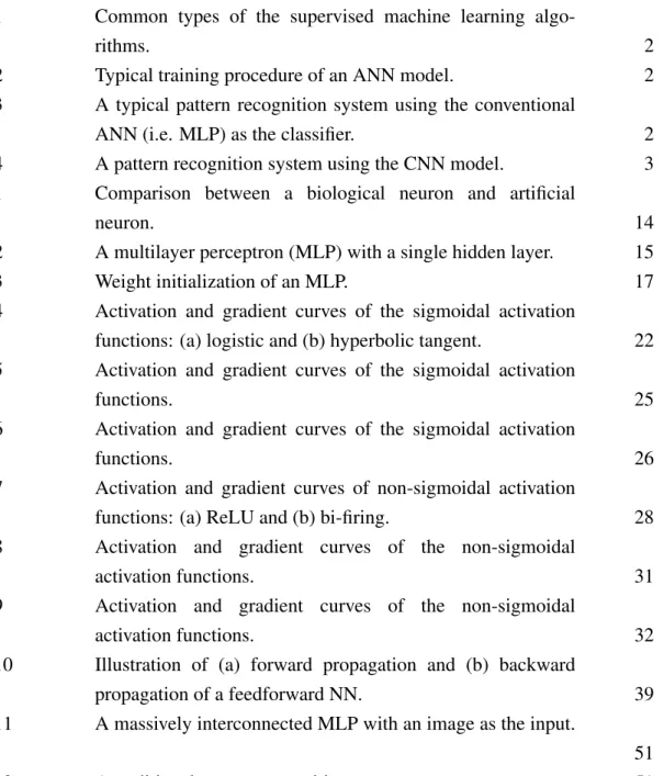
1.1 Common types of the supervised machine learning
algo-rithms. 2
1.2 Typical training procedure of an ANN model. 2
1.3 A typical pattern recognition system using the conventional
ANN (i.e. MLP) as the classifier. 2
1.4 A pattern recognition system using the CNN model. 3 2.1 Comparison between a biological neuron and artificial
neuron. 14
2.2 A multilayer perceptron (MLP) with a single hidden layer. 15
2.3 Weight initialization of an MLP. 17
2.4 Activation and gradient curves of the sigmoidal activation
functions: (a) logistic and (b) hyperbolic tangent. 22 2.5 Activation and gradient curves of the sigmoidal activation
functions. 25
2.6 Activation and gradient curves of the sigmoidal activation
functions. 26
2.7 Activation and gradient curves of non-sigmoidal activation
functions: (a) ReLU and (b) bi-firing. 28
2.8 Activation and gradient curves of the non-sigmoidal
activation functions. 31
2.9 Activation and gradient curves of the non-sigmoidal
activation functions. 32
2.10 Illustration of (a) forward propagation and (b) backward
propagation of a feedforward NN. 39
2.11 A massively interconnected MLP with an image as the input.
51
xvii
2.13 A simple DBN architecture. Pre-training is performed by training the first RBM, fixing the weightsW(0), then continue with the second RBM and repeat until all the weights are
pre-trained. 53
2.14 A four-staged neocognitron model. 55
2.15 The LeNet-5 CNN architecture. 56
2.16 Types of parallelism in distributed ML: (a) model parallelism, (b) data parallelism, and (c) combination of model and data
parallelisms. 64
2.17 Parameter server approach in the DistBelief software
framework. 65
3.1 Phases or layers of implementing an algorithm in software or
hardware for parallel computations. 78
3.2 Representations of data dependencies among the algorithm tasks: (a) dependence graph, (b) DAG, (c) DCG, and (d)
adjacency matrix. 79
3.3 Examples of different algorithm types: (a) SA, (b) PA, (c)
SPA, (d) NSPA, and (e) RIA. 80
3.4 Types of diagrams as defined in the UML specification. 81 3.5 Multiprocessor systems: (a) shared-memory with a single
system bus, (b) shared-memory with an interconnected
network, and (c) distributed-memory. 86
3.6 Common thread models: (a) manager/worker, (b) peer, and
(c) pipeline. 87
4.1 Forward propagation of a convolutional layer. 90 4.2 Forward propagation of an output neuron in a convolutional
layer. 91
4.3 Conventional connection schemes: (a) full, (b) partial, (c)
binary, and (d) Toeplitz. 92
4.4 Evolvable connection schemes: (a) dropout and (b) DropConnect. The cross denotes disabled neuron(s) or
connection(s). 93
4.5 Forward propagation of a pooling layer. 94
4.6 Forward propagation of an output neuron in a pooling layer. 95 4.7 A set of convolutional and pooling layers (above) and the
corresponding fused convolutional-pooling layer. 96 4.8 Forward propagation of a fully-connected layer. 97
xviii
4.10 Convolutions versus cross-correlations: (a) the original kernel, (b) convolution with the flipped kernel, and (c)
cross-correlation with the original kernel. 99
4.11 Activation and gradient curves of proposed activation
functions: (a) bounded ReLU and (b) leaky bounded ReLU. 100 4.12 Activation and gradient curves of the proposed bounded
bi-firing activation function. 102
4.13 Activation and gradient curves of the hyperbolic tangent
function with different sets of coefficients. 103 4.14 First order backward propagation of an output neuron in a
fully-connected layer. 105
4.15 First order backward propagation of an output neuron in a
convolutional layer. 106
4.16 First order backward propagation of an output neuron in a
pooling layer. 108
4.17 Directed cyclic graph (DCG) of the B-SDLM algorithm. 128 4.18 DAGs of the initialization stage in the B-SDLM algorithm. 129 4.19 DCG of Hessian estimation stage in B-SDLM algorithm. 129 4.20 DCG of Hessian estimation stage with (a) a model replica per
data sample or (b) a model replica per data batch. 130 4.21 DCG of the training stage in the B-SDLM algorithm. 131 4.22 DCG of the incomplete asynchronous training stage in the
B-SDLM algorithm. 132
4.23 DCG of the asynchronous training stage with a centralized
parameter memory storage. 132
4.24 (a) Diagram of a centralized parameter memory storage; and (b) DAG of the weight update operation in a parameter server.
133 4.25 DCG of the asynchronous training stage with a parameter
server. 134
4.26 DCG of the testing stage in the B-SDLM algorithm. 134 4.27 DCG of testing stage with (a) a model replica per data sample
or (b) a model replica per data batch. 135
4.28 DCG of the proposed distributed B-SDLM algorithm. 136 4.29 Sequence diagram of the proposed distributed B-SDLM
learning algorithm. 137
4.30 Critical sections of the sequence diagram in Figure 4.29 that
xix
4.31 The parameter server thread model for the (a) Pthreads and
(b) MPICH implementations. 141
4.32 Writing process on the shared memory in the Pthreads implementation: (a) replacing the data with new values, or
(b) accumulating values to the data. 142
4.33 Writing process on the shared memory in the Pthreads implementation using the pthread_mutex_trylock()
routine. 142
4.34 Writing process on the remote memory in the MPICH implementation: (a) replacing the data with new values, or
(b) accumulating values to the data. 143
4.35 Reading process of the shared memory in the Pthreads implementation by using (a)pthread_mutex_lock()or
(b)pthread_mutex_trylock(). 143 4.36 Reading process on the remote memory in the MPICH
implementation. 143
5.1 Examples of the MNIST handwritten digit images. 146 5.2 Examples of the handwritten digit images in the
mnist-rot-bg-imgdatabase. 147
5.3 The face images of a single subject in the AR Purdue face
database. 147
5.4 The CNN1 model for handwritten digit classification using
the MNIST andmnist-rot-bg-imgdatasets. 149 5.5 Training efficiencies of the CNNs with the relu and brelu
functions: (a) training losses and (b) testing MCRs using the MSE loss function; and (c) training losses and (d) testing
MCRs using the CE loss function. 158
5.6 Training efficiencies of the CNNs with the lrelu and blrelu functions: (a) training losses and (b) testing MCRs using the MSE loss function; and (c) training losses and (d) testing
MCRs using the CE loss function. 159
5.7 Training efficiencies of the CNNs with the bifire and bbifire functions: (a) training losses and (b) testing MCRs using the MSE loss function; and (c) training losses and (d) testing
MCRs using the CE loss function. 160
5.8 Training efficiencies of the CNNs with thetanhfunction with different sets of coefficient values: (a) training losses and (b) testing MCRs using the MSE loss function; and (c) training
xx
5.9 Average execution time of a single training epoch for CNN
models using different activation functions. 168 6.1 (a) Training CE errors and (b) testing MCRs for various
learning algorithms on the MNIST dataset. 177 6.2 Average execution time of a single training epoch for various
learning algorithms on the MNIST dataset. 178 6.3 (a) Training CE errors and (b) testing MCRs using different
portions of the MNIST training set for the Hessian estimation
on the MNIST dataset. 180
6.4 Average execution time of a single training epoch for different
sizes of Hessian set on the MNIST dataset. 181 6.5 (a) Training CE errors and (b) testing MCRs for different
learning rate update frequencies on the MNIST dataset. 182 6.6 (a) Training CE errors and (b) testing MCRs using different
mini-batch sizes on the MNIST dataset. 183
6.7 Testing MCRs for various distributed learning algorithms based on the parameter server thread model on (a) MNIST
and (b)mnist-rot-bg-imgdatasets. 185
6.8 CPU utilization during the training process in the Pthreads
implementation. 187
6.9 Average execution time of a single training epoch for various distributed learning algorithms based on the parameter server thread model on (a) MNIST and (b) mnist-rot-bg-img
datasets. 187
6.10 Parallelism efficiency for the proposed distributed B-SDLM learning algorithm based on the parameter server thread
model on (a) MNIST and (b)mnist-rot-bg-imgdatasets. 189 6.11 Time taken to reach a fixed classification accuracy on the
MNIST dataset for various distributed learning algorithms based on parameter server thread model: (a) 99.9% on
training set, and (b)98%on testing set. 190 6.12 Time taken to reach a fixed classification accuracy on
the mnist-rot-bg-img dataset for various distributed learning algorithms based on parameter server thread model: : (a)86%
on training set, and (b)75%on testing set. 190 6.13 (a) Testing MCRs and (b) average execution time of a single
training epoch for various distributed learning algorithms based on peer worker thread model on the MNIST dataset.
xxi
6.14 Parallelism efficiency for the proposed distributed B-SDLM learning algorithm on the MNIST dataset: (a) peer worker thread model; and (b) comparison between parameter server
and peer worker thread models. 192
6.15 Time taken to reach a fixed classification accuracy on the MNIST dataset for various distributed learning algorithms based on peer worker thread model: (a) 99%on training set,
and (b)98%on testing set. 193
6.16 Time taken to reach a fixed classification accuracy on the MNIST dataset for the proposed distributed B-SDLM learning algorithm based on different thread models: (a)99%
on training set, and (b)98%on testing set. 193 6.17 Average execution time per training epoch for (a) Pthreads
and MPICH implementations in stochastic learning mode; and (b) MPICH implementation with different mini-batch
sizes. 194
6.18 Network congestion issue of the MPICH implementation when running in the stochastic learning mode (i.e. batch size
= 1). 195
6.19 Time taken to reach a certain (a) loss value and (b) classification accuracy on the MNIST dataset when training
with batch size = 16 in the MPICH implementation. 196 F.1 Directed cyclic graph (DCG) of the distributed B-SDLM
algorithm with a centralized parameter memory storage. 245 F.2 Sequence diagram of the distributed B-SDLM algorithm
with a centralized parameter memory storage (including the
critical sections). 246
F.3 The peer worker thread model for the Pthreads
xxii
LIST OF ABBREVIATIONS
A-SGD – Asynchronous Stochastic Gradient Descent AAPNet – Autoassociative Pyramidal Neural Network AdaGrad – Adaptive Subgradient
ANN – Artificial Neural Network
API – Application Programming Interface ASIC – Application-Specific Integrated Circuit ASM – Algorithmic State Machine
B-SDLM – Bounded Stochastic Diagonal Levenberg-Marquardt BFGS – Broyden-Fletcher-Goldfarb-Shanno
BGD – Batch Gradient Descent
BP – Backpropagation
BRAIN – Brain Research through Advancing Innovative Neurotechnologies
CD – Contrastive Divergence
CDBN – Convolutional Deep Belief Network
CE – Cross-Entropy
CNN – Convolutional Neural Network ConvNet – Convolutional Network
COTS – Commodity Off-The-Shelf CPU – Central Processing Unit
CUDA – Compute Unified Device Architecture DAG – Directed Acyclic Graph
DARPA – Defense Advanced Research Projects Agency
xxiii
DCG – Directed Cyclic Graph
DeSTIN – Deep SpatioTemporal Inference Network
DG – Directed Graph
DL – Deep Learning
DLP – Data-Level Parallelism
DNN – Deep Neural Network
DSN – Deep Stacking Network
EER – Equal Error Rate
EMSO-CD – Efficient Mini-batch for Stochastic Optimization - Coordinate Descent
EMSO-GD – Efficient Mini-batch for Stochastic Optimization - Gradient Descent
FPGA – Field Programmable Gate Array
GA – Genetic Algorithm
GD – Gradient Descent
GN – Gauss-Newton
GNU – GNU’s Not Unix
GPU – Graphics Processing Unit GUI – Graphical User Interface
HCNN – Hybrid Convolutional Neural Network HDL – Hardware Description Language HPC – High Performance Computing HTM – Hierarchical Temporal Memory
I/O – Input/Output
IEEE – Institute of Electrical and Electronics Engineers ILP – Instruction-Level Parallelism
IPC – Inter-process Communication
L-BFGS – Limited-memory Broyden-Fletcher-Goldfarb-Shanno L-SDLM – Layer-specific Stochastic Diagonal Levenberg-Marquardt
xxiv
LIPNet – Lateral Inhibition Pyramidal Neural Network LMA – Levenberg-Marquardt Algorithm
LTS – Long Term Support
MATLAB – Matrix Laboratory
MCDNN – Multi-Column Deep Neural Network MCR – Misclassification Error Rate
MIMD – Multiple Instruction Multiple Data MISD – Multiple Instruction Single Data
ML – Machine Learning
MLP – Multilayer Perceptron
MNIST – Mixed National Institute of Standards and Technology
MP – Message Passing
MPI – Message Passing Interface
MPICH – Message Passing Interface Chameleon
MPF – MaxPoolingFragment
MSE – Mean Squared Error
NaN – Not a Number
NIN – Network in Network
NN – Neural Network
NSPA – Non Serial-Parallel Algorithm NUMA – Nonuniform Memory Access OOP – Object Oriented Programming OpenMP – Open Multi-Processing
OS – Operating System
PA – Parallel Algorithm
PLP – Process-Level Parallelism
POSIX – Portable Operating System Interface PSGD – Parallel Stochastic Gradient Descent
PWL – Piecewise Linear
xxv
PyraNet – Pyramidal Neural Network
RAM – Random Access Memory
RBF – Radial Basis Function
RBM – Restricted Boltzmann Machine ReLU – Rectified Linear Unit
RIA – Regular Iterative Algorithm
RMA – Remote Memory Access
Rprop – Resilient Propagation RTL – Register-Transfer Level
SA – Serial Algorithm
SCNN – Similarity Convolutional Neural Network SDLM – Stochastic Diagonal Levenberg-Marquardt SGD – Stochastic Gradient Descent
SICoNNet – Shunting Inhibitory Convolutional Neural Network SIMD – Single Instruction Multiple Data
SISD – Single Instruction Single Data SPA – Serial-Parallel Algorithm
SSE – Sum of Squared Errors
SVM – Support Vector Machine TLP – Thread-Level Parallelism
UAP – Universal Approximation Property UAT – Universal Approximation Theorem
UMA – Uniform Memory Access
UML – Unified Modeling Language
UNIX – Uniplexed Information Computing System
VHDL – Very High Speed Integrated Circuit Hardware Description Language
vSGD – Variance-based Stochastic Gradient Descent
xxvi
LIST OF SYMBOLS
(xj)m – jthvalue ofmthvector x0j
m – j
thvalue ofmthnormalized vector
(xmax)m – Maximum value ofm
thvector
(xmin)m – Minimum value ofmthvector xdmax – Desired maximum value ofm
th vector xdmin – Desired minimum value ofm
th vector
(µx)m – Mean ofmthvector
(σx)m – Standard deviation ofmthvector
M – Total training samples
MB – Total samples of a mini-batch
MH – Total samples for Hessian estimation MT – Total testing samples
U[a, b] – Uniform distribution with lower boundaryaand upper boundaryb
N(µ, σ2) – Normal distribution with meanµand standard deviationσ
b c – Floor function
f( ) – Activation function
avg( ) – Average function exp ( ) – Exponential function
f lip( ) – Flipping function
max ( ) – Maximum function min ( ) – Minimum function
PU – Upper boundary of an activation function PL – Lower boundary of an activation function
xxvii
N(l) – Total neurons (or feature maps) in layerl R(l) – Feature map’s height in layerl
C(l) – Feature map’s width in layerl
Kx(l) – Kernel’s height in layerl Ky(l) – Kernel’s width in layerl
Sx(l) – Vertical step size for convolutions in layerl Sy(l) – Horizontal step size for convolutions in layerl
Mi(l−1) – R(l−1)×C(l−1) matrix that contains indices of all activated neurons fromithfeature map in layer(l−1)
Wc – Current set of weights Wopt – Optimal set of weights
Wt – Set of weights at thetthiteration
Wthres – Threshold value of the weights
4Wt – Weight update step sizes attthiteration
Wji(l) – Weight betweenjthneuron in layerlandithneuron in layer
(l−1)
Wji(l)(u, v) – Weight(u, v)of the kernel betweenjthfeature map in layerl
andithfeature map in layer(l−1) f
Wji(l)(u, v) – Weight(u, v)of the flipped kernel betweenjthfeature map in layerlandithfeature map in layer(l−1)
Bj(l) – Bias ofjthneuron in layerl
Xj(l) – Partial summation ofjthneuron in layerl
Xj(l)(x, y) – Partial summation of neuron(x, y)atjthfeature map in layerl Yj(l) – Output ofjthneuron in layerl
Yj(l)(x, y) – Output of neuron(x, y)atjthfeature map in layerl
Yj(0)
m –
jthvalue ofmthsample (input layer)
Yj(L)
m – Output of
jthneuron in output layerLformthsample
(dj)m – Desired (target) value ofjthneuron in output layerLformth
sample
p(jL)
m – Output probability of
jth neuron in output layerLformth
xxviii
Cm – Class assigned tomthsample E – Error or loss function
Em – Error formthsample
(ESSE)m – Sum squared error formthsample
(EM SE)m – Mean squared error formthsample
(ECE)m – Cross-entropy error formthsample
(EW D)m – Error with weight decay formthsample
– Desired loss value
tmax – Maximum training epochs
tupdt – Total epochs before the learning rate update dE(W)
dW – First derivatives ofEwith respect to the weightsW ∂Em
∂Wji(l) – First derivative ofEwith respect toW
(l)
ji formthsample H(W) – Second derivatives (Hessian) matrix of the weightsW
d2E(W)
dW2 – Second derivatives ofEwith respect to the weightsW
∂2E
m
∂Wji(l)2 – Second derivative ofEwith respect toW
(l) ji formthsample ∂2E ∂Wji(l)2 – Running average of ∂2E ∂Wji(l)2 ∂2E ∂Wji(l)2 – Average of ∂2E ∂Wji(l)2
η – Global learning rate
ηopt – Optimal global learning rate η(l) – Global learning rate for layerl
ηW(l)
ji
– Learning rate for weightWji(l) α – Weight regularization constant
β – Momentum rate
γ – Memory constant
µ – Regularization parameter
xxix
LIST OF APPENDICES
APPENDIX TITLE PAGE
A Publications 227
B Fan-in and Fan-out Calculations for Different Types of
Neuron Layers 229
C First Order Backward Propagations for Different Types of
Neuron Layers 232
D Propositions for the Proposed Activation Functions based on
the UAT 237
E Derivation of Better Coefficient Values for the Scaled
Hyperbolic Tangent Function 242
F Distributed B-SDLM Learning Algorithm based on the Peer
Worker Approach 244
CHAPTER 1
INTRODUCTION
1.1 Artificial Neural Networks
An artificial neural network (ANN) is a biologically inspired mathematical model that consists of a group of artificial neurons. A neuron (commonly known as perceptron [1]) is a single processing entity comprised of some functions (partial summation by default), a bias (determines threshold), and an activation function (provides nonlinearity behavior [2]) which is usually a sigmoidal function. Such neurons are interconnected among each other by the weights (define the connection strengths among these neurons), and multiple layers of these neurons form a powerful hierarchical structure commonly known as the multilayer perceptron (MLP).
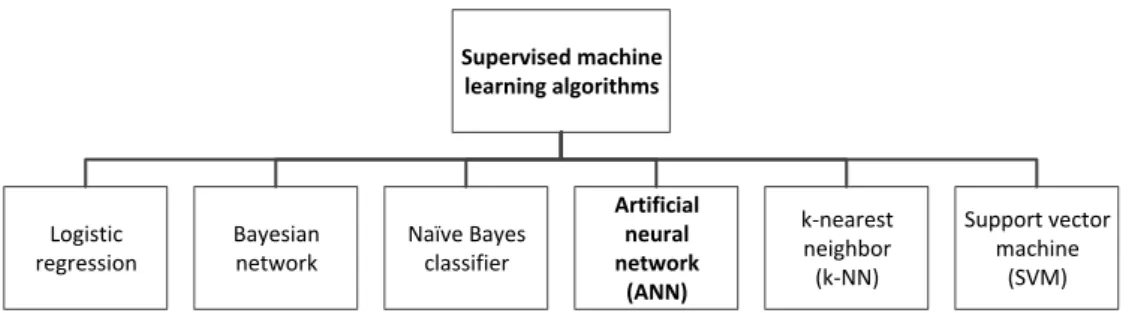
ANNs possess the ability to learn from data, and the process of learning is known as the training process. Typical ANNs are usually trained based on the labels assigned to the data, hence are often categorized as supervised machine learning algorithms [3, 4, 5] (as depicted in Figure 1.1). A typical training procedure consists of a series of tasks (Figure 1.2), i.e. weight initialization (generates random weights as a starting point), forward propagation (propagates the inputs through the ANN to calculate the outputs), backward propagation (calculates the error gradients by propagating the errors from the output to input layers), and weight update (tunes the weights based on the error gradients to learn better) [6]. An input sample is typically normalized into a range that is suitable to be processed by the ANN. Classification is usually performed by determining the output neuron that produces the maximum value (i.e. winner-takes-all (WTA)). A loss function is essential to evaluate the learning performance of the ANN and calculate the errors to be backward propagated. A typical example is the mean squared error (MSE) loss function.
2 Supervised machine learning algorithms Artificial neural network (ANN) Support vector machine (SVM) Logistic regression Bayesian network Naïve Bayes classifier k-nearest neighbor (k-NN)
Figure 1.1: Common types of the supervised machine learning algorithms.
Input normalization Weight initialization Forward propagation Classification Loss calculation Backward propagation Weight update
Figure 1.2: Typical training procedure of an ANN model.
common learning algorithm is the gradient descent (GD) method [7], which typically operates in one of the three learning modes: updates the weights after processing all the samples once (batch mode); updates them after processing a single sample (stochastic); or a combination of both (mini-batch mode). A learning rate mainly dictates the update step sizes for these weights, and is usually manually tuned (i.e. a hyperparameter).
ANNs have been successfully applied in solving various classification, prediction, and control problems due to its powerful learning ability. For a given problem, a feature extractor is usually designed to generate a compact and meaningful feature for an input sample, which is then processed by the ANN to produce the result (as shown in Figure 1.3). They are suitable for any complex problems that have no definite algorithmic solutions or are too difficult to be expressed algorithmically.
Raw input Preprocessing module Trainable classifier (MLP) Result Feature extraction module Feature vector Dimensionality reduction module Compressed input Preprocessed input
Figure 1.3: A typical pattern recognition system using the conventional ANN (i.e. MLP) as the classifier.
However, conventional ANNs (i.e. MLPs) do have many drawbacks and limitations. A larger ANN model can present a better solution, yet is often harder and slower to be trained due to its massively interconnected and rigid structure. Such structure is very compute-intensive, and often leads to the overfitting problem during the learning [8], where the model tends to memorize the training samples instead of
3
generalizing from them and be able to classify the unseen samples correctly.
Since a conventional ANN is unable to handle the raw input patterns, re-design of the complete system is required whenever the problem domain changes [9]. Also, typical ANNs have a planar structure that ignores the input topology for any given problem [10], hence can perform poorly on the distorted samples due to having only little or no invariance to such input distortions.
1.2 Convolutional Neural Networks
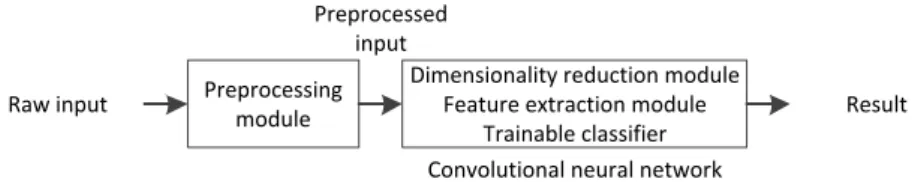
Convolutional neural networks (CNNs) are a variant of the ANNs that attempts to alleviate the aforementioned problems with the conventional ANN models [9, 11]. Inspired by the animal’s visual system [12], the CNN differs from the conventional ANNs by incorporating the feature extraction, dimensionality reduction, and classification into a single hierarchical model (see Figure 1.4). The weight sharing concept is also implemented in the CNN model that breaks the rigid structure of the conventional ANNs [9], allowing it to achieve better generalization performance, especially when dealing with the multi-dimensional computer vision problems.
Raw input Preprocessing
module Result Dimensionality reduction module
Feature extraction module Trainable classifier Preprocessed
input
Convolutional neural network
Figure 1.4: A pattern recognition system using the CNN model.
A typical CNN model consists of a few types of neuron layers: convolutional layers, pooling layers, fully-connected layers, and softmax layer. The convolutional layers perform convolutions to extract features from the inputs and produce the feature maps. A pooling layer reduces the dimension of a feature map while preserving the spatial locality of the features in the feature map. Fully-connected layers work similar to the MLP that performs classification and regression. A softmax layer calculates the probability of the class for an input sample, which is often used in conjunction with the cross-entropy (CE) loss function. Training a CNN model is similar to the conventional ANNs, where similar training procedures and learning algorithms are usually applied to both model types [9].
4
CNNs have shown great success in solving various kinds of visual pattern recognition problems, which include classifications, verifications, detections, tracking, and many more [13, 14, 15, 16]. Motivated by the superiority of the CNN in the computer vision applications, CNNs have become a very active research area in both academia and industries. For instance, many giant companies such as Facebook, Google, and Microsoft have released various products and services with CNNs as the underlying algorithm [17, 18, 19, 20]. More complex and powerful CNN models have been proposed to deal with the real-world complex problems, which motivates the research direction towards the deep learning and distributed machine learning.
1.3 Deep Learning and Distributed Machine Learning
Deep learning (DL) is a branch of machine learning (ML) algorithms that learn deeper abstractions of meaningful features by constructing a hierarchical model with multiple processing layers that perform nonlinear transformations [14]. The idea is based on the complex and hierarchical computations involved in a biological brain [21]. A typical example of the DL model is deep neural network (DNN). Notwithstanding the greater learning ability of the DL models that tend to achieve superior classification performance, training such complex models is extremely computationally expensive and difficult [22]. The problem becomes even more apparent when dealing with large-scale databases with tens of thousands of samples or more, and running on a single processor sequentially as in the traditional implementations [22]. This motivates the development of distributed ML techniques that aim to accelerate the training process through parallelism.
The concept of distributed ML is to distribute the training process to multiple processing units or machines in a parallel or distributed computing platform [19]. These computing platforms can be a multi-core central processing unit (CPU) system [23], a single system with multiple graphics processing units (GPUs) [24], or even a large-scale computer cluster [19]. Various fine-grained optimizations are performed on different computing platforms to achieve scalable parallelism speedup [19, 25, 26, 27]. This thesis generally denotes these platforms as parallel computing platforms for simplicity purposes.
Distributed versions of the conventional learning algorithms have been developed to train the DL models in the distributed ML environment. These
5
algorithms are usually derived from the stochastic gradient descent (SGD) that support asynchronous weight updates, and most of them are first order learning algorithms [19, 20, 25, 28, 29, 30, 31]. All these advancements make the training of a DL model possible, which often leads to the state-of-the-art performances in various pattern recognition problems.
1.4 Problem Statement
CNNs have shown great potentials in the computer vision problems as reported in current literature [13, 14, 15, 16]. Still, there are several outstanding issues with the modeling of CNN and the learning algorithm. Computational efficiency and effective learning convergence of the CNN model are the primary goals of this thesis.
A typical CNN model is a hierarchical structure consisting several neuron layers. Convolutional layer constitutes a great proportion of the computational complexity in a CNN model [29]. Forward and backward propagations through a convolutional layer require flipping of the kernel weights due to the spatial convolution operations [32, 33]. This can be performed by exchanging values between the memory locations, or manipulating the memory addressing during the convolutions. Either method slows down the computational time of a CNN model. More importantly, the effect of the weight flipping on the generalization performance of the CNN remains an open question, which is one of the main focuses in this thesis.
In addition, there has been confusion between using either discrete convolutions or cross-correlations in the convolutional layers by analyzing a wide range of previous works. Some have reported to perform convolutions, but instead using cross-correlation operations as indicated by their mathematical representations of a convolutional layer [34, 35, 36, 37, 38].
As a mathematical model that provides nonlinearity to ANNs [2, 39], the impacts of an activation function on the generalization performance and training stability of an NN model are often ignored. There is a lack of consensus on how to select a good activation function for an NN, and a specific activation function may not be suitable for all applications. This is especially true for problem domains where the numerical boundaries of the inputs and outputs are the main considerations.
6
Also, their effect on the generalization performance of DNN models remains an open question, since most comparative studies on the activation functions were only performed on simple and shallow MLP models [40, 41, 42]. Some previous works evaluated on the DNN models, yet covered a few common activation functions only [43, 44]. As different activation functions have different input and output characteristics, the effect of using different loss functions during a training process on the learning performance of a DNN model is yet to be determined.
An NN training process is heavily dependent on the choice of the activation function. As most supervised learning algorithms are based on the backward propagation of the error gradients, the tendency at which an activation function saturates is one of the main concerns during the backward propagation. This is because the saturation problem can lead to inefficient propagation of the error gradients (i.e. gradient diffusion problem), which can result in poor learning convergence [45, 46]. Common examples include the logistic and hyperbolic tangent activation functions [10].
Some modified functions such as scaled hyperbolic tangent with specific coefficients attempt to alleviate this problem [9]. However, these coefficients do not satisfy the characteristics that are claimed to improve the network convergence. Some non-sigmoidal functions can propagate gradients well, but numerical instability can occur due to unbounded output values [46]. Also, since an activation function is applied to the outputs of all neurons in most cases, its computational complexity will contribute heavily to the overall execution time of an NN model.
Most research works on the activation functions are focused on the complexity of the nonlinearity that an activation function can provide [2], how well it can propagate errors [46], or how fast it can be executed [47], but often neglect its impact on the overall training stability due to the numerical stability. The numerical stability of a training process is largely dependent on the input and output boundaries of the activation function as well as the numerical representation of the physical computing machine. Larger boundary values allow for more efficient propagation of neurons’ values [46], but with higher risk of getting into the numerical overflow problem, which causes unstable outputs in a trained NN model. This should be taken into considerations as well when designing a suitable activation function for an NN model.
Regardless of how well the learning capacity of a model is, the learning performance is still highly dependent on the effectiveness of its learning algorithm.
7
A learning algorithm defines how a trainable model can make use of the underlying information within the data, and learn from its statistics.
Convergence rate has been an important criterion in choosing a suitable learning algorithm. First order methods are widely used in NN training [7], yet suffer from slow convergence and higher chance of reaching poor local minima. Some previous works have shown the benefits of having learning rate annealing on the convergence speed in NN training [48], yet with the expense of introducing more hyperparameters. An adaptive learning rate schedule should be hyperparameter free to reduce the effort of manually tuning these variables as little as possible.
Second order learning algorithms generally converge faster than first order methods due to the utilization of both gradient and curvature information of a problem [49]. Despite their fast convergence rate, they are impractical in solving DL problems due to being very computationally expensive [49]. Most second order learning algorithms only support batch learning mode [50, 51], which are less effective in propagating the error gradients.
Some second order stochastic learning algorithms such as the stochastic diagonal Levenberg-Marquardt (SDLM) have been proposed [9], yet these algorithms usually contain more hyperparameters than conventional first order methods. This can result in the hyperparameter overfitting problem [52], in which there are endless ways of configuring the learning algorithm, and this may end up selecting a combination of values that outperforms others purely by chance. More importantly, this will drastically increase the difficulty of finding a good solution, as most efforts are devoted to selecting good hyperparameter values by means of trial and error, which is more of an art than science. Moreover, some learning algorithms are hyperparameter sensitive, as choosing an inappropriate combination of values can even cause numerical instability [52]. It is likely that the reluctant adoption of second order methods in DL is related to these outstanding issues.
In general, stochastic learning algorithms reach convergence faster than batch algorithms due to the noisy weight updates that increase the tendency of escaping from local minima [49]. On the contrary, a batch algorithm can be easily parallelized to support parallel computation that results in faster training time. Most state-of-the-art works have been utilizing the mini-batch version of SGD to train DNNs [19, 25, 28]. How a stochastic second order learning algorithm performs when running in mini-batch learning mode remains an open question.
8
The concept of distributed ML attempts to solve the problem of training larger and deeper NN models (deep learning) on large-scale datasets (big data). Most existing works focused on the performance speedup gained from fine-grained parallelism, which includes optimizations for different computing platforms, various implementation approaches, and techniques to reduce the communication bandwidth [19, 25, 26, 27]. However, these works rarely discussed on the importance of an efficient and effective distributed learning algorithm.
Common distributed learning algorithms are usually derived from conventional first order methods (particularly SGD) [19, 25, 28]. However, first order learning algorithms are known to be inefficient because of their slow convergence, and they are also prone to other learning issues [45, 49]. Second order algorithms, such as Levenberg-Marquardt algorithm (LMA), use the Hessian matrix to perform better estimation of both step sizes and directions, so that they can converge much faster than first order algorithms [49]. Research reported in [19, 53, 54] have applied second order learning algorithms for distributed learning in batch learning mode; however, in most cases, they did not outperform the distributed SGD.
Some distributed learning algorithms, like those proposed in [19] and [55] are effective in training deep models, but they are too computationally expensive due to re-evaluation of instantaneous learning rates in each training iteration. Comparisons among these algorithms in terms of computational time have not been clearly discussed in current literature.
Deep learning (DL), like most large-scale problems, achieves learning within reasonable computational time through parallel and distributed computing. Most existing works focus on the implementation issues of learning algorithms on parallel computing platforms; but are limited in the discussions of the algorithmic mapping process [30, 56, 57]. In [19] and [29], this mapping process is discussed, but rather briefly, hence rather inadequate to lead to good results. The design methodology of mapping a learning algorithm for parallel computation serves an important role in deriving a learning algorithm that is suitable for distributed computing environment to achieve the best possible performance speedup.
9
1.5 Objectives
The primary objective of this thesis is to improve on the existing CNN models, to propose an effective learning algorithm to train the CNNs, and to map it into a distributed machine learning environment to achieve fast parallelism speedup. In detail, the objectives of this thesis are:
1. To propose an efficient convolutional neural network (CNN) model that consists of the convolutional layers with correlation filtering and bounded activation functions for faster computation, improved generalization performance and better training stability.
2. To develop an effective stochastic second order learning algorithm, i.e. bounded stochastic diagonal Levenberg-Marquardt (B-SDLM) that converges faster, alleviates the hyperparameter overfitting problem, and is computationally efficient.
3. To propose a distributed second order learning algorithm that can converge faster and better than the common distributed first order learning algorithms, and present a systematic methodology of mapping the proposed learning algorithm for parallel computation.
1.6 Scope of Work
The work in this thesis uses a variety combination of tools and software libraries to assist in modeling, design and implementation of the proposed algorithms. The approaches, software tools, performance measures, and case studies are summarized as follows:
• The development of the proposed learning algorithm is targeted for the supervised training mode on the NN models. The computation of the error gradients is based on the standard backpropagation (BP) algorithm.
• All the proposed algorithms (including the NN models) are developed in C/C++ programming languages. Pthreads and MPICH libraries are applied for two different parallel computing platforms.
• The code compilations are performed by the GNU G++ native compiler in the Ubuntu Linux14.04 64-bit LTS OS, except for the MPICH implementation that
10
requires MPI C++ as the compiler. All the compiler optimizations are turned on (level 3) for maximum performance. Real-valued data is represented by the single-precision floating data type throughout the experiments.
• All the single and multi-threaded software programs are executed on a computer with an overclocked 4.5 GHz Intel Core i7 4790K processor and 4GB RAM. As for the MPICH implementation, the MPI program runs on a simple Beowulf computer cluster consisting of 4 identical computers as described previously, which are all connected with a 8-port Gigabit network switch.
• The experimental results and analysis are illustrated using MATLAB in the output forms of graphs and bar charts. It is also used for minimal preprocessing of the datasets (data format conversion).
• The viability of the resulting CNN models and learning algorithms is demonstrated with the performance analysis of the complex, real world case studies. The case studies used to verify and analyze the performances of the proposed CNN models and learning algorithms are limited to the following problems:
1. Basic handwritten digit classification using the MNIST database [9]; 2. Complex handwritten digit classification using the mnist-rot-bg-img
database [58]; and
3. Face recognition using the AR Purdue database [59].
• All the case studies applied in this thesis are multinomial classification problems. Common biometric performance measures such as the equal error rate (EER) are irrelevant in this thesis. Instead, the performance of an NN model is evaluated based on its classification accuracy and misclassification error rate (MCR).
1.7 Contributions
The CNN model presented in this thesis has an efficient structure over the existing works. A fast second order learning algorithm is proposed to train the CNN model effectively while performing better than most supervised learning algorithm. In addition, the distributed version of the proposed learning algorithm is developed to achieve scalable parallelism speedup when training the CNN models. In summary, the main contributions of this thesis are:
11
• This work demonstrates the effectiveness of cross-correlation filtering in a convolutional layer of the CNN model compared to the conventional convolution filtering to achieve faster execution speed and better learning performance. • Three novel bounded activation functions are proposed in this thesis, namely
bounded rectified linear unit (ReLU), bounded leaky ReLU, and bounded bi-firing functions. These activation functions improve the generalization performance of an NN model and reduce the numerical instability during the training process.
• This thesis proposes a new set of coefficient values for the scaled hyperbolic tangent activation function based on the desired properties of an activation function as reported in [9], which performs better than the function in the previous work in terms of the classification accuracy.
• A novel second order stochastic learning algorithm, i.e. B-SDLM is proposed to train the NN models. It has minimal computational overhead than SGD due to the simpler Hessian estimation, while achieving significantly better convergence rate than similar existing works. The learning algorithm contains only a single hyperparameter that alleviates the hyperparameter overfitting problem, while ensuring the training stability due to the boundary condition on the learning rates. This work is also among the first attempts to run the stochastic second order learning algorithm (i.e. the B-SDLM) in the mini-batch learning mode for better parallelism.
• A distributed version of the B-SDLM learning algorithm is developed to train the CNN models on the parallel computing platform. The proposed distributed B-SDLM learning algorithm performs better than the conventional asynchronous SGD algorithm on the same parallel computing platform, which demonstrates its superiority over the distributed first order learning algorithms in the previous works.
• This thesis presents a systematic methodology of mapping a learning algorithm into the deployment on parallel computing platforms. The learning algorithm is parallelized based on the parameter server thread model. To our knowledge, this is among the first successful attempts of mapping a stochastic second order learning algorithm for parallel computation. The experimental results have shown the viability of running a second order learning algorithm in the distributed learning environment while gaining fair parallelism speedup.
12
1.8 Thesis Organization
This thesis is organized into seven chapters. Chapter 2 describes the background theory of the ANN, deep learning (including the CNN model), and distributed machine learning. It also covers the literature review of the related previous works.
Chapter 3 presents the methodology for the research work done in this thesis. This includes the approach taken to conduct the research, software libraries and tools used, as well as the methodology of mapping the algorithms towards the parallel computing platforms.
Chapter 4 covers the fundamentals of the CNN model, and proposes a better convolutional layer and activation functions for an efficient CNN model. The training procedure with the proposed learning algorithm for the NN models is presented here. This chapter also presents the mapping process of the proposed learning algorithm into the distributed ML environment to achieve fast parallelism speedup. The coding and implementation details are also described here.
Chapter 5 presents the experimental design, results and analysis of the proposed CNN models in this thesis. These include the performance evaluation of the convolutional layer with correlation filtering, and the comparative analysis of various activation functions (including the proposed functions).
Chapter 6 presents the experimental results and analysis of the learning algorithms proposed in this thesis, including the benchmarking of the learning algorithm and training speedup of the distributed learning algorithm on different parallel computing platforms. Discussions and justifications of the work are done in this chapter as well.
Chapter 7 summarizes the thesis, re-stating the contributions based on the results, and suggests directions for future research works.
REFERENCES
1. Rosenblatt, F. The Perceptron: A Probabilistic Model for Information Storage and Organization in the Brain. Psychological Review, 1958. 65(6): 386–408.
2. Sodhi, S. S. and Chandra, P. Bi-modal Derivative Activation Function for Sigmoidal Feedforward Networks. Neurocomputing, 2014. 143: 182–196. ISSN 0925-2312. doi:10.1016/j.neucom.2014.06.007.
3. Jordan, M. I. and Mitchell, T. M. Machine Learning: Trends, Perspectives, and Prospects. Science, 2015. 349(6245): 255–260. doi:10.1126/science. aaa8415.
4. Ayodele, T. Types of Machine Learning Algorithms. INTECH Open Access Publisher. 2010.
5. Kotsiantis, S., Zaharakis, I. and Pintelas, P. Machine Learning: A Review of Classification and Combining Techniques. Artificial Intelligence Review, 2006. 26(3): 159–190. ISSN 0269-2821. doi:10.1007/s10462-007-9052-3. 6. Rumelhart, D. E., Hinton, G. E. and Williams, R. J. Learning Internal
Representations by Error Propagation. In: Rumelhart, D. E., McClelland, J. L. and PDP Research Group, C., eds. Parallel Distributed Processing: Explorations in the Microstructure of Cognition, Vol. 1. Cambridge, MA, USA: MIT Press. 318–362. 1986. ISBN 0-262-68053-X.
7. Igel, C. and Hüsken, M. Improving the Rprop learning algorithm. Proceedings of the Second International Symposium on Neural Computation, 2000. 2000: 115–121.
8. Almási, A.-D., Wo´zniak, S., Cristea, V., Leblebici, Y. and Engbersen, T. Review of Advances in Neural Networks: Neural Design Technology Stack. Neurocomputing, 2016. 174, Part A: 31–41. ISSN 0925-2312. doi: 10.1016/j.neucom.2015.02.092.
9. Lecun, Y., Bottou, L., Bengio, Y. and Haffner, P. Gradient-based Learning Applied to Document Recognition. Proceedings of the IEEE, 1998. 86(11): 2278–2324. ISSN 0018-9219. doi:10.1109/5.726791.
208
10. Cai, M. and Liu, J. Maxout Neurons for Deep Convolutional and LSTM Neural Networks in Speech Recognition. Speech Communication, 2016. 77: 53–64. ISSN 0167-6393. doi:10.1016/j.specom.2015.12.003.
11. LeCun, Y., Boser, B., Denker, J., Henderson, D., Howard, R., Hubbard, W. and Jackel, L. Backpropagation Applied to Handwritten Zip Code Recognition. Neural Computation, 1989. 1(4): 541–551. ISSN 0899-7667. doi:10.1162/neco.1989.1.4.541.
12. Hubel, D. H. and Wiesel, T. N. Receptive Fields, Binocular Interaction and Functional Architecture in the Cat’s Visual Cortex. The Journal of Physiology, 1962. 160(1): 106–154. ISSN 1469-7793. doi:10.1113/jphysiol. 1962.sp006837.
13. Antipov, G., Berrani, S.-A. and Dugelay, J.-L. Minimalistic CNN-based Ensemble Model for Gender Prediction from Face Images. Pattern Recognition Letters, 2016. 70: 59–65. ISSN 0167-8655. doi:10.1016/j. patrec.2015.11.011.
14. Chen, Y., Yang, X., Zhong, B., Pan, S., Chen, D. and Zhang, H. CNNTracker: Online Discriminative Object Tracking via Deep Convolutional Neural Network. Applied Soft Computing, 2016. 38: 1088–1098. ISSN 1568-4946. doi:10.1016/j.asoc.2015.06.048.
15. Liu, L., Xiong, C., Zhang, H., Niu, Z., Wang, M. and Yan, S. Deep Aging Face Verification With Large Gaps.Multimedia, IEEE Transactions on, 2016. 18(1): 64–75. ISSN 1520-9210. doi:10.1109/TMM.2015.2500730.
16. Shi, B., Bai, X. and Yao, C. Script Identification in the Wild via Discriminative Convolutional Neural Network. Pattern Recognition, 2016. 52: 448–458. ISSN 0031-3203. doi:10.1016/j.patcog.2015.11.005.
17. He, K., Zhang, X., Ren, S. and Sun, J. Delving Deep into Rectifiers: Surpassing Human-Level Performance on ImageNet Classification. CoRR, 2015. abs/1502.01852.
18. Taigman, Y., Yang, M., Ranzato, M. and Wolf, L. DeepFace: Closing the Gap to Human-Level Performance in Face Verification. Computer Vision and Pattern Recognition (CVPR), 2014 IEEE Conference on. 2014. 1701–1708. doi:10.1109/CVPR.2014.220.
19. Dean, J., Corrado, G., Monga, R., Chen, K., Devin, M., Mao, M., Ranzato, M., Senior, A., Tucker, P., Yang, K., Le, Q. V. and Ng, A. Y. Large Scale Distributed Deep Networks, Curran Associates, Inc. 2012, 1223–1231. 20. Le, Q. V., Ranzato, M., Monga, R., Devin, M., Chen, K., Corrado, G.,