RVD2: An ultra-sensitive variant detection model for low-depth heterogeneous next-generation sequencing data

Worcester Polytechnic Institute

Digital WPI

Masters Theses (All Theses, All Years) Electronic Theses and Dissertations

2014-04-29

RVD2: An ultra-sensitive variant detection model

for low-depth heterogeneous next-generation

sequencing data

Yuting He

Worcester Polytechnic Institute

Follow this and additional works at:https://digitalcommons.wpi.edu/etd-theses

This thesis is brought to you for free and open access byDigital WPI. It has been accepted for inclusion in Masters Theses (All Theses, All Years) by an

Repository Citation

He, Yuting, "RVD2: An ultra-sensitive variant detection model for low-depth heterogeneous next-generation sequencing data" (2014).Masters Theses (All Theses, All Years). 499.

RVD2: An ultra-sensitive variant detection model for

low-depth heterogeneous next-generation sequencing data

by Yuting He

A Thesis

Submitted to the Faculty of the

WORCESTER POLYTECHNIC INSTITUTE In partial fulfillment of the requirements for the

Degree of Master of Science in

Biomedical Engineering by

May 2014 APPROVED:

Professor Patrick J. Flaherty, Major Thesis Advisor Professor Dirk R. Albrecht, Committee member Professor Andrew C. Trapp, Committee member

Abstract

Motivation: Next-generation sequencing technology is increasingly being used

for clinical diagnostic tests. Unlike research cell lines, clinical samples are often genomically heterogeneous due to low sample purity or the presence of genetic sub-populations. Therefore, a variant calling algorithm for calling low-frequency poly-morphisms in heterogeneous samples is needed.

Results: We present a novel variant calling algorithm that uses a hierarchical

Bayesian model to estimate allele frequency and call variants in heterogeneous sam-ples. We show that our algorithm improves upon current classifiers and has higher sensitivity and specificity over a wide range of median read depth and minor al-lele frequency. We apply our model and identify twelve mutations in the PAXP1 gene in a matched clinical breast ductal carcinoma tumor sample; two of which are loss-of-heterozygosity events.

Acknowledgements

I would like to begin by expressing my deepest gratitude to my major advisor, Professor Patrick Flaherty, for all the support and guidance from the onset of my experience at Worcester Polytechnic Institute. He has rich fund of knowledge in machine learning, statistics, bioinformatics and cancer genomics, fields I have been so much fascinated by and would like to dedicate my lifelong research to. I owe un-ending thanks to him for taking me into his lab as his first graduate student, helping me get off to an amazing project and supporting me with his sustained patience, optimism, confidence, expertise and guidance throughout this entire project. I have greatly benefited from his help in many other ways as well such as building up con-fidence, confronting personal shortcomings, fighting pressure, improving technical communication skills in order to achieve overall success in my life. He is the best advisor and most thoughtful friend I can possibly have the fortune to know in my life and I will never forget him.

I would like to thank the rest of my thesis committee: Professor Andrew Trap-p and Professor Dirk Albrecht, for their encouragement and insightful comments. Their input and assistance was vital to the completion of this project and my thesis. Special thanks to Professor Yitzhak Mendelson, who took me on-board and taught me the first research skills during my first lab rotation at WPI. His rigor-ousness in research, teaching and life keeps spurring me to pursue high standard outcomes. I have Professor Ki Chon to thank for all his group meetings I attended, which have been a valuable source of knowledge, inspiration and friendship. My appreciation also goes to Professor Marshal Rolle, who was always there offering me constructive comments and warm encouragement when I was struggling with making decisions.

cam-pus. Many thanks to Jiaojiao Li, Linglong Zhu, Fan Zhang, Yanni Wang, Hachem Saddiki, Hugo Fernando Posada Quintero, Bersain Reyes, Duy Dao, Dr. Natasa Reljin, Jeffrey Bolkhovsky, Kyra Burnett, Joshua Harvey and other friends whom I’ve had the honor of meeting and knowing. I am tremendously thankful for their company and friendship.

I have my special thanks to my boyfriend, Heng Zhao, who has been extraordi-narily considerate and supportive in the last four years. Twelve hours of jet lag and 11K kilometers apart for two years is a enormous challenge to any relationship, and I’m so grateful that he has been together with me through all the ups and downs. Finally and most importantly, my families on the other side of earth will constantly be the original force which keeps me moving forward.

Contents

1 Introduction 2

1.1 Next generation sequencing . . . 2

1.2 Mutation detection . . . 4 1.3 Graphical Model . . . 5 1.3.1 Exact Inference . . . 6 1.3.2 Sampling Inference . . . 7 1.3.3 Variational Inference . . . 8 1.4 Thesis Organization . . . 9 2 Methodology 12 2.1 Model Structure . . . 12 2.2 Sampling Inference . . . 15 2.2.1 Initialization . . . 17 2.2.2 Sampling from p(θij|rij, nij, µj, M) . . . 17 2.2.3 Sampling from p(µj|θji, Mj, µ0, M0) . . . 18 2.3 Variational Inference . . . 19

2.3.1 Evidence Lower Bound (ELBO) . . . 19

2.3.2 Factorization . . . 20

2.3.3 Variational Expectation-Maximization . . . 20

2.4.1 Posterior Distribution Test . . . 23

2.4.2 χ2 _{test for non-uniform base distribution . . . 24}

3 Data 26 3.0.3 Synthetic DNA Sequence Data . . . 26

3.0.4 HCC1187 Sequence Data . . . 28

4 Result — MCMC Inference 29 4.1 Synthetic dataset . . . 29

4.1.1 Estimated MAF for variants. . . 30

4.1.2 Performance with read depth . . . 30

4.1.3 Performance comparison with other algorithms . . . 31

4.2 HCC1187 primary ductal carcinoma sample . . . 36

4.2.1 Performance of RVD2. . . 36

4.2.2 Performance comparison with other algorithms. . . 37

5 Alternative Approaches in MCMC inference 40 5.1 Proposal distribution in Metropolis-Hasting sampling . . . 40

5.1.1 Detailed balance . . . 40

5.1.2 Obtain σj from ˆµj . . . 41

5.2 Gibbs Sampling size . . . 42

5.3 Metropolis-Hasting sampling size . . . 43

5.4 Optimal Threshold τ∗ in posterior density test . . . 44

6 Discussion and Future work 45 6.1 Discussion . . . 45

6.2 Future Work . . . 46

B Simulation Example 49

C Parameter Initialization Derivation 50

D RVD2 Estimated Parameters 52

E MCMC trace and autocorrelation analysis 55

F ROC curve with χ2 _{test 57}

G Somatic mutations posterior histogram 58

H Parameter settings for other variant calling algorithms 60

I Positions Look-up chart in HCC1187 sample 62

J Variational Inference Derivation 65

J.1 Factorization . . . 65

J.2 Writing out the ELBO . . . 65

J.3 Variational Expectation (E-step) . . . 67

J.3.1 Variational distributions . . . 67

J.3.2 E-step using Beta-Beta variational distribution . . . 70

J.3.3 E-step using Beta-Laplace variational distribution . . . 71

J.4 Optimizing Model Parameters φ={µ0, M0, M} (M-step) . . . 72

J.4.1 Optimizing µ0 . . . 72

J.4.2 Optimizing M0 . . . 73

J.4.3 Optimizing M . . . 74

List of Figures

1.1 Graphical model representation of LDA for document topic modeling. 6 2.1 RVD2 Graphical Model. . . 12 3.1 DNA sequence synthesis and sequencing flowchart. . . 27 4.1 Estimated minor allele fraction for called variants in 1.0% dilution. . 30 4.2 ROC curve varying read depth showing detection performance in

syn-thetic dataset. . . 31 4.3 Sensitivity/Specificity comparison of RVD2 with other variant calling

algorithms using synthetic sequence data. . . 33 4.4 False discovery rate comparison of RVD2 with other variant calling

algorithms using synthetic sequence data. . . 34 4.5 Matthews correlation coefficient (MCC) comparison with other

vari-ant calling algorithms. . . 35 4.6 Estimated minor allele fraction for Germline and Somatic mutations

called by RVD2 in the 44kbp PAXIP1 gene from chr7:154738059 to chr7:154782774. . . 37 4.7 Positions called by VarScan2-somatic, muTect, RVD2 and Strelka in

the 44kbp PAXIP1 gene from chr7:154738059 to chr7:154782774 for performance comparison. . . 38

5.1 Standard deviation with respect to mean in proposal distribution

Q(µ∗_j|µ(_jp))_∼N(µ(_jp), σ2

j) for Metropolis-Hasting sampling. . . 41

5.2 Histogram of µcontrol

j and µcasej to evaluate the sufficiency of Gibbs

sampling size. . . 42 5.3 Histogram ofµcontrol_j andµcase_j to evaluate the sufficiency of

Metropolis-Hasting sampling size. . . 43 5.4 An simulation example to illustrate the proposal graphical model and

generative process. . . 44 A.1 Synthetic gene sequence. . . 48 B.1 An simulation example to illustrate the proposal graphical model and

generative process. . . 49 D.1 Key parameters for RVD2 model for synthetic DNA data sets. . . 53 E.1 MCMC traces and autocorrelation evaluation plot. . . 56 F.1 ROC curve for posterior density test andχ2 _{test in synthetic dataset. 57}

G.1 Histogram of ˆµj for positions where µcase is significantly lower than

µcontrol_{. . . 58}

G.2 Histogram of ˆµj for positions where µcase is significantly higher than

Chapter 1

Introduction

1.1

Next generation sequencing

The fundamental goal of genetics is to associate genotypes with observed pheno-types. In order to observe the genotype, DNA must be sequenced. DNA sequencing technology has numerous application fields such as diagnostic, molecular biology, evolutionary biology, ecology, epidemiology and virology research.

The conventional capillary-based sequencing technology, or Sanger sequencing technology is the mainstream technology for from late 1970s till late 1990s. Next-generation sequencing(NGS) method made its debut in the mid to late 1990s [60]. The real sequencing revolution came along with the sequencing-by-synthesis tech-nology from 454 Life Sciences5 and the multiplex polony sequencing protocol devel-oped in George Church’s lab [44, 63, 64]. The major revolution in next-generation sequencing lies in the ability to process millions of sequence reads in parallel rather than 96 at a time in first-generation sequencing[43]. The cost of sequencing in paral-lel is that each individual read is short. The high-throughput attribute dramatically enriches the data we are able to obtain at low cost with minimum time. Quail et al. [54] shows that protocol and platform engineering improvements have enabled the

generation of 1×109 _{bases of sequence data in 27 hours for approximately $1000.}

Given highly functional statistical tools, next-generation technology will grant us the ability to deeply interpret polymorphisms and ultimately better understand the live beings.

Three major types of NGS platforms have been commercially available today, including Roche/454, Illumina/Solexa and SoLiD. There are also several 3rd gener-ation, or next-next-generation sequencing systems in the market, such as HeliScope, Ion Torrent, PacBio and Starlight. These platforms differ in many aspects such as library preparation, amplification and sequencing method, accuracy, instrument purchase and running cost, and thereby primary applications. Up to now, no single platform is able to completely replace any other platforms, as they are often com-plementary in shortcomings. Currently, Illumina is most broadly utilized today due to the lowest unit running cost [27, 63].

Next-generation sequencing (NGS) technology has enabled the systematic inter-rogation of the genome for a fraction of the cost of traditional assays [36]. NGS is increasingly being used as a general platform for research assays for methylation state [38], DNA mutations [10], copy number variation [1], promoter occupancy [52] and others [57]. NGS diagnostics are being translated to clinical applications in-cluding noninvasive fetal diagnostics [35], infectious disease diagnostics [7], cancer diagnostics [49], and human microbial analysis [11].

Increasingly, NGS is being used to interrogate mutations in heterogeneous clinical samples. For example, NGS-based non-invasive fetal DNA testing uses maternal blood sample to sequence the minority fraction of cell-free fetal DNA [17]. Infectious diseases such as HIV and influenza may contain many genetically heterogeneous sub-populations [20, 24]. DNA sequencing of individual regions of a solid tumor has revealed genetic heterogeneous within an individual sample [49].

1.2

Mutation detection

Currently, the primary statistical tools for calling variants from NGS data are opti-mized for homogeneous samples. Samtools/bcftools and GATK uses naive Bayesian decision rule to call variants [14, 39]. GATK involves more sophisticate pre- and post-processing steps wherein the genotype prior is fixed and constant across all loci and the likelihood of an allele at a locus is a function of the phred score [46].

Recently, researchers have developed algorithms to call low-frequency or rare variants in heterogeneous samples. Yau et al. [73] developed a Bayesian framework which can model the normal DNA contamination and intra-tumor heterogeneity by parameterizing the normal genotype cell proportion at each SNP. VarScan2 combines algorithmic heuristics to call genotypes in the tumor and normal sample pileup data and then applies a Fisher’s exact test on the read count data to detect a significant difference in the genotype calls [37]. Strelka uses a hierarchical Bayesian approach to model the joint distribution of the allele frequency in the tumor and normal samples at each locus [62]. With the joint distribution available, one is able to identify locations with dissimilar allele frequencies. muTect uses a Bayesian posterior probability in its decision rule to evaluate the likelihood of a mutation [9]. RVD uses a hierarchical Bayesian model to capture the error structure of the data and call variants [13, 20]. However, that algorithm requires a very high read depth to estimate the sequencing error rate and call variants.

Several studies have compared the relative performance of these algorithms. Spencer et al. [66] demonstrated that VarScan-somatic performed the best com-paring with SAMtools, GATK and SPLINTER in detecting minor allele frequencies (MAFs) of 1% to 8%, with >500 coverage required for optimal performance. How-ever, Spencer et al. [66] also highlighted the fact that VarScan2 yielded more false

positives at high read depth. Stead et al. [68] showed that VarScan-somatic outper-formed Strelka and had performance on-par with muTect in detecting a 5% MAF for read depths between 100 and 1000.

1.3

Graphical Model

A graphical model is a graph representation of conditional dependence between ran-dom variables with different probability distributions. In a graphical model frame-work, a shaded node represents an observed random variable, an unshaded node represents an unobserved or latent random variable and a directed edge represents a functional dependency between the two connected nodes. A rounded box or “plate” represents replication of the nodes within the plate. Graphical model connects graph theory and probability theory in a visual, intuitive and natural way, which greatly facilitates statistical inference, such as computing marginal and conditional probabilities of interest [33].

Graphical model can be divided into two groups in general, directed graphical models and undirected graphical models. In an undirected model, also known as Markov random field or Markov network, there is no direction arrow in the edges between two nodes. Undirected graphical models are more applicable to areas such as image processing [41, 74], computer vision [40], where internal relationships are better described by non-causal relationships. On the other hand, directed graphical models are intensively used as representation for Bayesian hierarchical models due to its ability to represent hierarchical latent structures intuitively [33].

A good example of graphical model application in Bayesian statistics is Latent Dirichlet Allocation(LDA) model proposed by Blei et al. [6]. The model is shown in Figure 1.1. LDA is a generative hierarchical model, in which documents are

modeled as a mixture of a set of topic distributions, and a topic distribution is consist of unevenly weighted words from the corpus vocabulary. More specifically, for each documentw in a corpusD, a word is represented by a multinomial variable

wn, conditioned on the word probabilities parameter βzn and in topic zn. zn is also

a multinomial variable depending on parameter θ, a Dirichlet vector determined by parameter vector α. Therefore, LDA is able to explicitly explain the similarity in the data by introducing two layers of latent variables. Upon on the original LDA structure, people have been trying to improve the model by assigning different priors or modifying some structure. Also, people have been adapting the model to various application from natural scene categorization in computer vision [18] to heterogeneous tumor subtype classification [61] in bioinformatics.

Figure 1.1: Graphical model representation of LDA for document topic modeling. The outer plate represents M documents, while the inner plate represents aNm-word document [6].

1.3.1

Exact Inference

In general, the problem of inference in graphical model is about obtaining conditional probability of hidden variables given observed variables. According to Bayes rule,

P(H|O) = P(H, O)

where H represents hidden variables, and O stands for observable variables, also known as ”evidence”. P(H, O) is the joint probability of latent variables and evi-dence, while P(O) is the marginal probability of the evidence. Depending on the computational complexity of marginal probability P(O), there are exact inference approach for low computational complexity and approximate inference approach for high computational complexity, including sampling inference and variational infer-nece [70].

People have developed different algorithms to compute the exact conditional probability P(H|O) in order to do exact inference [32, 65]. When applicable, exact inference can be satisfactory as it provides the exact posterior distribution for infer-ence. However, exact inference is limited to cases when time and space complexity of the calculation is manageable.

Exact inference is unpractical when there are many joint latent variables in the hierarchical model or for high dimensional data. When exact conditional proba-bility is intractable, people can sacrifice some accuracy/optimality for the sake of computability. Approximate inference methods including sampling algorithms and variational algorithms are major substitutes under such circumstance.

1.3.2

Sampling Inference

Sampling algorithms provide a methodology for probabilistic inference when exact inference is not applicable. Sampling algorithms have many merits such as guaran-teed global optimality and relative easy implementation, which have gained sampling algorithms much popularity. However, as a stochastic method, sampling algorithms requires many samples to converge to the stationary distribution, which might be time-consuming comparing with other deterministic inference methods.

sampling algorithms with the development of computer computing power in recen-t years [21, 23, 56, 59]. In MCMC merecen-thods, large number of successive random samples are generated from a Markov chain, which can be approximated as target distribution. Rejection sampling [15], Metropolis-hasting sampling [28, 47, 48] are two classical MCMC sampling algorithms. In the Metropolis-Hasting sampling al-gorithm, random samples are drew from an arbitrary proposal distribution, and are discarded or retained based on a acceptance rule. Gibbs sampling is a special case of Metropolis-hasting sampling algorithm in which the proposal distributions are the conditional distribution of one variable given all other variables, and the conditional distributions are easy to sample from [8, 22, 25]. There are many hybrid algorithms, where Gibbs sampling is incorporated into other MCMC sampling algorithms such as Metropolis-Hasting sampling or Slice sampling [26].

1.3.3

Variational Inference

Variational methods are popular alternatives to sampling algorithms when exact in-ference is intractable [5, 31]. The basic idea of variational method is to approximate the exact posterior distribution using optimization approach. Variational methods can be generalized as the process of minimizing the Kullback-Leibler (KL) divergence between exact posterior distributions and the approximate distributions, which are generally obtained by decoupling distributions from a graphical model [69, 70]. We actually can’t minimize the KL divergence directly; however, it is equivalent to max-imizing the evidence lower bound (ELBO) of the data log-likelihood. Neal and Hin-ton [50] has proposed to maximize the ELBO via Expectation-Maximization(EM) algorithm, which turns out to be very popular.

An important class of methods in the variational inference is Mean Field meth-ods, which originated from statistic physics field. The core idea of mean field

ap-proaches approximate posterior distribution with a class of simplified or tractable distributions which can facilitate the KL divergence minimization. Naive Mean Field method, the simplest Mean field method, assumes the conditional independence of all distribution of interest. This means the conditional probability is optimized as a product of simple distributions. Higher-order mean field methods requires more complex structures [34, 71].

Both variational methods and sampling methods have their advantages and drawbacks. Variational methods provide a locally-optimal,analytical approximation to exact posterior distribution, whereas Monte Carlo sampling algorithms provide a globally-optimal, numerical approximation using large number of samples [34]. As a deterministic method, variational methods often provides comparable accuracy to sampling algorithms with significantly less time. However, deriving and imple-menting the set of equations for variational algorithm might require a large amount of careful work compared with effort spent on sampling algorithm for comparable results.

1.4

Thesis Organization

Chapter 1 provides background information for the project. It summarizes informa-tion on next-generainforma-tion sequencing technology, review of existing mutainforma-tion detecinforma-tion methods using next-generation sequencing data, basic knowledge of graphical model and three inference approaches: exact inference, sampling inference and variational inference.

Chapter 2 presents the overall methodology of RVD2 algorithms. It first presents the graphical model of RVD2 with detailed structure interpretation. Then it devel-ops the a Metropolis-within-Gibbs sampling approach to estimate the model and

obtain empirical posterior distribution of interest. Further, it provides a variational approximation approach to estimate model and perform inference. The final part of the Methodology chapter is hypothesis testing algorithms. RVD2 combines two hy-pothesis testing algorithms to call variants: a posterior distribution test to evaluate whether the case and control samples are significant different from the reference or from each other. A χ2 test is to performed to test uniformity of non-reference base distribution and to remove false positives from posterior distribution test.

Chapter 3 provides two datasets to test the performance of RVD2. A synthetic DNA sequence data is used to call variants, and the performance can be evaluated by statistics such as sensitivity, specificity and false discovery rate, as the variant positions are know a-prior. A clinical sequence data, HCC1187 sample from subject with primary breast cancer is used to test the performance of RVD2 in real clinical applications.

Chapter 4 shows the variants calling result of RVD2 using sampling inference. Both synthetic data and clinical HCC1187 data are analyzed using RVD2. We compare the performance of RVD2(MCMC sampling) to several other variant calling algorithms for a range of read depths and minor allele fractions. We show that RVD2 is able to call variants on a heterogeneous clinical sample and identify two novel loss-of-heterozygosity events. The performance of variational RVD2 is not currently available as the variational RVD2 is still under implementation at present stage.

Chapter 5 provides some alternative settings for MCMC inference procedure. This includes choosing proposal distribution for Metropolis-Hasting sampling pro-cess, determining Gibbs sampling and Metropolis-Hasting sampling size and finding optimal threshold τ∗ for posterior density test.

Chapter 2

Methodology

2.1

Model Structure

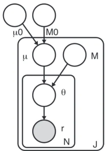
RVD2 uses a two-stage approach for detecting rare variants. First, it estimates the parameters of a hierarchical Bayesian model under two sequencing data sets: one from the sample of interest (case) and one from a known reference sample (control). Then, it tests for a significant difference between key model parameters in the case and control samples and returns called variant positions.

r θ M N _J M0 μ μ0

For a given sample, the observed data consists of two matrices r ∈ IRJ×N and

n ∈IRJ×N_{, wherer}

jiis the number of reads with a non-reference base at locationj in

experimental replicateiandnjiis the total number of reads at locationj in replicate

i. J is the region of interest length and N is the number of technical replicates in the sample. Technical replicates are used to establish experimental variability in next-generation sequencing procedure [53, 58], though multiple replicates are not necessary for RVD2.

The model generative process given hyperparametersµ0, M0 andMis as follows:

noitemsep For each location j:

(a) Draw an error rate µj ∼Beta(µ0, M0)

(b) For each replicate i:

i. Draw θji ∼Beta(µj, Mj)

ii. Draw rji|nji ∼Binomial(θji, nji)

The generative process involves several hyperparameters: µ0, a global error rate;

M0, a global precision; µj, a local error rate. Mj, a local precision. The global error

rate, µ0, estimates the expected error rate across all locations. The global precision,

M0, estimates the variation in the error rate across locations. The local error rate,

µj, estimates the exepected error rate across replicates at location j. The local

precision, Mj, estimates the variation in the error rate across replicates at location

j.

RVD2 has three levels of sampling. First, a global error rate and global precision are chosen once for the entire data set. Then, at each location, a local precision is chosen and a local error rate is sampled from a Beta distribution. Finally, the error rate for replicate i at locationj is drawn from a Beta distribution and the number

RVD2 hierarchically partitions sources of variation in the data. The distribu-tion rji|nji ∼ Binomial(θji, nji) models the variation due to sampling the pool of

DNA molecules on the sequencer. The distribution θji ∼ Beta(µj, Mj) models the

variation due to experimental reproducibility. The variation in error rate due to se-quence context is modeled by µj ∼Beta(µ0, M0). Importantly, increasing the read

depth nji only reduces the sampling error, but does nothing to reduce experimental

variation or variation due to sequence context.

Figure 2.1 shows a graphical representation of the RVD2 statistical model. The joint distribution over the latent and observed variables for data at location

j in replicatei given the parameters can be factorized as

p(rji, θji, µj|nji;µ0, M0, Mj) = p(rji|θji, nji)p(θji|µj;Mj)p(µj;µ0, M0), (2.1) where p(µj;µ0, M0) = Γ(M0) Γ(µ0M0)Γ(M0(1−µ0)) · µM0µ0−1 j (1−µj)M0(1−µ0)−1, p(θji|µj;Mj) = Γ(Mj) Γ(µjMj)Γ(Mj(1−µj)) · θMjµj−1 ji (1−θji)Mj(1−µj)−1, p(rji|θji, nji) = Γ(nji+ 1) Γ(rji+ 1)Γ(nji−rji+ 1) · θrji ji (1−θji)nji−rji. (2.2)

Integrating over the latent variables θji and µj yields the marginal distribution of the data, p(rji|nji;µ0, M0, Mj) = Z µj Z θji p(rji|θji, nji) p(θji|µj;Mj)p(µj;µ0, M0)dθjidµj. (2.3)

Finally, the log-likelihood of the data set is logp(r|n;µ0, M0, M) = J X j=1 N X i=1 log Z µj Z θji p(rji|θji, nji) p(θji|µj;Mj)p(µj;µ0, M0)dθjidµj. (2.4)

RVD2 improves on RVD in three ways. First, RVD2 has a Beta(µ0, M0) prior

on local error rateµj, which captures the global across-position error rate. The

pri-or distribution allows µj to borrow information from adjacent positions and allows

RVD2 to handle low read depths. second, this method smoothly handles multiple replicates in case samples. Third, RVD2 has a more accurate Bayesian hypoth-esis testing method compared to a frequentist normal z-test in RVD. We show a performance comparison between RVD and RVD2 in Section 4.1.3.

2.2

Sampling Inference

The primary object of inference in this model is the joint posterior distribution function over the latent variables,

p(µ, θ|r, n;φ) = p(µ, θ, r|n;φ)

where the parameters are φ_,{µ0, M0, M}.

The Beta distribution over µj is conjugate to the Binomial distribution over

θji, so we can write the posterior distribution as a Beta distribution. However,

there is not a closed form for the product of a Beta distribution with another Beta distribution, so exact inference is intractable.

Instead, we have developed a Metropolis-within-Gibbs approximate inference algorithm shown in Algorithm 1. First, the hyperparameters are initialized us-ing method-of-moments (MoM). Given those hyperparameter estimates, we sample from the marginal posterior distribution for µj given its Markov blanket using a

Metropolis-Hasting rejection sampling rule. Finally, we sample from the marginal posterior distribution for θji given its Markov blanket. Samples from θji can be

drawn from the posterior distribution directly because the prior and likelihood form a conjugate pair. This sampling procedure is repeated until the chain converges to a stationary distribution then we draw samples from the posterior distribution over latent variables.

Algorithm 1 Metropolis-within-Gibbs Algorithm

1: Initialize θ,µ, M, µ0, M0

2: repeat

3: for each location jdo

4: Draw T samples from p(µj|θij, µ0, M0) using M–H

5: Set µj to the sample median for the T samples

6: for each replicate i do

7: Sample from p(θij|rij, nij, µj, M)

8: end for

9: end for

2.2.1

Initialization

The initial values for the model parameters and latent variables is obtained by a method-of-moments (MoM) procedure. MoM works by setting the population moment equal to the sample moment. A system of equations is formed such that the number of moment equations is equal to the number of unknown parameters and the equations are solved simultaneously to give the parameter estimates. We simply start with the data matrices r and n and work up the hierarchy of the graphical model solving for the parameters of each conditional distribution in turn.

We present the initial parameter estimates here and provide the derivations in Supplementary Information. The MoM estimate for replicate-level parameters are

ˆ

θji = rji

nji. The estimates for the position-level parameters are ˆµj =

1 N PN i=1θˆji and ˆMj = ˆ µj(1−ˆµj) 1 N PN i=1θˆji2

−1. The estimates for the genome-level parameters are ˆµ0 = 1 J PJ j=1µˆj and ˆM0 = ˆ µ0(1−ˆµ0) 1 J PJ j=1µˆ2j −1.

2.2.2

Sampling from

p

(

θ

|

r

, n

, µ

, M

)

Samples from the posterior distribution p(θji|rji, nji, µj, Mj) are drawn analytically

because of the Bayesian conjugacy between the prior p(θji|µj, Mj) ∼ Beta(µj, Mj)

and the likelihood p(rji|nji, θji)∼Binomial(θji, nji). The posterior distribution is

2.2.3

Sampling from

p

(

µ

|

θ

, M

, µ

, M

)

The posterior distribution over µj given its Markov blanket is

p(µj|θji, Mj, µ0, M0)∝p(µj|µ0, M0)p(θji|µj, Mj). (2.7)

Since the prior,p(µj|µ0, M0), is not conjugate to the likelihood,p(θji|µj, Mj), we

cannot write an analytical form for the posterior distribution. Instead, we sample from the posterior distribution using the Metropolis-Hastings algorithm.

A candidate sample is generated from the symmetric proposal distributionQ(µ∗_j|µ(_jp))_∼

N(µ(_jp), σ2

j), where µ

(p)

j is the pth from the posterior distribution. The acceptance

probability is then a= p(µ ∗ j|µ0, M0)p(θ (p+1) ji |µ ∗ j, Mj) p(µ(_jp)|µ0, M0)p(θ (p+1) ji |µ (p) j , Mj) (2.8) We fixed the proposal distribution variance for all the Metropolis-Hastings steps within a Gibbs iteration to σj = 0.1·µˆj ·(1− µˆj) if ˆµj ∈ (10−3,1−10−3) and

σj = 10−4 otherwise, where ˆµj is the MoM estimator of µj. Though it is not

theoretically necessary, we have found that the algorithm performance improves when we take the median of five or more M-H samples as a single Gibbs step for each position (More information shown in Section 5.3).

We resample from the proposal if the sample is outside of the support of the posterior distribution. We typically discard 20% of the sample for burn-in and thin the chain by a factor of 2 to reduce autocorrelation among samples (Detailed auto-correlation analysis shown in Appendix E). Since, each position j is exchangeable given the global hyperparameters µ0 and M0 this sampling step can be distributed

2.3

Variational Inference

As shown in Equation 2.5, inference in RVD2 model is the joint posterior distribution over the latent variables,

p(µ, θ|r, n;φ) = p(µ, θ, r|n;φ)

p(r|n;φ) .

Besides Metropolis-within-Gibbs sampling inference, we have developed two varia-tional inference algorithms to approximate the posterior distributionp(µ, θ|r, n;φ) [72]. Here we summarize the algorithm briefly; Appendix J provides a detailed derivation for variational inference procedure.

2.3.1

Evidence Lower Bound (ELBO)

Using Jensen’s inequality, the log-likelihood of the data is lower-bounded: logp(r|φ) = log Z µ Z θ p(r, µ, θ)dθdµ = log Z µ Z θ p(r, µ, θ)q(µ, θ) q(µ, θ)dθdµ = Z µ Z θ q(µ, θ) logp(r, µ, θ) q(µ, θ) dθdµ+ Z µ Z θ q(µ, θ) log q(µ, θ) p(µ, θ|r)dθdµ =L(q, φ) +KL(q(µ, θ)||p(µ, θ|r)) ≥ L(q, φ) (2.9)

whereφ = (µ0, M0, M),q(µ, θ) is the variational distribution.

As can be seen from Equation 2.9, the second term of log-likelihood is KL diver-gence between the variational distributionq(µ, θ) and the true posterior distribution

zero if and only if the variational distribution q(µ, θ) is exactly the true posterior distribution p(µ, θ|r). Therefore, The item L(q, φ) is the lower bound of the log-likelihood of the data. The goal of variational inference is to minimizing the KL divergence between these two distribution, but can not be done directly. Equiva-lently, we maximize the global evidence lower bound L(q, φ) in order to minimize the KL divergence.

2.3.2

Factorization

We fully factorize the exact posterior distribution using the naive mean-field method,

q(µ, θ) = q(µ)q(θ) = J Y j=1 q(µj) N Y i=1 q(θji). (2.10)

In Equation 2.10, distribution q(µj) approximate the posterior distribution of local

error rate µj in position j across replicates, while distribution θji approximate the

posterior distribution of θji, the error rate distribution in position j replicate i [4].

2.3.3

Variational Expectation-Maximization

With the conditional independence granted by proposed factorization, we are able to write out ELBO L(q, φ) in a relative simple form,

L(q, φ) = Eq[logp(r, µ, θ|n;φ)]−Eq[logq(µ, θ)]

=Eq[logp(r|θ, n)] +Eq[logp(θ|µ;M)] +Eq[logp(µ;µ0, M0)]

−Eq[logq(µ)]−Eq[logq(θ)].

(2.11) Writing out each component shows that in order to compute ELBO, we need to obtain the following expectations with respect to variational distribution: Eq[logθji],

Eq[log (1−θji)] ,Eq[logµj] ,Eq[log(1−µj)],Eq[µj] andEq

h

log Γ(Mj)

Γ(µjMj)Γ(Mj(1−µj)) i

As shown in Appendix J.3.1, we propose to use Beta distribution q(θji) ∼

Beta (δji), which proves to be the optimal variational distribution, to approximate

posterior distribution of θji. The optimal variational distribution of µj is in a

com-plex form; instead, we propose two possible distributions as variational distribution so that the expectations are computable. The first distribution is Beta distribu-tion q(µj)∼Beta (γj), which will greatly facilitate the variational inference process.

The other choice is Laplace approximation to find an optimal normal distribution

p(µj)∼N(ˆµj,−f00(ˆµj)

−1

) [72].

Next, we use a variational EM procedure [34] to maximize ELBO and find the variational parameters that give the best approximate posterior distributions. This process produces approximate maximum-likelihood estimates of the hyperparam-eters φ = {µ0, M0, M} as well. Variational EM algorithm maximizes the ELBO

using coordinate ascent inference – iteratively optimizing each variational distribu-tion while fixing the others.

Variational EM algorithm works by alternating between ELBO maximization over variational distribution q(θ, µ)(E-step) and ELBO maximization over hyper-parameters φ = {µ0, M0, M} (M-step). The inference procedure is shown in

Al-gorithm 2 and AlAl-gorithm 3, with the major difference in variational distribution

Algorithm 2 RVD2 Variational Inference: . q(θji;δji) = Beta(δji), q(µj;γj) = Beta(γj) 1: Initialize q(θ, µ) and ˆφ 2: repeat 3: repeat 4: for j = 1 to J do 5: for i = 1 to N do

6: Optimize L(q,φˆ) over q(θji;δji) = Beta(δji)

7: end for

8: end for

9: for j = 1 to J do

10: Optimize L(q,φˆ) over q(µj;γj) = Beta(γj)

11: end for

12: untilchange in L(q,φˆ) is small

13: Set ˆφ←arg max

φ L(q, φ)

14: until change in L(q,φˆ) is small

Algorithm 3 RVD2 Variational Laplace Inference

. q(θji;δji) = Beta(δji),p(µj)∼N(ˆµj,−f00(ˆµj) −1 ) 1: Initialize q(θ, µ) and ˆφ 2: repeat 3: repeat 4: for j = 1 to J do 5: for i = 1 to N do

6: Optimize L(q,φˆ) over q(θji;δji) = Beta(δji)

7: end for

8: end for

9: for j = 1 to J do

10: Construct function f(µj) with items in ELBO depending onµj;

11: Set ˆµj ←arg max µj f(µj); 12: Approximate q(µj)≈ N(ˆµj,−f00(ˆµj,φˆ) −1 ) 13: end for

14: untilchange in L(q,φˆ) is small

15: Set ˆφ←arg max

φ L(q, φ)

2.4

Hypothesis Testing

2.4.1

Posterior Distribution Test

Posterior Difference Test

Metropolis-within-Gibbs provides samples from the posterior distribution ofµj given

the case or control data. For notational simplicity, we define the random variables associated with these two distributions µcase_j and µcontrol_j and the associated samples as ˜µcase_j and ˜µcontrol_j .

A variant is called if µcase

j > µcontrolj with high confidence,

Pr(µcase_j −µcontrol_j > τ)≈ 1 NMH NMH X k=1 1µ˜case jk −˜µ control jk >τ >1−α, (2.12)

where τ is a detection threshold and 1−α is a confidence level. We draw a sample from the posterior distribution ˜µ∆_{j ,}µ˜case_j −µ˜control_j by simple random sampling with replacement from ˜µcase

j and ˜µcontrolj .

The threshold,τ, may be set to zero or optimized for a given median depth and desired MAF detection limit. The optimal τ maximizes the Matthews Correlation Coefficient (MCC),

τ∗ = arg max

τ {MCC(τ)}. (2.13)

While we are able to compute the optimal τ threshold for a test data set, in general we would not have access to τ∗. With sufficient training data, one would be able to develop a lookup table or calibration curve to set τ based on read depth and MAF level of interest. Absent this information we set τ = 0.

Posterior Somatic Test.

Posterior Somatic Test is a two-sided posterior difference test using paired control-case sample. To identify somatic mutations, we consider scenarios when the control-case(tumor) error rate is lower than the control(germline) error rate (e.g. loss-of-heterozygosity) as well as scenarios when the case(tumor) error rate is higher than the control(germline) error rate (e.g. homozygous somatic mutation). The two hypothesis tests are then Pr(µcase

j −µcontrolj > τ)>1−α and Pr(µjcase−µcontrolj < τ)>1−α. Thresholdτ is

set at zero.

Posterior Germline Test.

Posterior Germline Test is a one-sided posterior distribution test using a single control sample. We call a germline mutation if µcontrol

j ≥τ with high confidence,

Pr(µcontrol_j ≥τ)≈ 1 NMH NMH X k=1 1µ˜control jk ≥τ >1−α, (2.14)

2.4.2

χ

test for non-uniform base distribution

An abundance of non-reference bases at a position called by the posterior density test may be due to a true mutation or due to a random sequencing error; we would like to differentiate these two scenarios. We assume non-reference read counts caused by a biological mechanism results in a uniform distribution over three non-reference bases. In contrast, the distribution of counts among three non-non-reference bases caused by biological mutation would not be uniform.

We use a χ2 _{goodness-of-fit test on a multinomial distribution over the}

non-reference bases to distinguish these two possible scenarios. The null hypothesis is

H0 : p = (p1, p2, p3) where p1 = p2 = p3 = 1/3. Cressie and Read [12] identified

Pearson’s χ2_{(λ = 1) statistic, the log likelihood ratio statistic (λ= 0), the}

Freeman-Tukey statistic (λ = −1/2), and the Neyman modified statistic X2_{(λ =−2). The}

test statistic is 2nIλ = 2 λ(λ+ 1) 3 X k=1 r(_jik)   r_ji(k) E_ji(k) !λ −1  ;λ∈R, (2.15)

wherer(_jik)is the observed frequency for non-reference basekat positionj in repli-cate i and E_ji(k) is the corresponding expected frequency under the null hypothesis. Cressie and Read [12] recommended λ= 2/3 when no knowledge of the alternative distribution is available; we choose that value.

We control for multiple hypothesis testing in two ways. We use Fisher’s combined probability test [19] to combine the p-values for N replicates into a single p-value at position j, X_j2 =−2 N X i=1 ln(pji). (2.16)

Equation (2.16) gives a test statistic that follows a χ2 distribution with 2N

degrees of freedom when the null hypothesis is true. If the sample average depth is higher than 500, we use the Benjamini-Hochberg method to control the family-wise error rate (FWER) over positions that have been called by the posterior distribution test [3, 16]. The average depth threshold is set because Benjamini-Hochberg method is a highly conservative method and will remove many true calls when the read depth is not high enough.

Chapter 3

Data

We used two independent data sets to evaluate the performance of RVD2 and com-pare it with other variant calling algorithms. Synthetic DNA sequence data provides true positive and true negative positions as well as define minor allele fractions. HC-C1187 data is used to test the performance on a sequenced cancer genome with less than 100% tumor purity.

3.0.3

Synthetic DNA Sequence Data

Experimental process.

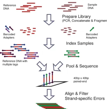
Two 400bp DNA sequences(Appendix A) that are identical except at 14 loci with variant bases were synthesized and clonally isolated and labeled case and con-trol(https://www.dna20.com). Sample of the case and control DNA were mixed at defined fractions to yield defined MAFs of 0.1%, 0.3%, 1%, 10%, and 100%. The experimental DNA synthesis and sequencing process is shown in Figure A.1. More details of the experimental protocol are available from the original publication [20].

Figure 3.1: Synthetic DNA sequence DNA sequence synthesis and sequencing flowchart. Sample and reference DNA are independently prepared and tagged with indexed adapters. The reference and sample libraries are pooled and sequenced on the same lane. The reads are aligned and preprocessed to filter out strand-specific errors [20].

Computational process.

We aligned the reads to the reference sequence using BWA v0.7.4 with the -C50 option to filter for high mapping quality reads. To simulate lower coverage data while retaining the error structure of real NGS data, BAM files for the synthetic DNA data were downsampled 10×, 100×, 1,000×, and 10,000×using Picard v1.96. The final data set contains read pairs for three replicates of each case and pairs of reads three replicates for the control sample giving N = 6 replicates for the control and each MAF level.

3.0.4

HCC1187 Sequence Data

The HCC1187 dataset is a well-recognized baseline dataset from Illumina for evalu-ating sequence analysis algorithms [29, 30, 51]. The HCC1187 cell line was derived from epithelial cells from primary breast tissue from a 41 y/o adult with TNM stage IIA primary ductal carcinoma. The estimated tumor purity was reported to be 0.8. Matched normal cells were derived from lymphoblastoid cells from peripheral blood.

Computational process.

Sequencing libraries were prepared according to the protocol described in the original technical report [2]. The raw FASTQ read files were aligned to hg19 using the Isaac aligner to generate BAM files [55]. The aligned data had an average read depth of 40x for the normal sample and 90x for the tumor sample with about 96% coverage with 10 or more reads. We used samtools mpileup to generate pileup files using hg19 as reference sequence [49].

Chapter 4

Result —

MCMC Inference

4.1

Synthetic dataset

We tested RVD2 using synthetic DNA and data from a primary ductal carcinoma sample. The Metropolis-within-Gibbs inference algorithm parameters were set to yield 4,000 Gibbs samples with a 20% burn-in and 2× tinning rate for a final total of 1,600 samples. We drew 1,000 samples from ˜µ∆_{= ˜µ}case

j −µ˜controlj to estimate the

posterior probability of a variant.

We performed posterior difference test on synthetic data to identify mutations given it is a haploid DNA sequence. We set the threshold τ = 0 and the size of the test α = 0.05. We used RVD2 to identify somatic and germline mutations in the diploid HCC1187 sample. In the posterior somatic test, we set the threshold

τ = 0 and the size of the test α = 0.05. In the posterior germline test, We set the threshold τ = 0.05 considering the low average coverage (40x). The size of the test is set at α= 0.15, higher than the size of somatic test. We are less confident on the germline test because we only use control sample in the germline test compared to normal-tumor paired sample in somatic test. We performed χ2 _{non-uniformity test}

4.1.1

Estimated MAF for variants.

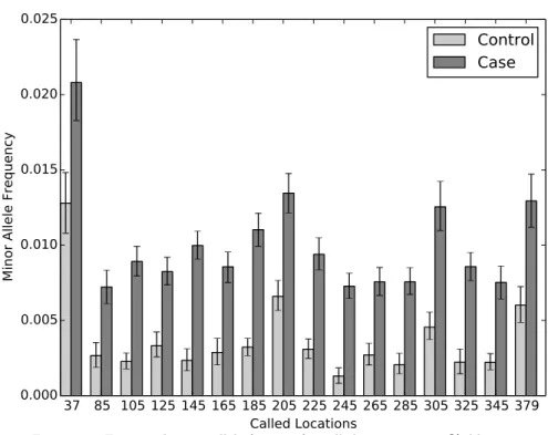
Figure 4.1 shows the posterior mean and 95% credible intervals for µj for called

variant positions with ¯n = 5584 and MAF = 1.0%. All of the called positions show a clear difference between the case and control error rates. The posterior mean estimates are all shrunken towards the global error rate parameter µ0 = 0.0023 due

to the hierarchical structure of the model.

37 85 105 125 145 165 185 205 225 245 265 285 305 325 345 379

Called Locations

0.000

0.005

0.010

0.015

0.020

0.025

Minor Allele Frequency

Control

Case

Figure 4.1: Estimated minor allele fraction for called variants in 1.0% dilution.

4.1.2

Performance with read depth

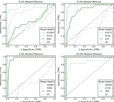
We generated receiver-operating characteristic curves (ROCs) for a range of median read depth and a range of minor allele frequencies (MAFs). For these ROC curves, we used the posterior density test without the χ2 test to evaluate the performance of posterior density test individually. Figure 4.2 shows ROC curves generated by varying the threshold τ with a fixed α = 0.05. Figure 4.2A shows ROC curves for

0.0 0.2 0.4 0.6 0.8 1.0 1-Specificity (FPR) 0.0 0.2 0.4 0.6 0.8 1.0 Sensitivity (TPR) 0.1% Mutant Mixture Read depth 41449 4129 408 39 0.0 0.2 0.4 0.6 0.8 1.0 1-Specificity (FPR) 0.0 0.2 0.4 0.6 0.8 1.0 Sensitivity (TPR) 0.3% Mutant Mixture Read depth 41472 4156 410 36 0.0 0.2 0.4 0.6 0.8 1.0 1-Specificity (FPR) 0.0 0.2 0.4 0.6 0.8 1.0 Sensitivity (TPR) 1.0% Mutant Mixture Read depth 55489 5584 535 53 0.0 0.2 0.4 0.6 0.8 1.0 1-Specificity (FPR) 0.0 0.2 0.4 0.6 0.8 1.0 Sensitivity (TPR) 10.0% Mutant Mixture Read depth 26959 2718 260 22

Figure 4.2: ROC curve varying read depth showing detection performance. Each subfigure shows ROC curves across four different read depths for one MAF level. Within one subfigurethe performance improves monotonically with read depth. Across different subfigures, the performance improves with MAF level.

a true 0.1% MAF for a range of median coverage depths. At the lowest depth the sensitivity and specificity is no better than random. However, we would not expect to be able to call a 1 in 1000 variant base with a coverage of only 43. The performance improves monotonically with read depth. Figures 4.2B-C show a similar relationship between coverage depth and accuracy for higher MAFs.

4.1.3

Performance comparison with other algorithms

We compare the empirical performance of RVD2 to other variant calling algorithms using the synthetic DNA data sets using the false discovery rate as well as sensi-tivity/specificity. Among these algorithms, Samtools and GATK are optimized for homogeneous samples, while RVD, VarScan2 Somatic, Strelka and muTect are de-signed to call variants in heterogeneous samples, which serve as better comparison

to RVD2. In a research applications, the false discovery rate is a more relevant performance metrics because the aim is generally to identify interesting variants. The sensitivity/specificity metric is more relevant in clinical applications where one is more interested in correctly calling all of the positive variants and none of the negatives. GATK, Varscan2, Strelka and muTect are only able to make use of one case and cone control sample, so we provide results of RVD2 with the same data (N = 1) for a fair comparison.

Sensitivity/Specificity Comparison

Figure 4.3 shows that samtools, GATK and VarScan2-mpileup all have similar per-formance. They call the 100% MAF experiment well even at low depth, but are unable to identify true variants in mixed samples. GATK, samtools and VarScan2-mpileup are optimized to call genotypes on pure samples. Therefore, those algo-rithms are expected to perform well on the 100% dilution (pure mutant) sample and poorly on heterogeneous samples. VarScan2-somatic is able to call more mixed samples. However, as the read depth increases the specificity degrades. Strelka is able to call 10% MAF variants with good performance, but is limited at 1% MAF and below. muTect has good performance across a wide range of MAF levels. But even at the highest depth only has around 0.5 sensitivity for low MAF levels. The statistics for RVD is an average statistics as RVD uses six control replicates to es-timate the model but returns statistics separately for three sets of pair-end case replicates. RVD performed the best among all algorithms when the read depth is as high as 40000x. RVD called all the mutated positions across all MAF levels with no false positives when MAF level is 0.3% or lower. RVD calls some false positives when the MAF level is 1.0% or higher, which causes specificity slightly lower than 1.00. RVD program fails and can not call any mutations when the depth is unable

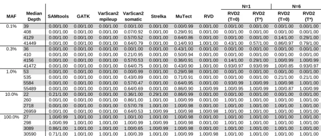
1

MAF Median

Depth SAMtools GATK

VarScan2 mpileup

VarScan2

somatic Strelka MuTect RVD

RVD2 (T=0) RVD2 (T*) RVD2 (T=0) RVD2 (T*) 0.1% 39 0.00/1.00 0.00/1.00 0.00/1.00 0.00/1.00 0.00/1.00 0.00/0.99 0.00/1.00 0.00/1.00 0.00/1.00 0.00/1.00 0.00/1.00 408 0.00/1.00 0.00/1.00 0.00/1.00 0.07/0.92 0.00/1.00 0.29/0.91 0.00/1.00 0.00/1.00 0.00/1.00 0.00/1.00 0.00/1.00 4129 0.00/1.00 0.00/1.00 0.00/1.00 0.57/0.52 0.00/1.00 0.64/0.86 0.00/1.00 0.00/1.00 0.00/1.00 0.14/1.00 0.29/1.00 41449 0.00/1.00 0.00/1.00 0.00/1.00 0.64/0.79 0.00/1.00 0.14/0.93 1.00/1.00 0.43/1.00 0.57/1.00 0.86/0.97 0.79/1.00 0.3% 36 0.00/1.00 0.00/1.00 0.00/1.00 0.00/1.00 0.00/1.00 0.43/1.00 0.00/1.00 0.00/1.00 0.00/1.00 0.00/1.00 0.00/1.00 410 0.00/1.00 0.00/1.00 0.00/1.00 0.21/0.95 0.00/1.00 0.50/0.94 0.00/1.00 0.00/1.00 0.00/1.00 0.00/1.00 0.00/1.00 4156 0.00/1.00 0.00/1.00 0.00/1.00 0.57/0.53 0.00/1.00 0.36/0.91 0.00/1.00 0.14/1.00 0.29/1.00 1.00/0.99 1.00/0.99 41472 0.00/1.00 0.00/1.00 0.00/1.00 0.64/0.75 0.00/1.00 0.43/0.90 1.00/1.00 0.93/0.97 0.93/0.99 1.00/0.85 0.93/0.97 1.0% 53 0.00/1.00 0.00/1.00 0.00/1.00 0.00/0.99 0.00/1.00 0.29/0.98 0.00/1.00 0.00/1.00 0.00/1.00 0.00/1.00 0.00/1.00 535 0.00/1.00 0.00/1.00 0.00/1.00 0.43/0.89 0.00/1.00 0.71/0.91 0.00/1.00 0.00/1.00 0.00/1.00 0.21/1.00 0.21/1.00 5584 0.00/1.00 0.00/1.00 0.00/1.00 0.57/0.47 0.00/1.00 0.64/0.95 0.00/1.00 0.93/0.99 1.00/0.99 1.00/0.98 1.00/1.00 55489 0.00/1.00 0.00/1.00 0.00/1.00 0.64/0.69 0.00/1.00 0.86/0.90 1.00/0.99 1.00/0.95 1.00/0.99 1.00/0.87 1.00/0.99 10.0% 22 0.21/1.00 0.00/1.00 0.00/1.00 0.36/1.00 0.29/1.00 0.86/0.99 0.00/1.00 0.00/1.00 0.00/1.00 0.00/1.00 0.00/1.00 260 0.00/1.00 0.00/1.00 0.00/1.00 0.86/1.00 1.00/1.00 1.00/0.99 0.00/1.00 1.00/1.00 1.00/1.00 1.00/1.00 1.00/1.00 2718 0.00/1.00 0.00/1.00 0.00/1.00 0.57/0.78 1.00/1.00 1.00/0.98 0.00/1.00 1.00/1.00 1.00/1.00 1.00/1.00 1.00/1.00 26959 0.00/1.00 0.00/1.00 0.00/1.00 0.64/0.53 1.00/0.99 1.00/0.98 1.00/0.98 1.00/1.00 1.00/1.00 1.00/1.00 1.00/1.00 100.0% 27 1.00/0.99 1.00/1.00 1.00/1.00 1.00/1.00 1.00/1.00 1.00/0.98 0.00/1.00 1.00/1.00 1.00/1.00 1.00/1.00 1.00/1.00 298 1.00/0.99 1.00/1.00 1.00/1.00 1.00/0.99 1.00/0.99 1.00/0.98 0.00/1.00 1.00/1.00 1.00/1.00 1.00/1.00 1.00/1.00 3089 0.86/1.00 1.00/1.00 1.00/1.00 1.00/0.65 1.00/0.99 1.00/0.98 0.00/1.00 1.00/1.00 1.00/1.00 1.00/1.00 1.00/1.00 30590 0.71/1.00 1.00/1.00 1.00/1.00 1.00/0.39 1.00/1.00 1.00/0.99 1.00/0.98 1.00/1.00 1.00/1.00 1.00/1.00 1.00/1.00 N=1 N=6 character_2013_03_04.xls

Figure 4.3: Sensitivity/Specificity comparison of RVD2 with other variant calling algorithms using synthetic sequence data.

to measure the baseline error rate.

The sensitivity for RVD2 withτ = 0 is low for low read depths and MAF levels and N = 1 case and control sample. The sensitivity increases considerably with read depth at a slight expense to specificity. With τ∗ the performance is much better with high sensitivity and specificity across a wide range of read depths and MAFs. However, in practice one may not know the optimalτ∗ a-priori. WithN = 6 replicates, the sensitivity increases considerably for low MAF variants with a slight degradation in specificity due to false positives. When the median read depth is at least 10× the MAF, RVD2 has higher specificity than all of the other algorithms tested and has a lower sensitivity in only three cases.

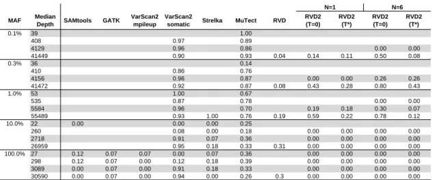
False Discovery Rate Comparison

Figure 4.4 shows the false discovery rate for RVD2 compared to samtools, GATK, varscan, Strelka and muTect. Blank cells indicate no positive calls were made.

Samtools performs well on 100% MAF sample and performance improves for read depths 3,089 and 30,590. GATK performs well on both the 10% and 100%

MAF Median

Depth SAMtools GATK

VarScan2 mpileup

VarScan2

somatic Strelka MuTect RVD

RVD2 (T=0) RVD2 (T*) RVD2 (T=0) RVD2 (T*) 0.1% 39 1.00 408 0.97 0.89 4129 0.96 0.86 0.00 0.00 41449 0.90 0.93 0.04 0.14 0.11 0.50 0.08 0.3% 36 0.14 410 0.86 0.76 4156 0.96 0.87 0.00 0.00 0.26 0.26 41472 0.92 0.87 0.08 0.43 0.28 0.80 0.43 1.0% 53 1.00 0.67 535 0.87 0.78 0.00 0.00 5584 0.96 0.70 0.19 0.18 0.30 0.07 55489 0.93 1.00 0.76 0.19 0.59 0.22 0.78 0.12 10.0% 22 0.00 0.00 0.00 0.25 260 0.08 0.00 0.18 0.00 0.00 0.00 0.00 2718 0.91 0.07 0.36 0.00 0.00 0.00 0.00 26959 0.95 0.18 0.33 0.31 0.00 0.00 0.00 0.00 100.0% 27 0.12 0.07 0.07 0.00 0.07 0.36 0.00 0.00 0.00 0.00 298 0.12 0.07 0.00 0.12 0.18 0.39 0.00 0.00 0.00 0.00 3089 0.00 0.07 0.00 0.91 0.18 0.33 0.00 0.00 0.00 0.00 30590 0.00 0.07 0.00 0.94 0.00 0.26 0.3 0.00 0.00 0.00 0.00 N=1 N=6

Figure 4.4: False discovery rate comparison of RVD2 with other variant calling algorithms using synthetic sequence data. Blank cells indicate no locations were called variant.

variants, but makes a false positive call at the 100% MAF level for all read depth levels. VarScan2-pileup performs perfectly for all but the lowest depth for the 100% MAF.

VarScan2-somatic is able to make calls for all but the lowest MAF and coverage level. However, the FDR is high due to many false positives. Interestingly, at a MAF of 100% the FDR is zero for lowest read depth and over 0.9 for the highest read depth. Strelka has a better FDR than the samtools, GATK or Varscan2-somatic algorithms for almost all read depths at the 10% and 100% MAF. However, it does not call any variants at or below 1% MAF. muTect has the best FDR performance of the other algorithms we tested over a wide range of MAF and depths. But the FDR level is relatively high at around 0.7 for 0.1% – 1% MAF and 0.3 for 10% – 100% MAF. RVD has best FDR performance in the high read depth for 0.1% – 1% MAF levels. The FDR increases to around 0.3 for 10% – 100% MAF in the high read depth.

RVD2 has a lower FDR than other algorithms when the read depth is greater than 10×the MAF withN = 1 andτset to the default value of zero or to the optimal

value. The FDR is higher whenN = 6 because the variance of the control error rate distribution P(µcontrol

j |rcontrol) is smaller. The smaller variance yields improvements

in sensitivity at the expense of more false positives. Since the FDR only considers positive calls, the performance by that measure degrades.

Matthews Correlation Coefficient Comparison

Figure 4.5 compares RVD2 with samtools, GATK, varscan, strelka and muTect using Matthews Correlation Coefficient (MCC) [45].₁

MAF Median

Depth SAMtools GATK

VarScan2 mpileup

VarScan2

somatic Strelka MuTect RVD

RVD2 (T=0) RVD2 (T*) RVD2 (T=0) RVD2 (T*) 0.1% 39 -0.02 408 -0.00 0.12 4129 0.03 0.25 0.37 0.53 41449 0.19 0.05 0.98 0.60 0.70 0.64 0.84 0.3% 36 0.60 410 0.14 0.31 4156 0.04 0.17 0.37 0.53 0.85 0.85 41472 0.16 0.19 0.95 0.71 0.81 0.41 0.71 1.0% 53 -0.02 0.29 535 0.18 0.36 0.46 0.46 5584 0.01 0.41 0.86 0.90 0.83 0.96 55489 0.13 -0.01 0.43 0.9 0.62 0.88 0.43 0.93 10.0% 22 0.46 0.59 0.53 0.79 260 0.89 1.00 0.90 1.00 1.00 1.00 1.00 2718 0.16 0.96 0.79 1.00 1.00 1.00 1.00 26959 0.06 0.90 0.81 0.82 1.00 1.00 1.00 1.00 100.0% 27 0.93 0.96 0.96 1.00 0.96 0.79 1.00 1.00 1.00 1.00 298 0.93 0.96 1.00 0.93 0.90 0.77 1.00 1.00 1.00 1.00 3089 0.92 0.96 1.00 0.25 0.90 0.81 1.00 1.00 1.00 1.00 30590 0.84 0.96 1.00 0.15 1.00 0.85 0.83 1.00 1.00 1.00 1.00 N=1 N=6 character_2013_03_04.xls

Figure 4.5: Matthews correlation coefficient (MCC) comparison with other variant calling algorithms.

Samtools and VarScan2-mpileup achieved MCC value generally higher than 0.90 on 100% MAF sample across all read depthes, with 1.0 represents for a perfect pre-diction. However, both of them detected no variant when MAF is 10.0% or lower, with only one exception for samtools when MAF is 10.0% and read depth 22. GATK, Varscan2-somatic, Strelka and GATK outperformed Samtools and VarScan2-mpile on the 10.0% MAF sample, while approximately tied in other cases. Strelka achieved best MCC on 10% MAF sample comparing to Varscan2-somatic and GATK, more specifically around 1.00 when read depth is 260 or higher. There is a very obvious

ent read depth and MAF level, a phenomenon also observed by 68. It is because VarScan2-somatic tends to call more false positives as read depth gets higher. Mu-tect seems to performs the best among all the algorithms expect RVD2 when MAF is 1.0% or lower. It achieves MCC values varying from -0.02 to 0.43, though too low to be practically meaningful. However, muTect achieved relatively lower MCC values when the MAF level is 10% and 100%, as a counteractive of being oversensitive.

RVD2 achieved MCC value 1.00 when the MAF is 100.0% at all read depth and 10% when read depth is not lower than 260. This indicates that RVD2(τ = 0, N = 1) is more accurate than the other algorithms when the median read depth is at least 10× the MAF.

4.2

HCC1187 primary ductal carcinoma sample

4.2.1

Performance of RVD2.

RVD2 identified twelve variants in the 44kbp PAXIP1 gene from chr7:154738059 to chr7:154782774. There were eight germline variants and eight somatic mutations in the twelve variants. RVD2 identified twelve variants in the 44kbp PAXIP1 gene from chr7:154738059 to chr7:154782774. There were eight germline variants and eight so-matic mutations. Figure 4.6 shows the estimated minor allele frequencies for the normal and tumor samples at the called locations. Positions chr7:154743899C>T, chr7:154749704G>A, chr7:154753635T>C, chr7:154754371T>C, chr7:154758813G>A, chr7:154766700C>A, chr7:154780960C>T, and chr7:154781769G >T were called

germline mutations. Positions chr7:154749704G>G, chr7:154753635T>C, chr7:154754371T>C, chr7:154758813G>A, chr7:154760439A>C, chr7:154766732T>G, chr7:154766832A>C,

chr7:154777118A>C were identified as significantly different in tumor and normal sample MAF and called somatic mutation. Positions chr7:154754371 and chr7:154758813

43899 rs1239326 49704 rs123932453635 rs7153417454371 rs3550551458813 60439 66700 66732 66832 77118 rs439885880960 81769 HG19 Genomic Location [chr7:154,700,000+X] 0.0 0.2 0.4 0.6 0.8 1.0

Estimate Minor Allele Frequency

*

*

*

*

*

*

*

*

¦ ¦ ¦ ¦ ¦ ¦ ¦ ¦

Control Case

Figure 4.6: Estimated minor allele fraction for Germline and Somatic mutations called by RVD2 in the 44kbp PAXIP1 gene from chr7:154738059 to chr7:154782774. Blue diamonds () indicates germline mutations, where

µcontrolis significantly different from the reference sequence. Red stars (*) indicates somatic mutations, whereµcase

is significantly different from µcontrol_{. The vertical lines represent 95% credible interval around posterior mean}

MAF. Five positions are common populations SNPs according to dbSNPv138, and the identities are shown below the positions.

appears to be loss-of-heterozygosity events. Some of these mutations are also found to be common population SNPs according to dbSNPv138. The corresponding iden-tities are shown in the Figure 4.6. The read depth distribution for positions called by RVD2 are provided in Appendix I.

4.2.2

Performance comparison with other algorithms.

We ran muTect and VarScan2-somatic to call mutations in the PAXIP1 gene in HCC1187 sample. We also compared to the result shown in original research report where Strelka was used to identify mutations in the same sample [2]. Figure 4.7a shows mutation detection result from Strelka, RVD2, muTect, and VarScan2-somatic, the state-of-art algorithms able to call mutation from heterogeneous samples. For notation simplicity, we use position index to present actual positions in Figure 4.7, while the correspondence is provided in Appendix I.

5 10 15 20 25 30 35 40 45 50 55 60 65 Position Index VarScan2 Somatic muTect RVD2 Somatic RVD2 Germline Strelka Idx:4 8 1113 2022 3537 50 5658 0 10 20 30 40 50 60 Total 60 11 8 8 1 (a)

Index REF Normal Case

A:C:G:T A:C:G:T 4 C 0:0:0:45 0:0:0:71 8 G 8:0:36:0 2:0:42:0 11 T 0:38:0:0 0:63:0:1 13 T 0:19:0:31 0:61:0:0 20 G 14:0:28:0 54:0:0:0 22 A 37:0:0:0 0:38:0:0 35 C 4:21:0:0 10:42:0:0 36 T 0:0:0:35 0:0:5:44 37 A 34:0:0:0 42:4:0:0 50 C 0:49:0:0 0:64:2:0 51 A 46:0:0:0 31:4:0:0 56 C 0:0:0:42 0:0:0:56 58 G 0:0:21:4 0:0:31:2 (b)

Figure 4.7: (a)Positions called by VarScan2-somatic, muTect, RVD2 and Strelka in the 44kbp PAXIP1 gene from chr7:154738059 to chr7:154782774. VarScan2-somatic reported 60 positions, muTect 11 positions, RVD2 12 positions and Strelka only 1 position. This figure uses position index to show the correspondence of positions called by different algorithms for notation simplicity. Complete actual positions and depth distribution are provided in Supplementary Table 1 for validation. (b) Depth distribution for positions called by RVD2 and muTect.

The mutations called by RVD2 and muTect are the most consistent among all the techniques. RVD2 detected twelve germline and somatic mutations, while muTect reported eleven, ten in common. In the disagreements, RVD2 did not call position 50 while muTect did not call position 37 and 58. Referring to the depth distribution shown in Figure 4.7b, it can be seen that position 37 and 58 are more likely mutated while position 50 is less likely mutated.

Strelka was the least sensitive algorithms among all the algorithms. According to the technical report, Strelka identified position 22 (chr7:154760439) as variant, but did not call any other variants. In particular Strelka missed the two LOH events called by RVD2. On the contrary, VarScan2-somatic called most positions among all algorithms, sixty positions as shown in Figure 4.7a. VarScan2-somatic detected all the positions called by RVD2 except position 35, which turns out to be a very likely mutation given the depth distribution in Figure 4.7b. On the other side, VarScan2-somatic reported fifty positions which were not called by any other three algorithms. The read depth in Supplementary Table 1 suggestions that these positions are very likely to be false positives. The fact that VarScan2-somatic can be over-sensitive has appeared in synthetic dataset analysis. As shown in Figure 4.4, the False Discovery

Rate for VarScan2-somatic at read depth 53 MAF level 1.0% is as high as 1.00. Spencer et al. [66] also mentioned that VarScan2 has tendency to call many false positives at high read depth.

Chapter 5

Alternative Approaches in MCMC

inference

5.1

Proposal distribution in Metropolis-Hasting

sampling

5.1.1

Detailed balance

The principle of detailed balance is that each elementary process should be equili-brated by its reverse process in the stationary state of a system. Detailed balance has been applied to many field including various MCMC methods, where equilibrium distributions are target posterior distributions [47].

In order to satisfy detailed balance in Metropolis-Hasting sampling process, a normal distribution Q(µ∗_j|µ(_jp)) _∼ N(µ(_jp), σ2_j) is used as proposal distribution to generate candidate samples for Metropolis-Hasting sampling, where µ(_jp) is the pth sample from the posterior distribution. We fixed the proposal distribution variance for all the Metropolis-Hastings steps within a Gibbs iteration toσj = 0.1·µˆj·(1−µˆj)

µj. 0 0.5 1 0 0.005 0.01 0.015 0.02 0.025 μ σ 0 2 4 6 x 10−3 0 1 2 3 4 5 6x 10 −4 μ σ

Figure 5.1: Standard deviation with respect to mean in proposal distribution Q(µ∗_j|µ(_jp)) ∼ N(µ(_jp), σ2_j) for Metropolis-Hasting sampling. The left plot is the overall plot with µ(_jp) across (0,1), while the right plot is a magnification ofµ(_jp)at the one of the two break points.

5.1.2

Obtain

σ

from

µ

ˆ

Prior to the proposal distribution described above, several other options were ex-plored. First, in stead of ˆµj, the MoM estimate of µj to provide σ, we tried it out

whether it is feasible to use the µ(_jp), the pth sample from the posterior distribu-tion. This means the proposal distribution is not fixed in standard deviation and the sampling process will violate detailed balance requirement. This is distribution was still under consideration because of two reasons: we believe it makes better proposal distribution to adjust how wide the proposal distribution is according to the mean; and Manousiouthakis and Deem [42] stated that strict detailed balance is unnecessary in Monte Carlo simulation. However, as it turned out the performance of RVD2 is slightly better when the detailed balance is met, we vetoed the proposal distribution adjusting standard deviation according to the mean.

distri-bution from the MoM estimate ˆµj. We found out that the symmetric relationship

σj = 0.1·µˆj·(1−µˆj) if ˆµj ∈(10−3,1−10−3) andσj = 10−4gives desirable acceptance

rate between 0.2-0.8.

5.2

Gibbs Sampling size

(a) (b)

Figure 5.2: Histogram ofµcontrol

j and µcasej to evaluate the sufficiency of Gibbs sampling size. The

Metropolis-Hasting sampling size is 50 in this experiment.(a)Gibbs sampling size at 400; (b)Gibbs sampling size at 4000.

The sampling inference uses Metropolis-within-Gibbs sampling approach to esti-mate the RVD2 hierarchical empirical Bayes model. However, it might require many Gibbs samples to achieve convergence and guarantee global optimal parameter set-tings. Presently there is no very good and simple ways to evaluate the convergence Gibbs sampling size. Therefore, we provide histograms of Gibbs samples of µcontrol_j

and µcase_j to intuitively evaluate the convergence of Gibbs sampling, as shown in Figure 5.2.

Figure 5.2a shows the histograms of µcontrol

j and µcasej at Gibbs sample size 400,

and Figure 5.2b shows the histograms at sample size at 4000 for position 73 and position 245, respectively. Compare the histograms in Figure 5.2a and Figure 5.2b, it can be seen that histogram at Gibbs sampling size is much smoother, which