Interface Modeling in Incompressible Media
using Level Sets in
Escript
L. Gross
a,∗
L. Bourgouin
aA. J. Hale
aH.–B. M¨
uhlhaus
a,∗
a Earth Systems Science Computational Centre (ESSCC), The University ofQueensland, St Lucia, QLD 4072, Australia.
Abstract
We use a finite element (FEM) formulation of the level set method to model geo-logical fluid flow problems involving interface propagation. Interface problems are ubiquitous in geophysics. Here we focus on a Rayleigh-Taylor instability, namely mantel plumes evolution, and the growth of lava domes. Both problems require the accurate description of the propagation of an interface between heavy and light materials (plume) or between high viscous lava and low viscous air (lava dome), re-spectively. The implementation of the models is based onEscript which is aPython module for the solution of partial differential equations (PDEs) using spatial dis-cretization techniques such as FEM. It is designed to describe numerical models in the language of PDEs while using computational components implemented in C and C++ to achieve high performance for time–intensive, numerical calculations. A critical step in the solution geological flow problems is the solution of the velocity-pressure problem. We describe how theEscript module can be used for a high–level implementation of an efficient variant of the well–known Uzawa scheme (Arrow et al., 1958). We begin with a brief outline of the Escript modules and then present illustrations of its usage for the numerical solutions of the problems mentioned above.
Key words: Partial differential equations, numerical software, level set method, Uzawa scheme, Rayleigh-Taylor instability, mantle plumes, lava dome modeling
∗ Corresponding author.
Email addresses: [email protected](L. Gross), [email protected]
(L. Bourgouin),[email protected](A. J. Hale), [email protected]
1 Introduction
Computational simulations are now firmly established as an effective tool to model and explore virtually all areas of geological fluid mechanics. This coin-cides with an unprecedented increase in the computational capacity to solve very large and complex problems. Accordingly the expectations in the com-munity in regard to sophistication and model sizes have risen significantly. There is a desire to go beyond the Stokes equations and the heat equation and to consider complex constitutive relationships, fracture, damage, chemi-cal reactions, melting, etc., all translating into additional partial differential equations.
This led to a recent trend in the development of software tools for scientific computing towards high–level user interfaces for lower level numerical libraries, see for instance Drummond et al. (to appear). The objective is to make these libraries easier to use for computational scientists and to provide an envi-ronment which is platform independent. The programming language Python
(Lutz, 2001) is the preferred environment to implement these high–level user interfaces. The main reasons for choosing Python are the facts that it is very easy to learn, even for people with very little programming background, it is widely available across all platform and a wast number of Python modules have been developed ready to use when developing new applications. More-over, Python is designed as a language to build interfaces to existing libraries developed in C or C++. In fact, there are variety of tools available which allow to make libraries callable for Python almost automatically. Although the usage of high–level, interpretive language is bearing the risk of producing inefficient code the practice has shown that, in particular if the reduced devel-opment time is taken in consideration, the losses are acceptable, mainly as the computational intensive tasks are still implemented in C/C++ and Python is used to steer the calculations only.
High–level user interfaces to numerical libraries still require the user to trans-late a mathematical model into the language of numerics. For instance, when solving partial differential equations (PDEs) using finite elements (FEM) the user still has to deal with a FEM mesh, sparse matrices and arrays to store the right hand side of a linear system, the solution and PDE coefficients. On the other hand, the user formulates the mathematical model using the termi-nology of domain, PDE and functions of spatial variables. It is the objective of Escript (Davies et al., 2004; Gross et al., to appear) to provide an envi-ronment in Python that maps the terminology used to describe PDEs–based mathematical models onto a standardised interface into which a PDE solver library written is C or C++ can be linked. The actual spatial discretization technique and its implementation which is provided by the library is hidden from the user. In particular, this allows running an implementation of a model
with different discretization methods. The abstraction from numerical tech-niques and their implementations dramatically simplifies the development of simulation codes but blocks the user from accessing individual discretization objects such as elements in the FEM mesh. However, this restriction is consis-tent with the approach of describing models using the PDE terminology which is reasonable only if there is a mesh independence in the sense of convergence towards a mesh independent solution for decreasing mesh size.
In this paper we will discuss the application of Escript to model material interfaces between incompressible media with temperature dependent viscos-ity. This class of problems are the core for many computational models in geosciences. Here we will discuss two applications, namely the formation of plumes in the Earth’s mantel and the growth of lava domes. In the case of plume formation, the interface between the heavy material in the Earth’s man-tel and the light material in the deeper manman-tel is tracked. When modelling the growth of lava domes the surface of the dome forms a free surface which is treated as an interface between lava and air. These modelling scenarios both contain three algorithmic challenges: the incompressible flow solver, the interface tracking and the advection–diffusion solver for temperature. As we want to apply Escript we are restricted in the techniques that can be used to address these challenges, in particular we cannot use special element types and element–based up-winding. In this paper we are proposing to use the in-exact Uzawa scheme as an incompressible flow solver, the level set method to track interfaces, and the two–step Taylor–Galerkin scheme to solve advection– diffusion problems. We will show how these three methods can be implemented inEscript and are successfully used to model plumes and lava domes.
In the next section we will present the governing equations and the basic idea of the level set method. Section 3 will discuss the solution algorithms that have been chosen, in particular the level set method and the inexact Uzawa scheme used as the incompressible flow solver. In Section 4 we then give a brief overview on Escript and discuss some aspects of the implementation of the solution algorithms. Section 5 will show how the model is applied to the plume formation and lava dome growth. In the final section we give a summary and outline some furtherEscript developments.
2 The Model
2.1 Governing Equations
The applications presented in this paper are governed by the Navier-Stoke’s equations for velocity vi and pressure p. We assume a linear relationship
be-tween the deviatoric stress σ0
ij and the stretching Dij = 12(vi,j +vj,i) in the
form
σ0
ij = 2η Dij0 , (1)
where η denotes the viscosity and the deviatoric stretchingD0
ij is defined as
D0
ij=Dij−
1
3Dkkδij . (2)
In this definitionδij is the Kroneckerδ-symbol and Einstein summation tensor
notation is used. We restrict ourselves to incompressible flows and neglect the inertia terms.
For gravity acting in the x3-direction the governing equations are given as
−(η(vi,j +vj,i)),j−p,i =−g ρδi3 , (3)
with the incompressibility condition
−vi,i = 0 . (4)
The coefficients ρ and g denote the density and the gravity constant, respec-tively. In equations (3) and (4) f,i denotes the derivative of the function f
with respect toxi.
The temperature field T is calculated solving the heat equation
ρcp(T,t+viT,j)−(κT,i),i=Q , (5)
wherecp is the heat capacity and κis the thermal diffusivity. The heat source
Q is given from viscous dissipation:
Q=τ γ˙ with τ = s 1 2σ 0 ijσij0 and ˙γ = q 2D0 ijD0ij . (6)
In general, the viscosity may depend on temperature and pressure but for the following discussion we assume that the temperature dependence takes the form
ln η
ηmin
= Eact Tmelt
whereEact is the activation energy, Tmelt is the melting temperature andηmin
is the minimal viscosity.
A more complex, imperical form is used in Section 5.2. We also neglect the temperature–dependency of the density but this effect can be included easily into the framework we will present.
The solution of the temperature equation (5) as well as the velocity-pressure equations (3) and (4) requires appropriate boundary conditions which for the the sake of a simpler presentation are not discussed here.
2.2 The Level Set Method
We assume that the two sub-domains Ω0 and Ω1 of the domain are filled
with two different material with distinct values for material parameter such as viscosity η and density ρ. To describe the interface Γ between the two sub-domains we use the level set method. It is based upon an implicit repre-sentation of the interface Γ by a smooth, scalar functionφ which is called the level set function. The function usually takes the form of a signed distance to the interface, whereby the zero level surface φ(x) = 0 represents the points
x on the actual interface Γ between the two materials. Points x in Ω0 can
be characterised by φ(x) < 0 while points x in Ω1 can be characterised by φ(x) > 0, or vice versa. At a given location in the domain the value of any parameter can be set depending upon the sign of φ at that location.
In the presence of a velocity field vi the interface Γ is transformed over time.
In the Eulerian framework this is described by the advection equation:
φ,t+viφ,i= 0 . (8)
It is desirable that over time the function φ maintains its initial character as a distance function. This can be expressed by the normalisation condition
φ,iφ,i = 1 . (9)
In the next section we will discuss appropriate algorithms to deal with the time-depended problems (5) and (8), the normalization condition (9) and the saddle point problem (3)-(4).
3 Algorithms
3.1 Two–Step Taylor–Galerkin Scheme
The equations (5) and (8) are written as the advection-diffusion equation
c·u,t=G(u) =f −viu,j+ (κu,i),i, (10)
where for the temperature equation (5) we set u ← T, c ← ρcp, v ← ρcpv,
f ← Q and κ ← κ, and for the advection of the level set function (8) we set
u←φ, c←1, v ←v, f ←0 and κ←0.
For time integration we use the Taylor-Galerkin scheme (Zienkiewicz & Taylor, 2000) which is of third order accuracy in time. Ifu− andu+
are the solution u
at the current and next time step anddtdenotes the time-step size the scheme can be written in the following form: First for the given solution u− at time t− one solves
c·(u1/2−u−) = dt
2G(u
−). (11)
to calculate the solutionu1/2
at the mid point t1/2
= 1 2(t
+
+t−). Then, using u1/2
, one calculates the solution u+
at the next time step t+
by solving
c·(u+
−u−) =dt G(u1/2
). (12)
In a practical implementation it is assumed that the velocity is constant for the entire time step, this means the velocity field is not updated whenG(u1/2
) is calculated.
In the case of a divergence free velocity field vi, this scheme is equivalent to
the classical one–step formulation for the pure advective case:
c·(u+−u−) =dt fˆ− dt
2c(vifˆ),i
!
with ˆf =f−viu−,i . (13)
The one–step scheme (13) and each step of the two–steps scheme (11)-(12) requires the same type of update operation but with a slightly different ex-pression for the second order spatial differential term.
To maintain stability for the Taylor–Galerkin scheme the time step size has to fulfill the Courant condition which can be written in the form
dt≤ζdt
dx2 c dx√vivi+|κ|
. (14)
This condition must be met over the entire problem domain. The value dx
is the local length scale, for instance the local element size in a finite ele-ment mesh. The factorζdt is a safety factor which is dependent on the spatial
discretization method only and is typically determined experimentally. The one–step scheme is preferred over the two–step scheme since typically it is less expensive. However, the preferred scheme ultimately depends upon the spatial discretization method. When using the finite element method the calcu-lations at each step require the solution of a system of linear of equations with the mass matrix. The computational costs can be minimised by using lumping of the mass matrix. This however can lead to instabilities. In the presence of a diffusion term, i.e. κ 6= 0, the two step scheme is the better option since the corresponding one–step scheme requires a fourth order spatial derivative which is difficult to construct in most spatial discretization schemes. In the following we will use the two–step scheme to solve the advection–diffusion problems for temperature and the advection of the level set function, but use one–step scheme for the reinitialisation of the level set function.
3.2 Reinitialisation
It is clear that in general the normalisation condition (9) of the level set func-tion φ is not preserved during the advection process. It has however been shown, see Sussman et al. (1994), that, in order to obtain acceptable conser-vation of mass, it is critical thatφ remains a distance function in regions close to any interface. Therefore, a reinitialiseialisation procedure is applied that transformsφ back into a distance functionψ but maintains the location of the interface.
We are using the following, computationally very light approach, see Sussman et al. (1994): With the artificial timet0 we are solving the initial value problem
ψ,t0 = sign(φ)(1−
q
ψ,iψ,i) and ψ(0) =φ, (15)
until the steady state is reached. The solution at the steady state will have the same zero level set as φ and meet the normalisation condition (9).
Equa-tion (15) can be rewritten as, see Tornberg & Engquist (2000):
ψ,t0 +wiψ,i = sign(φ) withwi = sign(φ) ψ,i
q
ψ,iψ,i
. (16)
Physically, equations (16) can be interpreted as the propagation of information away from the interface at the speed of wi which is a unit vector normal to
the interface and is pointing away from it.
Equation (16) is solved using the one–step Taylor–Galerkin scheme (13) where one sets
ˆ
f = sign(φ)(1−qψ,iψ,i) , (17)
If a suitable norm of ˆf is sufficiently small the steady state is reached. In practise, it not required to update the velocitywi as it is only used to stabilise
the time integration scheme. Note that the Courant condition (14) takes the simple form
dt0 ≤ζ
dt dx. (18)
The reinitialiseialisation only needs to be performed when the level set function
φ starts losing its distance function property typically, after five time steps. When the new distance function is found, the physical parameters are updated using the sign of the level set functionφ. In practise, if the values of a param-eter show a large contrast, the jump across the interface must be smoothed. The following procedure is used, to smooth the model parameter χ:
χ= χ0 whereψ <−dx χ1 whereψ > dx χ0−χ1 2dx ψ+ χ0+χ1 2 where|ψ|< dx . (19)
This has the effect that the physical parametersχ is smoothed across the in-terface on a band of width 2·dx. In the case of a finite element discretization this corresponds to a layer on one elements around the interface. The smooth-ing procedure prevents numerical instabilities due to high material parameter gradients across a single element.
3.3 Uzawa Scheme
The Uzawa scheme (Arrow et al., 1958) is used to solve the momentum equa-tion (3) with the secondary condiequa-tion (4) of incompressibility. The scheme is iterative and is based on the idea that for a given pressure p− the
momen-tum equation (3) can be used to calculate a velocity v+
. Initiallyv+
does not meet the incompressibility condition and its divergence is used to calculate an increment ∆p for the pressure as (Cahouet & Chabard, 1988)
1
η∆p=v +
i,i . (20)
The new pressure p+
given as
p+
=p−+ ∆p, (21)
is now fed back into the momentum equation (3) to calculate a new, improved velocity approximation. The iteration is completed if the relative size of the pressure increment in the L2
–norm is smaller than a given, positive tolerance
TOL: k∆pk2 ≤ TOL kp + k2 with kpk 2 2 = Z p2 dx. (22)
This criterion can be problematic in practise because slow convergence triggers termination. However, for the purpose of the paper this criterion is sufficient. A fundamental drawback of the Uzawa scheme as presented above is the fact that the new velocityv+
is calculated accurately although one can expect that the incompressibility condition will not be fulfilled. It is therefore reasonable to calculate an update increment ∆v of the current velocity approximation
v−. The increment is given as the solution of
−(η(∆vi,j+ ∆vj,i)),j =Fi+ (η(vi,j− +vj,i−)),j+p−,i , (23)
with external force
Fi =−g·ρδi3 . (24)
Then one sets
vi+ =v−
before updating the pressure. This scheme is equivalent to the classical Uzawa scheme if the incremental momentum equation is solved exactly. However, in the inexact Uzawa scheme (Bramble et al., 1997), it is sufficient to solve the incremental momentum equation (23) inexactly in the sense that a low convergence tolerance is applied in the iterative solver and/or a simplified but robust form of the left hand side operator is used. This scheme still produces fast convergence in pressure and velocity.
There are various options to modify improve efficiency and robustness of the inexact Uzawa, for instance by simplifying the left hand side operator in the equation for the velocity increment as mentioned above, and by introducing relaxation (Hu & Zou, 2001). For this paper we will restrict ourselves to the simple version presented here but want to point out that these modification are useful for the problem class discussed in this paper and that they can be implemented in the environment presented in the next section.
3.4 Work Flow
The algorithm to implement the temperature–dependent, incompressible flow with interface described by a level set function can be outlined as follows: 0. until time integration is completed:
0.0. reinitialise level set function φ from (15) by one–step scheme (13). 0.1. Update model parameter using level set function φ and smoothing (19). 0.2. Calculate new time step size dt from (14).
0.3. Until stopping criterion (22) is met:
0.3.0. Update velocityv by solving equation (23). 0.3.1. Update pressure p by solving equation (20).
0.4. Update temperature T from (5) by two–step scheme (11)–(12). 0.5. Update level set function φ from (8) by two–step scheme (11)–(12). 0.6. go to next time step.
Note that the time step size control needs to take in consideration the fact that two advection–diffusion problems, namely for the temperature and the level set function, is integrated over time. Consequently, the minimum of the upper time step size bounds required by each of the problems has to be used when performing the time step.
4 Implementation
In this section we discuss how Escript (Gross et al., to appear) is used to implement the models and solution algorithms presented above. Embedded into Python (Lutz, 2001) it provides an environment to implement mathe-matical models that are based on partial differential equations (PDEs). The functionality of Escript does not include PDE solver capabilities as such but provides an interface to PDE solver libraries. This approach achieves a high degree of reusabilty of mathematical model implementation because the code can be run with various spatial discretization techniques as well as different implementation approaches without modifications to the code.
In Escript the domain of a PDE is described by a Domain class object. The following Python script creates the Domain class object dom which is the unit cube discretized by a 10× 10×10 grid for the PDE solver library Finley
(Davies et al., 2004):
from finley import Brick dom=Brick(10,10,10)
From this code it becomes clear that a Domain class object does not only contain information about the geometry of the domain but also about the library that will be used to solve the PDEs. Implicitly this also sets the spatial discretization method. In the case ofFinley this is the finite element method (FEM).
The LinearPDE class object defines a general, second order, linear PDE over
a domain represented by a Domain class object. The general form of the PDE for an unknown vector-valued functionui represented by the LinearPDE class
is
−(Aijkluk,l+Bijkuk),j+Cikluk,l+Dikuk=−Xij,j +Yi . (26)
The coefficients A, B, C, D, X and Y are functions of their location in the domain. Moreover, natural boundary conditions of the form
nj (Aijkluk,l+Bijkuk) +dikuk =nj Xij+yi , (27)
can be defined where nj defines the outer normal field of the boundary of the
domain and y and dare given functions. Notice that A, B and X are already used in the PDE (26). To set values of ui to ri on certain locations of the
domain one can define constraints of the form
where qi is a given function defining through a positive value the locations
where the constraint is applied.
In case of a scalar solution u the PDE takes the form:
−(Ajlu,l+Bju),j+Clu,l+D u=−Xj,j+Y , (29)
with natural boundary conditions of the form
nj (Ajlu,l+Bju) +d u=nj Xj +y , (30)
and constraints of the form
u=r where q >0 . (31)
The usage of isLinearPDE class object is illustrated by solving the Helmholtz problem
−u,ll+u= 1 with nj u,j = 0 . (32)
The following script defines and solves the Helmholtz problem:
from escript import LinearPDE, kronecker pde=LinearPDE(dom)
pde.setValue(A=kronecker(dom),D=1.,Y=1.) u=pde.getSolution()
The function kronecker returns the Kronecker δ–symbol. Notice, that no special settings for the boundary conditions is required. The object u which holds the solution is an Escript Data object. InEscript Dataobject are used to represent spatial function defined on a Domain.
A closer inspection of the algorithms of Section 3 show that each time or iteration step requires the solution of a linear PDE. However, unlike in the simple Helmholtz problem the coefficients are no longer constants but become expressions involving functions of spatial coordinates. TheEscript core library provides the necessary functionality to evaluate the expressions defining the PDE coefficients inPython and to prepare the coefficients such that they can be handed over to the PDE solver library. This will discussed in more details in the following. It is pointed out that for the sake of a simpler presentation boundary conditions are ignored and in some example scripts not all variables are initialised.
4.1 The Saddle Point Problem
First we look into the implementation of Uzawa scheme as presented in Sec-tion 3.3. The following funcSec-tion solves the PDE (23) for the velocity increment ∆v and returns the result:
def getdV(v,p,eta,F): v_pde=LinearPDE(v.getDomain()) k=kronecker(v.getDomain()) kxk=outer(k,k) v_pde.setValue(A=eta*(swap_axes(kXk,1,3)+swap_axes(kXk,0,3), \ X=-eta*symmetric(grad(v))-p*kronecker(dom), \ Y=F) v_pde.setTolerance(1.e-2) dv=v_pde.getSolution() return dv
The arguments are the current velocity v and the current pressure p, the viscosity eta and the external force F. It is assumed that v and p are Data
objects. The getDomain method allows extracting their Domain.
Some care has to be taken with the selection of the smoothness of velocity and pressure. In fact, the representations have to meet the LBB condition (Girault & Raviart, 1986) which requires to use a lower approximation order for the pressure. InEscript this is reflected through the fact that although defined on the same Domain the initial value for v and p are created with two different smoothness attributes:
v=Vector(0.,Solution(dom))
p=Scalar(0.,ReducedSolution(dom))
The argument Solution indicates a PDE solution with full approximation order while argument ReducedSolution a PDE solution with reduced proximation order. In the context of second order FEM, the velocity is ap-proximated by continuous, piecewise quadratic splines while the pressure is approximated by continuous, piecewise linear splines on the same elements. Typically the pressure is represented by its values on element vertices while for velocity additionally the values at edge midpoints are used.
In the light of the concept of smoothness the calculation of the PDE coefficient
X needs special attention. When using finite elements the result of a gradient calculation is stored by its values on the quadrature points in the interior of each element as the gradient may be discontinuous. InEscript this is reflected by the fact that theData class object returned by the gradient functiongrad
to indicate the fact that a representation of the function is used which is different from the representation used for PDE solutions. The smoothness attribute of the gradient is passed through to the result of the expression
-eta*symmetric(grad(v)) (we assume that eta is just a real scalar). Then
there is aconflict with the smoothness attributeReducedSolution of the term
-p*kronecker(dom) when finally calculating the PDE coefficient X. For the
FEM the first term is stored on quadrature point while the second on element vertices. Consequently, the addition cannot performed directly but interpola-tion has to be applied before hand. In fact,Escript is detecting this mismatch of smoothness attributes and calls the interpolation functions provided by the
Domain of the arguments.
As temperature is a solution of a PDE it has the Solution smoothness at-tribute, the temperature-depending viscosity eta defined by equation (7) will also have the smoothness attributeSolution. As discussed beforeEscript will preform an interpolation of the viscosity eta when the PDE coefficient X is calculated. Similarly, as the PDE solver library will expect the coefficient Y
with smoothness attributeFunctionEscript will invoke, if required, the inter-polation of the external forceF before the coefficient is passed on to the PDE solver. It is pointed out that the function getdV can be used with a viscosity
eta being a floating point number as well as an Escript Data class object with an arbitrary smoothness attribute. The external force F can be given as aPython list of floating point numbers, anumarray object (Greenfield et al., 2002) or anEscript Dataclass object. Behind the scenes Escript performs the necessary conversions.
Typically, the PDE solver library will use an iterative method to solve a dis-crete version of the PDE. The methodsetTolerance of the LinearPDE class sets the tolerance for the solver. This is the tolerance for a given discretization and does not consider the discretization error. In the given example of the inexact Uzawa scheme we need the velocity increment with low accuracy only and therefore we require the solution of the PDE to be returned with a relative accuracy of 0.01. It requires only a few iteration steps in the PDE solver to meet this criterion.
Similar to the calculation of the velocity increment we can now easily im-plement the function getdP which returns the pressure increment by solving (20):
def getdP(v, eta):
p_pde=LinearPDE(v.getDomain()) p_pde.setReducedOn()
p_pde.setTolerance(1.e-2)
p_pde.setValue(D=1./eta,Y=div(v)) dp=p_pde.getSolution()
return dp
Although we do not solve a PDE in the strict sense, we are using theLinearPDE
class to project the discontinuous divergence of the velocity onto a continuous function. The call of the method setReducedOn makes sure that the PDE returns a solution with the smoothness attributeReducedSolution as required to meet the LBB condition. Similar to the velocity increment the PDE is solved with an accuracy of 0.01 only.
Finally the inexact Uzawa scheme can be implemented with following script which returns a new velocity v and new pressure p with toleranceTOL for the pressure:
def incompressibleFlow(v, p, eta, F, TOL=1.e-5): while L2(dp) > TOL*L2(p):
v+=getdV(v, p, eta, F) dp=getdP(v, eta)
p+=dp return v,p
The Escript function L2 is calculating the L2
–norm.
4.2 Reinitialisation
With the one–step Taylor-Galerkin scheme (13) and (17) it is simple to im-plement the reinitialiseialization of the level set function. The following
func-tion reinitialise implements the algorithm:
def reinitialise(phi, TOL=1.e-5): sgn_phi=sign(phi) v=normalize(grad(phi)) dt=0.5*inf(phi.getDomain().getSize()) pde=LinearPDE(phi.getDomain()) pde.setValue(D=1.) pde.setSolverMethod(pde.LUMPING) while L2(f_hat)>TOL: pde.setValue(X=dt/2*inner(v,f_hat),Y=f_hat) phi+=pde.getSolution()*dt f_hat=sgn_phi*(1-length(grad(phi))) return phi
The argument phi gives the current level set function while the function re-turns the reinitialised level set function describing the same interface then the input. The pseudo–time integration stops if L2
normalization condition (9) is less than the given toleranceTOL.
The method getSize of the Domain class returns the local length scale, that is the element diameter in case of the finite element method. The pseudo– time step size is determined from condition (18) withζdt = 0.5. Similar to the
pressure update calculation we are solving a PDE to calculate the level set function increment. As we are interested in the steady state solution lumping of the stiffness matrix is switched on by the call of thesetSolverMethod call. An instance of theLinearPDE is created outside the pseudo–time integration loop and all constant coefficients are set before the loop is entered. This way computational work, for instance the lumping of the stiffness matrix, has to be done once only and values can be reused during iteration.
Equation (19) defines a method to set a model parameter using a level set function. The following Python function implements this method where the argument phi is a a level set function andchi0 and chi1 are the parameter value in regions of negative values and positive values of the level set function:
def getParameter(phi, chi0, chi1): dx = phi.getDomain().getSize()
mask0 = whereNonNegative(-phi-dx)
mask1 = whereNonNegative( phi-dx)
mask01 = whereNegative(abs(phi)-dx) chi = chi0*mask0 + \
chi1*mask1 + \
((chi0-chi1)/(2*dx)*phi+(chi0+chi1)/2)*mask01 return chi
This implementation illustrate the technique of masking regions of the domain.
The whereNonNegative returns a Escript Data class object which has the
same Domain and smoothness attribute as its argument. The value is 1 in
re-gions where the argument has a non–negative value and the value 0 elsewhere. In the context of finite elements, the local length scale dx will be represented at quadrature points, that means it has the smoothness attribute Function. Therefore as phi will be interpolated the masks mask0, mask1 and mask01
inherit this attribute and consequently the returned parameter chi has the smoothness attributeFunction.
4.3 Advection–Diffusion Problem
Suppose we have an implementation of the function G the two–step scheme (11)-(12) is implemented in the following way:
u_half=u+dt/2.*G(u, kappa, v, c, Q) u=u+dt*G(u_half, kappa, v, Q)
return u
To implement the function G the LinearPDE is used:
def G(u, kappa, v, c, Q): pde=LinearPDE(u.getDomain()) g=grad(u)
pde.setValue(D=c,X=kappa*g,Y=Q-inner(v,g)) return pde.getSolution()
To speed–up the calculation one can use lumping in the evaluation ofG.
4.4 Simulation
Finally the components which have been discussed are put together where the temperature–dependent viscosity and the external force are calculated using (7) and (24). Again dropping the initialisation phase the scripts takes the following form where as example we assume that the level set function defines two region with different melting temperatures Tmelt:
while t<t_end:
phi=reinitialise(phi)
T_melt=getParameter(phi,T_melt0, T_melt1) eta=eta_min*exp(E_act*T_melt/T)
v,p=incompressibleFlow(v, p, eta, -g*rho*[0,0,1]) D=symmetric(grad(v))
dev_D=D-trace(D)/3*kronecker(3)
dt=0.5*inf(dx**2*/(dx*length(v)+abs(kappa)/rho/c_p))
T=stepAdvectionDiffusion(dt,T,kappa, rho*c_p*v, rho*c_p, \ 2*eta*length(dev_D)**2)
phi=stepAdvectionDiffusion(dt,phi,0,v) t+=dt
The implementation presented here is not the best possible as each of the subtasks creates a new instance of the LinearPDE class in every time or iter-ation step. As a LinearPDE class objects manages various structures such as the stiffness matrix pattern, the matrix entries and preconditioners it is more efficient to keep instances of the LinearPDE class and to reset modified PDE coefficient. Implementing subtasks as classes rather then functions is an ele-gant way to achieve this. In this case theLinearPDEclass objects can be stored as instance variables and an update step is implemented as a class method. As the object driven implementation requires more lines of program code we
have restricted the presentation to the simpler but less efficient approach of using function calls.
5 Applications
In this section we show how the model implementation presented in the previ-ous section is applied to the formation of plumes and the growth of lave domes. The results that are shown are from simulation runs using the OpenMP version of Escript and Finley on an SGI Altix 3700 system.
5.1 Plumes in the Earth Mantle
Plumes are defined as upwelling in the mantle driven by their own buoyancy and having the form of a large spherical head roughly 1000 km in diameter and with a narrower tail 100–200 km in diameter. They arise from the mode of convection that cools the Earth’s interior and drives plate tectonics. Plumes are active columnar upwelling, originating at hot boundary layers. They move laterally an order of magnitude slower than tectonic plates, thus generating an age-progressive chain of volcanism on the overriding plate. The basic thermal plume model has been extended to explore, for example, the effects of man-tle viscosity stratification (Leicht et al., 2001), compositional layering at the source (Farnetani, 1997), mixing within a plume (Farnetani et al., 2002), en-trained compositional buoyancy and melting at the top of the mantle (Leicht et al., 2001, 1998).
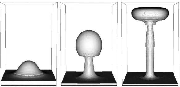
Figure 1 shows the evolution of a hot plume rising from the mantle in a box of dimension 2000 km ×2000 km ×3000 km . Initially the domain is layered by two materials: The top layer representing the Earth mantle and the bottom layer representing the hot, deeper mantle. The density and viscosity contrasts between the two layers manifest the chemical discontinuity. The temperature dependence of density and viscosity is neglected. The level set method tracks the interface between the two layers. To initiate the plume growth, an initial perturbation is prescribed in the center of the bottom layer. The model is able to reproduce realistic plume shapes. As observed in the Earth’s mantel the head of the plume is roughly 1000 km in diameter and the tail about a few hundreds kilometers.
5.2 Volcanoes
The techniques described in this paper can be applied to model lava dome growth. Here we briefly outline the usage of the presented techniques and refer to Hale et al. (in print) for more details and comparisons to the arbitrary Lagrangian–Eulerian method (ALE) used by Hale & Wadge (2003).
Figure 2 shows the geometrical set–up for an axisymmetric lava dome growth model. The lava is extruded from a conduit inlet onto the volcano surface. The conduit inlet acts as the inlet for magma flow to drive the growth of the lava dome either by prescribing a velocity or pressure boundary condition. The free–surface of the lava dome is defined as the interface between the lava and the embedding–medium air. The two subregions are modelled using the same set of equations but with different values for viscosity and density. The level set method is used to describe this interface.
The viscosity η is given in the form
η=θ·ηm , (33)
where the factor θ considers the effects of a constant crystallinity. The melt viscosityηm of the magma is calculated using an empirical equation, see Hess
& Dingwell (1996): lnη=−3.545 + 0.417·lnCf2p+ 9601−1184·ln C2 fp T −195.7 + 16.13·lnC2 fp , (34)
where Cf = 4.11 10−6P a−1 is the solubility coefficient.
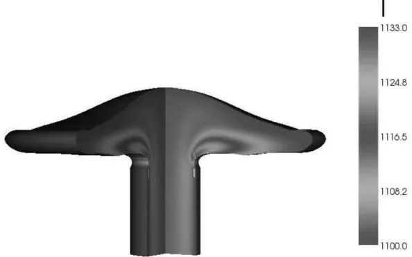
Figure 3 shows an evolving lava dome in three-dimensions. The cut–away region shows the interior temperature of the lava dome. It shows an increase in temperature from shear heating above the conduit exit. The level-set method has been proven to be a technique robust enough to model the free-surface of a growing lava dome. This technique is also computationally very light. Moreover, it does not require an initial above-ground free-surface from which the dome can be grown. As observed in Hale & Wadge (2003) assuming an initial lava free-surface shape can influence the final shape and evolution of the dome, whereas the application of the level set method avoids this complication of finding a suitable initial configuration.
6 Conclusion
TheEscript module provides an environment that allows scientists to quickly implement complex, coupled PDE–driven mathematical models. We have il-lustrated this for the example of an temperature dependent, flow of two in-compressible media. The sample script presented in Section 4.4 show how the different, independent sub–models are put together as a coupled model. In practice, the script can be easily extended by additional sub–models, for instance the advection of chemical species and chemical reactions. Coupling between sub–models is introduced through the fact the output of some models is used as the input of other models.
To simplify the coupling simple model componentsEscript provides themodelframe
environment. The basic idea is to implement each model asPython class which follows a prescribed work flow. Together with a mechanism to link parameters between models the fact that all models of a simulation apply the same work flow allows coupling models without modifying any of the model codes. If the models classes are available in libraries, a simulation can now be described by its models, the values of model parameters, the links between model parame-ters and the order in which the models are executed. This information can be captured in an XML file which then can be used to build thePython script for the simulation. The simulation description file can be created from a graphical user interface. The necessary infrastructure is currently under development.
Acknowledgment
This work is supported by Australian Computational Earth Systems Simulator Major National Research Facility, Queensland State Government Smart State Research Facility Fund, The Australian Partnership for Advanced Computing, The Queensland Cyberinfrastructure Foundation, and SGI Ltd.
References
Gross, L., Cumming, B., Steube, K. & Weatherley, D., A Python Module for PDE-based Numerical Modelling in Kagstrom, B. & Elmroth, E.,PARA’06 Proceedings, Springer–Verlag (Berlin, to appear).
Sussman, M., Smereka, P. & Osher, S., A Level Set Approach for Computing Solutions to Incompressible Two-Phase Flow, 1994, J. of Comput. Physics 114, 146–159.
Tornberg, A.-K. & Engquist, B., A finite element based level-set method for multiphase flow applications, 2000, Comput. and Visual. in Sci. 3, 93–101.
Arrow, K., Hurwicz, L., & Uzawa, H., Studies in Nonlinear Programming, Stanford University Press (Stanford, 1958).
Bramble, J.H., Pasciak, J.E. & Vassilev, A.T., Analysis of the inexact Uzawa Algorithm for saddle point problems, 1997, SIAM J. Numer. Anal. 34, 1072– 1092.
Cahouet, J. & Chabard, J.P., Some fast 3D finite element solver for the gen-eralized Stokes problem, 1988, Int. J. Numer. Meth. Fluids 8, 869–895. M. Lutz, Programming Python, 2nd edition, O’Reilly (2001).
Davies, M., Gross,L. & M¨uhlhaus, H.–B., Scripting high-performance Earth systems simulations on the SGI Altix 3700, in Proceedings of the 7th in-ternational conference on high-performance computing and grid in the Asia Pacific region, ITEE (2004).
Hu, Q. & Zou, J., An iterative method with variable relaxation parameter for saddle–point problems, 2001, SIAM J. Matrix Anal. Appl. 23. 317–338. Zienkiewicz, O.C. & Taylor, R.L., The Finite Element Method; Volume 3:
Fluid Mechanics, 5th edition, Butterworth-Heinemann (2000).
Girault, V., & Raviart, P.–A., Finite Element Methods for Navier–Stokes Equations, Springer–Verlag, (Berlin, 1986).
Greenfield, P., Miller, J.T., Hsu, J., & White., R.L., An Array Module for Python, in Bohlender, D.H., Durand, D., & Handley, T.H., Astronomical Data Analysis Software and Systems XI, Astronomical Society of the Pacific (San Francisco, 2002).
Leicht, A.M., Davies, G.F., Wells, M., A plume head melting under a rifting margin, 1998, Earth Planet. Sci. Lett. 161, 161–177.
Leicht, A.M. & Davies, G.F., Mantle plumes from flood basalts: Enhanced melting from plume ascent and an eclogite component, 2001, J. Geoph. Res. 106, 2047–2059.
Farnetani, C.G., Excess temperature of mantle plumes: the role of chemical stratification across D”, 1997, Geoph. Res. Lett. 24, 1583–1586.
Farnetani, C.G., Legras, B. & Tackley, P.J., Mixing and deformations in man-tle plumesi, 2002, Earth Planet. Sci. Lett. 196, 1–15.
Hale, A.J. & Wadge, G., Numerical modeling of the growth dynamics of a simple silicic lava dome, 2003, Geophys. Res. Letts. 30(19).
Hale H.J., Bourgouin, L., & M¨uhlhaus, H.–B., Using the Level-Set Method to Model Endogenous Lava Dome Growth, in print, J. Geophys. Res.
Hess K.U. & Dingwell, D.B., Viscosities of hydrous leucogranitic melts: A non-Arrhenian model, 1996, Am. Mineral. 81, 1297–1300.
Drummond, L., Galiano, V., Migallon, V. & Penades, J., High-level User In-terfaces for the DOE ACTS Collection, in Kagstrom, B. & Elmroth, E.,
Fig. 1. Plume raising for the deeper Earth’s mantel. Surface shows the interface between the Earth mantel and deep mantel material defined by the level set function. The resolution is 25 km.
Fig. 2. Geometrical configuration for an axisymmetric volcano with the free-surface for the initial timet= and a later timet=tnshown as a dashed line. The shaded region at the bottom-right of the domain corresponds to the surface of the volcano and has the boundary condition of zero velocity and a height of h. The radius of the conduit isa.
Fig. 3. Free-surface of a lava dome and upper conduit. The conduit radius is 15 m. Above the conduit the lava is free to flow on a flat horizontal plane. The cut-away region also shows the interior temperature of the lava dome as given by the scale.