The conservation of biodiversity is one of the most

(1)

T

he conservation of biodiversity is one of the most pressing global concerns. Numerous government and nongovernment agencies have invested large sums of money to protect species and the habitats on which they depend (Sin-clair et al. 1995). Such action is predicated on the idea that the rich diversity of life has intrinsic value that deserves protec-tion. Even so, such qualitative valuation routinely does not get appropriate weighting in policy decisions, which tend to be based on quantitative financial considerations. This problem has triggered a transformation in thinking about biodiversity conservation in terms of explicit investment opportunities that provide financial return (Daily et al. 2000). Such a change in thinking is motivated by recent scientific evidence that species collectively may provide functions in ecosystems (e.g., pro-duction, consumption, decomposition) that provide a range of services (e.g., regulation of water quality, regulation of greenhouse gases, recycling of organic wastes) vital to sus-taining life and human welfare (Costanza and Folke 1997, Costanza et al. 1997, Daily et al. 2000, Myers et al. 2000, de Groot et al. 2002, Kinzig et al. 2002). Indeed, the value of these ecosystem services may rival or exceed the value of com-modities derived from traditionally managed natural re-source sectors such as forestry, fisheries, and agriculture (Costanza and Folke 1997, Daily 1997).

A key challenge in making the idea of biodiversity con-servation through investment in ecosystem services opera-tional is empirically quantifying the link between levels of biodiversity and levels of the functions that produce a desired

ecosystem service (Daily et al. 2000). Ecological science has begun such an effort, but the focus has largely been on dis-cerning how average or expected levels of a service change with the level of biodiversity. Yet natural ecosystem function can be quite variable. This variability poses the risk that a speci-fied level of biodiversity may perform below expectations. Knowing the magnitude of such risks is as critical to invest-ment decisionmaking as is knowing the expected perfor-mance. Thus, developing an information base that enables decisionmakers to weigh competing risks requires some re-alignment in thinking about the empirical research that aims to quantify links between biodiversity and ecosystem function. The goal of this article is to show how such a realignment might be made.

To develop our case, we provide a conceptual framework that integrates linkages among biodiversity, ecosystem func-tion, and investment in the context of performance risk in much the same way as is done for portfolios of financial as-sets. This framework allows us to conceptualize biodiversity as a portfolio of natural assets (Weitzman 2000, Schläpfer et

Thomas Koellner (e-mail: [email protected]) works in the Department of Environmental Science, Natural and Social Science Interface, Swiss Federal Institute of Technology, CH-8092 Zurich, Switzerland. Oswald J. Schmitz (e-mail: [email protected]) is with the School of Forestry and Environmental Studies, Greeley Lab, Yale University, New Haven, CT 06511. © 2006 American Institute of Biological Sciences.

Biodiversity, Ecosystem

Function, and Investment Risk

THOMAS KOELLNER AND OSWALD J. SCHMITZ

Biodiversity has the potential to influence ecological services. Management of ecological services thus includes investments in biodiversity, which can be viewed as a portfolio of genes, species, and ecosystems. As with all investments, it becomes critical to understand how risk varies with the diversity of the portfolio. The goal of this article is to develop a conceptual framework, based on portfolio theory, that links levels of biodiversity and ecosystem services in the context of risk-adjusted performance. We illustrate our concept with data from temperate grassland experiments conducted to examine the link between plant species diversity and biomass production or yield. These data suggest that increased plant species diversity has considerable insurance potential by providing higher levels of risk-adjusted yield of biomass. We close by discussing how to develop conservation strategies that actively manage biodiversity portfolios in ways that address performance risk, and suggest a new empirical research program to enhance progress in this field.

Keywords: biodiversity, ecosystem services, productivity, resilience, investment risk

by guest on June 12, 2016

http://bioscience.oxfordjournals.org/

(2)

al. 2002, Baumgärtner 2005) in which biodiversity may pro-vide natural risk insurance to ecosystem managers and in-vestors. We illustrate our point using empirical information derived from past research on temperate grassland bio-diversity and its influence on the mean and variance of one important ecosystem service: plant biomass production or yield. We close by outlining the kind of research program that we believe ecologists must undertake to generate the empir-ical data necessary to support decisions on investment in the ecosystem services associated with biodiversity.

Biodiversity, variability, and performance risk We define biodiversity as the number of species contained in a system, although we recognize that the term encompasses biological types at many levels of organization beyond species in an ecosystem (e.g., genetic variety within a population of a single species). We use the species-level definition largely be-cause species tend to be the units of conservation and bebe-cause most research on ecosystem services has explored the linkage between collections of species and their associated function. We define expected performance as the mean level of an ecosystem function provided by a specific collection of species (i.e., level of biodiversity). This is quantified by averaging the magnitude of the function provided by a given collection of species across time or space. Variability in the expected per-formance can arise in two ways. First, there may be tempo-ral variability due to among-year fluctuations in the population abundance of species performing a certain func-tion within an ecosystem. Such temporal variability is often used as a surrogate measure for ecosystem stability, with the degree of variability equated with the degree of instability (Doak et al. 1998,Yachi and Loreau 1999, Lehman and Tilman 2000, Tilman et al. 2005). Second, an ecosystem function may be quite variable from location to location within a given time period, even if each location harbors the same col-lection of species. This arises simply because there is natural biological variability in the ability of individuals of all species to perform given ecosystem functions at a location.

Variability introduces the risk of poor performance for an ecosystem function. We call this underperformance risk. Such risk is quantified as the proportion of locations or time periods in which the level of an ecosystem function falls be-low the expected value. Because temporal and spatial variability lead to underperformance risk in conceptually similar ways, the arguments below apply broadly to ecological systems with variable performance.

Some effort has been made to understand the relationship between the level of biodiversity in a system and associated variability in the level of ecosystem functions. Theory predicts that higher levels of biodiversity lead to lower variability (Yachi and Loreau 1999, Lehman and Tilman 2000, Tilman et al. 2005). Systems with many species can buffer the dis-turbances better than systems with fewer species, because the probability is greater that some species will be able to main-tain a cermain-tain level of ecosystem service, even though others may fail to function. This qualitative property—the decline

in variability in ecosystem function with increasing bio-diversity—has led researchers to argue that biodiversity offers considerable insurance to managers that a particular ecosys-tem function will remain stable or persist (Yachi and Loreau 1999).

The body of theory supporting the insurance value of bio-diversity is based on conceptualizations of ecosystems as col-lections of competitor species (e.g., Lehman and Tilman 2000). That is, the theory considers only “horizontal” diver-sity (species diverdiver-sity within a particular trophic level of an ecosystem). Ecological systems contain two dimensions of species diversity, however: species diversity within trophic levels (horizontal diversity) and trophic-level diversity within ecosystems (vertical diversity). Recent research has revealed that variability in function may not always decline with in-creasing species diversity when the relationship is examined across multiple trophic levels (Halpern et al. 2005, Thébault and Loreau 2006). Thus, whether the insurance value of bio-diversity (i.e., reduction of underperformance risk) is re-tained under conditions in which variability does not decline with biodiversity depends quantitatively on the way the mag-nitude of the mean and variance in ecosystem function change with biodiversity.

Indeed, theoretically, there are many possible relationships between biodiversity and the mean and variance in ecosystem function. The mean level can increase, remain unchanged, rise and decline, or decline with increasing levels of biodiversity. The associated variance can either decrease or increase with increasing biodiversity. Accordingly, decisions about which lev-els of biodiversity offer the greatest investment opportunity require quantitative comparisons based on the mean and the variance of performance in time (i.e., volatility). If bio-diversity is considered as a portfolio of species, the analogy to portfolios of financial assets becomes evident. Several au-thors have highlighted this (Tilman et al. 1998, Lehman and Tilman 2000) and established links to the portfolio theory originally developed by Markowitz (1959). Figge (2004) has further suggested that fundamentals of portfolio theory could be used to analyze the risk–return characteristics of portfolios of species, as is done in financial asset management. Below, we outline a way to go about doing this.

Portfolio theory and investment in biodiversity The basic idea of portfolio theory is that an investor can re-duce risks purely on statistical grounds by investing in a port-folio of assets (stocks and bonds) or asset classes (countries, sectors, currencies) rather than by gambling on a single asset. A portfolio of assets has a lower collective variance when compared with the average of variances of all individ-ual assets because the variance σ2

Pof portfolio performance

is calculated as the sum of all individual variances plus all covariances (Elton and Gruber 2003):

(1)

,

(3)

where X_jis the proportion of asset jin the portfolio,σ2

jthe

variance of asset j, COV_jkthe covariance of assets jand k,and

Nthe number of assets. If the performances of individual as-sets are negatively correlated, covariances become negative and thus reduce portfolio variance. In essence, assets that are per-forming well cover for those that are perper-forming poorly. The mean performance of the portfolio µ_pis then calculated as the weighted performance X_jµ_jof each asset j:

(2)

Investment decisionmaking can be accomplished by cal-culating a risk-adjusted performance index that standardizes expected return with expected risk (Elton and Gruber 2003). One such index, the Sharpe index, quantifies risk-adjusted per-formance in terms of the ratio of expected (mean) return to variability,θ:

(3)

where µ_pis the average performance of the portfolio,R_fthe average risk-free rate of performance, and σ_pthe standard de-viation of the portfolio performance. Higher values of this in-dex are preferable to lower values because they indicate greater reliability (i.e., lower volatility or variability relative to expectations) in the performance of the investment. The Sharpe index indicates that investors should choose to take higher risks (choose portfolios with higher variances) only if they are compensated with a higher expected performance (higher mean performance). This index has considerable potential for the examination of risk in ecosystem services be-cause it uses variables that are routinely measured in ecological studies. For example, Lehman and Tilman (2000) and Tilman and colleagues (2005) used such mean-variance analysis to ex-amine the effect of plant species richness on the long-term sta-bility of plant biomass production.

Applying this type of analysis to portfolios of species re-quires ascertaining whether or not the service the species provide covaries because the species independently respond to external disturbance (e.g., differences in tolerance to drought stress among grassland species) or interact ecolog-ically (e.g., negative covariance for competitors or predators and prey and positive covariance for mutualists). It is note-worthy that ecological systems differ in one fundamental way from traditional financial systems: There is the potential for interaction among the assets (species). This potential for interactions among species means that we must consider two types of portfolios, statistical portfolios (type I) and eco-logical portfolios (type II). In type I portfolios, species, like financial assets, do not interact at all, or their interactive ef-fects can be abstracted, leading to incremental or linear changes in expected performance. A biological example might be farm-level crop diversification, in which different mono-cultures of crops are planted in different locations to protect

against risks of change in climate or in market prices. In this case, diversification is analogous to that of financial assets, and the performance of the portfolio is the average performance of each asset.

If species interact because of ecological interdepencies (a type II portfolio), then the direct analogy to financial assets breaks down. In this case, estimating the expected performance of the portfolio will require more than a simple under-standing of the relative abundance of species in the portfolio (i.e., equation 2 may not apply). It will require quantification of weightings that consider interactive effects of the partic-ular combination of species. Furthermore, species interactions may cause the relationship between species diversity in the portfolio and the mean performance of a specific function to be nonlinear.

Lehman and Tilman (2000) recognized the potential for ecological interactions to alter risk-adjusted performance and called this a covariance effect. They distinguish this from what they call the portfolio effect (i.e., variance in ecosystem function may be reduced purely on statistical grounds). How-ever, equation 1 shows that covariance is also central to ex-plaining portfolio effects. We therefore avoid using the term “covariance effect” to account for the effects of ecological interactions. Instead, we prefer to distinguish portfolios of species as either statistical (type I) or ecological (type II). Empirical examples of risk-adjusted

performance for selected ecosystems

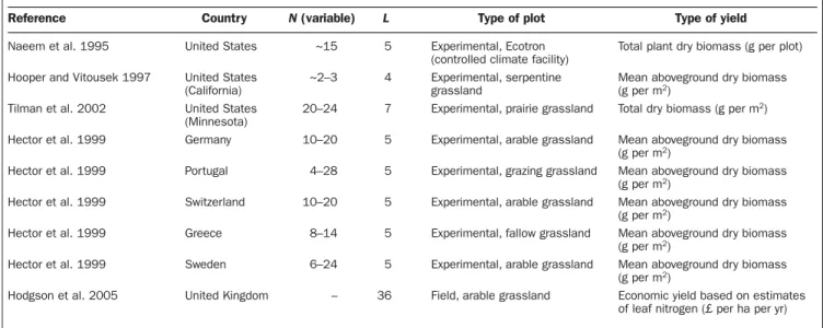
To illustrate how the risk-adjusted performance of ecosystem services varies with the level of biodiversity, we synthesized data from two kinds of studies conducted in temperate grass-lands, which are among the best-studied ecosystems (table 1). The first kind of study systematically manipulated species di-versity and measured levels of an important ecosystem ser-vice, plant biomass production or yield. The second study surveyed natural levels of biodiversity and measured the as-sociated yield within the sampling location. We analyzed the risk-adjusted performance for each kind of study separately.

Data sources.We considered the plant species within an experimental or sampling plot as a portfolio that produced a certain level of harvestable standing plant biomass or yield. To find the relationship among mean performance, variance in performance, and species diversity, we extracted data from several recent and prominent experiments reporting on the link between plant species diversity and associated produc-tivity (Hooper and Vitousek 1997, Hector et al. 1999, Tilman et al. 2002). The studies were either conducted separately within different grassland ecosystems in the United States (Hooper and Vitousek 1997, Tilman et al. 2002) or con-ducted simultaneously but replicated in different countries within continental Europe and the United Kingdom to facilitate systematic, broadscale comparison (Hector et al. 1999). In general, the experimental studies systematically manipulated the initial composition and abundance of dif-ferent plant species (biodiversity) in 4-m2_{experimental field} .

,

(4)

plots and measured the level of dry plant biomass (yield) at the end of the growing season. In all of the studies, the raw yield data for each replicate treatment were reported in graphs. We compiled our data by reading the graphs and recording all individual plot values of yield by experimental level of plant diversity. We used the compiled data to calcu-late the mean and standard deviation in yield for each ex-perimental level of plant diversity.

We also used data from Hodgson and colleagues (2005), who investigated the relationship between natural levels of plant species diversity and yield in a sample of grassland field plots in the United Kingdom. The raw data for this study were also reported graphically. In this case, plant diversity was not set at specific levels but rather varied continuously. We again recorded all individual plot values of yield from the graphs, but did this for each incremental level of plant diversity that was sampled. We then compiled the yield values ac-cording to the associated incremental level of plant species di-versity and calculated the mean and standard deviation in yield for each incremental level of diversity.

Calculation of risk-adjusted yield.We calculated the risk-adjusted yield θ_L* for a given level of biodiversity Las

(4)

where nis the number of plots with species diversity L,µ_iis the biomass yield of plot iwith diversity level L,µ_pLis the mean biomass yield of plots i= 1, ...,nat biodiversity level L,and

σpLis the standard deviation of biomass yield of plots i=

1, ...,N.In ecological systems, there is no such thing as a risk-free rate of return. We therefore obtained equation 4 by set-ting R_f(equation 3) to zero. We regressed the dependent variable, risk-adjusted yield (θ_L*), on the independent vari-able, biodiversity level (L), using SPSS 11.0 for Macintosh.

Our use of equation 4 to calculate risk-adjusted yield is merely a starting approximation to illustrate our point. More accurate quantifications of risk-adjusted yield require calcu-lating the portfolio variance according to equation 1. To do this, the biomass yield must be empirically measured in-dividually for every species (i.e., asset) of an ecological port-folio (type II) represented by plot i.Although such data are available for a few species within a common plot area, they are not, to our knowledge, available to analyze covariances for the range of plant diversities and species used in the field experiments.

Regression model for level of biodiversity and risk-adjusted yield.To analyze the risk-adjusted yield in relation to bio-diversity levels, we examined data from field plots and ex-perimental plots separately. We fit these data to several different statistical models, ranging from linear to exponen-tial, quadratic, cubic, and logarithmic. From the candidate models, we selected the four with the highest variance ex-plained (R2_{) (table 2). However, the variance explained by a}

model can be improved by increasing the number of param-eters used to fit the model. Hence, the estimated usefulness of a model must be adjusted to reflect the number of param-eters. We therefore used the Akaike information criterion (AIC) to identify the model that best explains the data, given the differences in the number of model parameters (Akaike 1973, 1985).

Table 1. Sources and types of data on number of plant species and yield for grasslands.

Reference Country N(variable) L Type of plot Type of yield

Naeem et al. 1995 United States ~15 5 Experimental, Ecotron Total plant dry biomass (g per plot)

(controlled climate facility)

Hooper and Vitousek 1997 United States ~2–3 4 Experimental, serpentine Mean aboveground dry biomass

(California) grassland (g per m2₎

Tilman et al. 2002 United States 20–24 7 Experimental, prairie grassland Total dry biomass (g per m2₎

(Minnesota)

Hector et al. 1999 Germany 10–20 5 Experimental, arable grassland Mean aboveground dry biomass

(g per m2₎

Hector et al. 1999 Portugal 4–28 5 Experimental, grazing grassland Mean aboveground dry biomass

(g per m2₎

Hector et al. 1999 Switzerland 10–20 5 Experimental, arable grassland Mean aboveground dry biomass

(g per m2₎

Hector et al. 1999 Greece 8–14 5 Experimental, fallow grassland Mean aboveground dry biomass

(g per m2₎

Hector et al. 1999 Sweden 6–24 5 Experimental, arable grassland Mean aboveground dry biomass

(g per m2₎

Hodgson et al. 2005 United Kingdom – 36 Field, arable grassland Economic yield based on estimates

of leaf nitrogen (£ per ha per yr) £, British pound sterling.

Note: Nis the number of replicates per treatment, and Lis the number of treatment levels (number of species) from which the risk-adjusted yield was calculated.

,

(5)

To assess the incremental rate of performance on invest-ment in biodiversity, we calculated the marginal rate of risk-adjusted yield as a function of diversity by taking the derivative of the functions describing risk-adjusted yield (θ*) in relation to biodiversity level (S,number of plant species):δθ*/δln S.

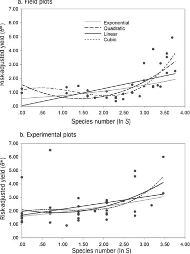
Empirical relationships between biodiversity and risk-adjusted yield for grassland ecosystems.In general, we found a tendency for risk-adjusted yield to vary concavely with bio-diversity level. The field sample data revealed a much clearer functional relationship between biodiversity and risk-adjusted yield than did data from field experiments (figure 1). Using the AIC values to compare models, it appears that the expo-nential model gives the best fit in relation to the number of parameters in the model (i.e., lowest AIC scores) (table 2). However, an analysis ofR2_{change of the nested models}

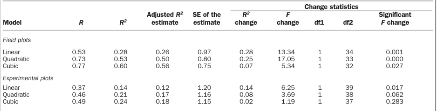
(lin-ear, quadratic, cubic) reveals that the inclusion of more vari-ables results in an increase of the R2_{with a significant change}

of the F value (table 3). Regardless, the emerging insight is that risk-adjusted yield changes nonlinearly rather than linearly with plant species diversity.

Another useful measure for decisionmaking is the incre-mental change in performance, or the marginal rate of risk-adjusted yield. In the context of our analysis, this quantifies the relative improvement in risk-adjusted yield offered by a higher level of diversity. The measure is obtained by taking the derivatives of the regression models, presented in figure 2. Here positive values indicate an incremental increase in risk-adjusted yield with diversity, zero values indicate no incre-mental change in risk-adjusted yield, and negative values indicate an incremental decrease in risk-adjusted yield. For the two best-fit models (exponential and quadratic), it appears that the marginal benefit of biodiversity does not consis-tently increase over the entire domain of available plant di-versity. Rather, it first declines (becomes more negative) before it rises (becomes more positive) (figure 2). The im-plication here is that monocultures (the lowest diversity) can offer the same marginal benefit as moderate levels of

bio-diversity. Moreover, levels of biodiversity between the lowest and moderate values will be a less preferable investment

Table 2. Regression models with risk-adjusted yield (θ*) depending on the number of plant species,S(ln S), for field plots and experimental plots.

Model R2 _df _F _p _b 0 b1 b2 b3 AIC Field plots Linear 0.28 34 13.35 0.001 0.03 0.62 – – 3.59 Exponential 0.26 34 11.78 0.002 0.55 0.33 – – 2.47 Quadratic 0.53 33 18.35 0.000 1.57 –1.42 0.50 – 3.22 Cubic 0.60 32 15.62 0.000 1.15 0.81 –1.04 0.27 3.12 Experimental plots Linear 0.14 39 6.25 0.017 1.67 0.45 – – 4.12 Exponential 0.20 39 9.22 0.004 1.59 0.19 – – 1.95 Quadratic 0.21 38 5.18 0.010 2.09 –0.55 0.33 – 4.07 Cubic 0.24 37 3.87 0.004 1.93 0.58 –0.64 0.20 4.10

AIC, Akaike information criterion; df, degrees of freedom.

Note:Linear model:θ* = b₀+ b₁ln S.Exponential model:θ* = b₀eb1 • ln S_{. Quadratic model:}_θ_{* =}_b

0+ b1ln S+ b2•

(ln S)2_{. Cubic model:}_θ_{* =}_b

0+ b1ln S+ b2• (ln S)2+ b3(ln S)3.

Figure 1. Dependency of risk-adjusted yield (θ*) and number of plant species,S(ln S), in grassland. Linear, exponential, qua-dratic, and cubic models were fitted to the data for (a) economic yield, based on leaf nitrogen measured for field plots (36 data points), and (b) biomass yield, measured for experimental plots (41 data points).

(6)

choice because they have very low prospects for risk mitiga-tion. Whether this pattern holds for many other biodiversity portfolios remains uncertain and will depend quantitatively on the way the mean and variance in performance change with biodiversity levels. The point to underscore here is that ana-lyzing the marginal rate of risk-adjusted yield can lead to conclusions about the investment opportunity in biodiversity that are altogether different from those obtained by simply analyzing the way mean performance changes with bio-diversity, as is currently done in most ecological studies.

Portfolio management for biodiversity

The results presented above show that an increased level of biodiversity can improve the yield-to-variance ratio and in-crease the marginal benefit of adding biodiversity to a port-folio. Therefore, grassland portfolios consisting of plots with higher plant species diversity can provide risk mitigation with respect to biomass production. There is one caveat, however: We did not investigate whether mixed (i.e., struc-tured) portfolios of plots with high and low diversity levels may offer even better mitigation. Nonetheless, we now have an analytical framework to gauge which kinds of biodiversity portfolios (combinations of biodiversity plots) can optimize the expected performance-to-variance ratio. Thus, invest-ment risk mitigation may be considered another environ-mental service of biodiversity. This contradicts certain contemporary viewpoints that there is a necessary trade-off between biodiversity and agricultural production (van Wenum et al. 2004).

By analogy to financial portfolio management, the task in ecosystem management is to optimize the yield–risk–cost structure. Yield, in our sense, refers not only to direct finan-cial performance but also to any type of service provided by ecosystems (e.g., biomass production in agriculture and forestry, carbon dioxide sequestration, flood mitigation). Risk refers to the unpredictability of future yield and is de-termined by the variance in space and time (Brachinger and Weber 1997). For example, this variance in forestry and agri-cultural production can be caused by uncertainty due to nat-ural causes (e.g., frost, hail, pests, and diseases), market conditions (e.g., demand or price changes), technical rea-sons (e.g., resistance of pests to pesticides), and management abilities to respond to such exogenous impacts (Mouron and Scholz 2005). Finally, the costs of managing a portfolio should be taken into account in investment decisions, as they reduce the absolute financial performance. The crucial question, however, is what should be the relative weighting of each asset (class) in the biodiversity portfolio to optimize the out-come with respect to yield, risk, and cost. Such information is currently lacking in the ecological literature.

Figure 2. Marginal rate of risk-adjusted yield (θ*) as a function of number of species,S(ln S), calculated by taking the derivative (ln S' = δθ*/ δ ln S)for field plots (solid line) and δθ/δ experi-mental plots (dashed line). (a) Linear model for field plots (ln S' = 0.62) and experimental plots (ln S' = 0.45); (b) exponen-tial model: field plots (ln S' = 0.19e0.33ln S_{), experimental plots}

(ln S' = 0.30e00.19ln S_{); (c) quadratic model: field plots (ln}_S'₌

–1.42 + 0.99ln S), experimental plots (ln S' = –0.55 + 0.65ln S); (d) cubic model: field plots (ln S' = 0.81 – 2.09ln S + 0.81ln S2_),

experimental plots (ln S' = 0.58 – 1.27ln S+ 0.59ln S2_).

Table 3. Test ofR2_{change between linear, quadratic, and cubic models.}

Change statistics

Adjusted R2 _{SE of the} _R2 _F _Significant

Model R R2 _estimate _estimate _change _change _df1 _df2 _F_change

Field plots Linear 0.53 0.28 0.26 0.97 0.28 13.34 1 34 0.001 Quadratic 0.73 0.53 0.50 0.80 0.25 17.05 1 33 0.000 Cubic 0.77 0.60 0.56 0.75 0.07 5.34 1 32 0.027 Experimental plots Linear 0.37 0.14 0.12 1.20 0.14 6.25 1 39 0.017 Quadratic 0.46 0.21 0.17 1.16 0.08 3.69 1 38 0.062 Cubic 0.49 0.24 0.18 1.15 0.02 1.19 1 37 0.283

df, degrees of freedom; SE, standard error.

Note: Independent variables in the linear model are constant and lognormal (ln) S;in the quadratic model, constant, ln S,and (ln S)2_{; and in the cubic}

model, constant, ln S,(ln S)2_{, and (ln}_S₎3_.

(7)

Trade-off between risk-adjusted yield and biodiversity for grassland?Another important question is whether increased biodiversity results in increased risk-adjusted performance in all cases. We explore this issue by examining in more detail the values of risk-adjusted performance estimated from the field data (Hodgson et al. 2005). Recall that these data sug-gest that for very low levels of biodiversity, the mean risk-adjusted performance (yield) first decreases with increasing species diversity (left of the minimum in figure 1a), in which case the marginal risk-adjusted yield is negative (figure 2).

Although not strongly visible in the data sets analyzed, this trade-off could presumably be observed for agricultural meadows on fertilized soils with a simplified structure (a few “crop species”) that is imposed exogenously with high levels of physical changes, fertilizer input, and irrigation. However, if the goal is not only biomass production but also protection of biodiversity, then a host of efficient solutions appears to the right of the minimum shown in figure 1. That is, for each portfolio on the left side (inefficient solutions with respect to biodiversity conservation), there is a portfolio on the right side with the same performance but with a higher level of biodiversity. If there is unrestricted opportunity to invest in grassland types that lead to higher diversity (on the right side of the minimum), there is no reason for an eco-system manager to choose a portfolio from the left side of the minimum.

This is predicated, however, on the assumption that the cost of managing for a particular biodiversity level and the financial performances of biodiversity are equal for investment options on either side of the minimum. For example, if the cost of managing for high levels of biodiversity greatly exceeds that for low biodiversity, then investing in high-biodiversity port-folios may not be the most efficient choice. This underscores that simply placing an economic value on the mean level of production or service provided by biodiversity (e.g., Costanza et al. 1997) may not be compelling enough to motivate in-vestment in biodiversity conservation, because such an effort does not adequately value the way investors’ choices are mo-tivated (Figge 2004).

Limitations of mean-variance analysis for ecosystem man-agement.We used a mean-variance analysis, which treats upside and downside risks symmetrically and assumes that risk can be assessed simply by the variance in performance in relation to expectations. This does not account for the risk tol-erance of the decisionmaker. Risk-averse decisionmakers give more weight to downside risks than to upside risks, especially if the decision outcome is irreversible. The possibility that in-vestment decisions for biodiversity are irreversible is what sets investment decisions for biodiversity conservation apart from investment decisions for stocks on securities markets. Secu-rities investments are normally reversible. A security that is excluded from a portfolio can easily be included again later, provided the company offering the stock remains in business (Figge 2004). On large spatial scales—for example, on national levels—the divestments in biodiversity can lead to definitive

exclusion (i.e., extinction) of a species from a country’s port-folio (Swanson 1992), thereby eliminating future options to add the species to a portfolio.

If predictions of risk are based on a distribution that is not empirically well characterized, one encounters the problem that extreme events occur more frequently than would be pre-dicted from the model. From an investor’s point of view, such rare events represent an unpredictable risk, or dread risk (Gigerenzer 2004). Because such rare events can occur in environmental systems, measures need to be developed in ad-dition to the standard deviation to quantify the dread risks. To account for differences between upside and downside risks, specific measures were developed in the investment sector, based on probability-weighted functions of devia-tions below some threshold value (Roy 1950, Fishburn 1977, Harlow and Rao 1989). Grootveld and Hallerbach (1999), however, stress the computational difficulties of calculating downside portfolio risks and conclude that differences among downside risk measures are large compared with differences between mean–variance and downside risk measures.

The calculation of efficient frontiers, minimum-risk fron-tiers, and sophisticated downside risk measures of biodiver-sity portfolios would be a fascinating field for future research. The need for large and consistent data sets with which to cal-culate accurately the mean and variance in the level of an ecosystem service currently limits such developments. This limitation brings us to a final question, namely, what can ecol-ogists do to enhance the utility of scientific data in increas-ing interest in investment opportunities for biodiversity conservation?

Data needs and contributions of ecological research The insights we present here have significant implications for ecological field research. Ecologists examining relationships between biodiversity and ecosystem function routinely con-duct experiments using analysis of variance (ANOVA). This experimental approach often has two limitations. First, in-vestigators tend to homogenize background variation among plot sites in order to maximize the likelihood of detecting a treatment (biodiversity) effect, should one occur. As such, in-vestigators may not examine the full range of environmen-tal conditions in which different combinations of species coexist, and so may end up suppressing the magnitude of vari-ation in response (level of ecosystem function) that might oc-cur under natural conditions. This claim is borne out by the fact that the field survey data led to better quantitative reso-lution of the pattern in the risk-adjusted yield in relation to plant species diversity than did the experimental data (figure 2). In essence, ANOVA-style field experiments risk under-estimating the magnitude of variation in function, which in turn leads to an underestimate of performance risk. Second, many experiments are designed to test for an effect rather than to quantify a function and its variance. For example, exper-iments often are designed only to compare single-species treatments (low diversity) against multiple-species treat-ments (high diversity), and do not consider intermediate

(8)

pairwise, three-way, and other species combinations. Such de-signs are insufficient to quantify the covariance term (equa-tion 1) needed for accurate quantitative estimates of variance. To improve the contribution of ecological science to this area of conservation, there is a critical need for detailed in-formation on mean and variance in the level of a function across a continuous range of species diversity. Moreover, measurements should be made across a range of biophysical conditions in which a particular collection of species that con-tribute to a desired function coexist. To this end, we recom-mend that ecologists adopt regression or related response surface designs (Inouye 2001) that quantify the functional re-lationship between biodiversity and corresponding ecosystem function across a broad range of species diversity. This will al-low researchers to estimate the covariance and, ultimately, portfolio variance around each mean value accurately (risk quantification); to determine whether the variance is skewed or symmetrical (relative importance of upside or downside risk); and to estimate the ecological interdependence of species (ecological or type II portfolio). Such designs have the added advantage that they manipulate both species diversity and individual species density, thereby allowing investigators to quantify how different weightings of species (based on relative species abundance) influence risk. The insights pre-sented above deal with short-term performance in small grassland plots. The concepts we present apply to longer-term time horizons (multiyear to decades), timescales on which most economic decisions are made. However, sys-tematic experimental data on biodiversity and ecosystem performance rarely extend beyond two or three years. Con-sequently, there is a critical need for ecologists to examine per-formance over longer time periods so that the characteristics of temporal volatility and economically relevant risks can be quantified.

Such an empirical program also requires the development of rigorous theoretical frameworks to guide thinking about the economic and financial implications of the relationship between biodiversity and ecological functions generally (e.g., Lehman and Tilman 2000, Tilman et al. 2005, Thébault and Loreau 2006). Such theory can hint at where important non-linearities in field systems might arise. Moreover, it can guide the selection of functions to fit empirical diversity–function relationships measured using response surface designs (Inouye 2001) in order to foster research that leads to generalizable insights.

Conclusions

Biodiversity represents a portfolio of genes, species, and ecosystems that may contribute to vital services that sup-port human livelihoods and well-being. We have provided a general framework for understanding how biodiversity offers considerable investment potential by treating biodiversity as analagous to diversity in investment portfolios. Making this idea operational requires quantification of under-performance risk. We have shown empirically for grassland ecosystems how investment in portfolios with different

levels of biodiversity alters mean performance and under-performance risk. The conceptual framework and the ex-amples show how protecting biodiversity may require a deeper empirical understanding of not only the mean level of an ecosystem service but also its variability in time and space, thus calling for a new kind of ecological research pro-gram.

Acknowledgments

We would like to thank Simon Levin (Princeton University), Dan Esty (Yale University), Len Baker (Sutter Hill Ventures), Roland Scholz (Swiss Federal Institute of Technology, Natural and Social Science Interface [ETH-NSSI]), and Patrick Mouron (ETH-NSSI) for their critical comments. Our research was supported by funds from the Swiss National Science Foundation and the Yale University Center for Bio-diversity Conservation and Science.

References cited

Akaike H. 1973. Information theory as an extension of the maximum likelihood principle. Pages 267–281 in Petrov BN, Csaki F, eds. Proceedings of the Second International Symposium on Information Theory. Budapest (Hungary): Akademiai Kiado.

———. 1985. Prediction and entropy. Pages 1–24 in Atkinson AC, Fienberg SE, eds. A Celebration of Statistics: The ISI Centenary Volume. New York: Springer.

Baumgärtner S. 2005. The insurance value of biodiversity in the provision of ecosystem services. (28 October 2006;http://papers.ssrn.com/sol3/ papers.cfm?abstract_id=892105#)

Brachinger HW, Weber M. 1997. Risk as a primitive: A survey of measures of perceived risk. Operations Research-Spektrum 19: 235–294. Costanza R, Folke C. 1997. Valuing ecosystem services with efficiency,

fairness, and sustainability as goals. Pages 49–68 in Daly GC, ed. Nature’s Services: Societal Dependence on Natural Ecosystems. Washington (DC): Island Press.

Costanza R, et al. 1997. The value of the world’s ecosystem services and natural capital. Nature 387: 253–260.

Daily GC, ed. 1997. Nature’s Services: Societal Dependence on Natural Ecosystems. Washington (DC): Island Press.

Daily GC, et al. 2000. The value of nature and the nature of value. Science 289: 395–396.

de Groot RS, Wilson MA, Boumans RMJ. 2002. A typology for the classifi-cation, description and valuation of ecosystem functions, goods and services. Ecological Economics 41: 393–408.

Doak DF, Bigger D, Harding EK, Marvier MA, O’Malley RE, Thomson D. 1998. The statistical inevitability of stability–diversity relationships in community ecology. American Naturalist 151: 264–276.

Elton EJ, Gruber MJ. 2003. Modern Portfolio Theory and Investment Analysis. New York: Wiley.

Figge F. 2004. folio: Applying portfolio theory to biodiversity. Bio-diversity and Conservation 13: 827–849.

Fishburn PC. 1977. Mean-risk analysis with risk associated with below-target returns. American Economic Review 67: 116–126.

Gigerenzer G. 2004. Dread risk, September 11, and fatal traffic accidents. Psychological Science 15: 286–287.

Grootveld H, Hallerbach W. 1999. Variance vs downside risk: Is there really that much difference? European Journal of Operational Research 114: 304–319.

Halpern BS, Borer ET, Seabloom EW, Shurin JB. 2005. Predator effects on herbivore and plant stability. Ecology Letters 8: 189–194.

Harlow WV, Rao RKS. 1989. Asset pricing in a generalised mean-lower partial moment framework: Theory and evidence. Journal of Financial and Quantitative Analysis 3: 285–311.

(9)

Hector A, et al. 1999. Plant diversity and productivity experiments in European grasslands. Science 286: 1123–1127.

Hodgson JG, et al. 2005. How much will it cost to save grassland diversity? Biological Conservation 122: 263–273.

Hooper DU, Vitousek PM. 1997. The effects of plant composition and diversity on ecosystem processes. Science 277: 1302–1305.

Inouye BD. 2001. Response surface experimental designs for investigating interspecific competition. Ecology 82: 2696–2706.

Kinzig AP, Pacala S, Tilman D. 2002. The Functional Consequences of Biodiversity: Empirical Progress and Theoretical Extensions. Princeton (NJ): Princeton University Press.

Lehman CL, Tilman D. 2000. Biodiversity, stability, and productivity in competitive communities. American Naturalist 156: 534–552. Markowitz H. 1959. Portfolio Selection: Efficient Diversification of

Invest-ments. New York: Wiley.

Mouron P, Scholz RW. 2005. Income risk management of integrated apple orchard systems: A full cost analysis of Swiss fruit farms. Pages 23–52 in Mouron PJP. Ecological-Economic Life Cycle Management of Perennial Tree Crop Systems: The Case of Swiss Fruit Farms. DSc dissertation, Swiss Federal Institute of Technology, Zurich. Dissertation no. 15899. (5 October 2006;http://e-collection.ethbib.ethz.ch)

Myers N, Mittermeier RA, Mittermeier CG, da Fonseca GAB, Kent J. 2000. Biodiversity hotspots for conservation priorities. Nature 403: 853–858. Naeem S, Thompson LJ, Lawler SP, Lawton JH, Woodfin RM. 1995. Empir-ical evidence that declining species diversity may alter the performance of terrestrial ecosystems. Philosophical Transactions of the Royal Society B 347: 249–262.

Roy AD. 1950. Safety first and the holding of assets. Econometrica 20: 431–449.

Schläpfer F, Seidl I, Tucker M. 2002. Returns from hay cultivation in fertilized low diversity and non-fertilized high diversity grassland. An “insurance” value of grassland plant diversity? Environmental and Resource Economics 21: 89–100.

Sinclair ARE, Hik DS, Schmitz OJ, Scudder GGE, Turpin DH, Larter NC. 1995. Biodiversity and the need for habitat renewal. Ecological Applications 5: 579–587.

Swanson T. 1992. Economics of biodiversity convention. Ambio 21: 250–257. Thébault E, Loreau M. 2006. The relationship between biodiversity and

ecosystem functioning in food webs. Ecological Research 21: 17–25. Tilman D, Lehman CL, Bristow CE. 1998. Diversity–stability relationships:

Statistical inevitability or ecological consequence? American Naturalist 151: 277–282.

Tilman D, Cassman KG, Matson PA, Naylor R, Polasky S. 2002. Agricultural sustainability and intensive production practices. Nature 418: 671–677. Tilman D, Polasky S, Lehman CL. 2005. Diversity, productivity and

temporal stability in the economics of humans and nature. Journal of Environmental Economics and Management 49: 405–426.

van Wenum JH, Wossink GAA, Renkema JA. 2004. Location-specific modeling for optimizing wildlife management on crop farms. Eco-logical Economics 48: 395–407.

Weitzman ML. 2000. Economic profitability versus ecological entropy. Quarterly Journal of Economics 115: 237–263.

Yachi S, Loreau M. 1999. Biodiversity and ecosystem productivity in a fluctuating environment: The insurance hypothesis. Proceedings of the National Academy of Sciences 96: 1463–1468.