PERIOD-LUMINOSITY RELATIONS OF CEPHEID AND MIRA VARIABLES AND THEIR APPLICATION TO THE EXTRAGALACTIC DISTANCE SCALE
A Dissertation by
WENLONG YUAN
Submitted to the Office of Graduate and Professional Studies of Texas A&M University
in partial fulfillment of the requirements for the degree of DOCTOR OF PHILOSOPHY
Chair of Committee, Lucas M. Macri Committee Members, Jianhua Z. Huang
Jennifer L. Marshall Nicholas B. Suntzeff Head of Department, Peter McIntyre
August 2017
Major Subject: Physics
ABSTRACT
In this dissertation, I present work towards accurate and precise distance determina-tions using both Cepheids and Miras. The work includes a Cepheid search in the galaxy M101, a study of near-infrared light curves and phase corrections for Galactic Cepheids, a Mira search in the galaxy M33, a study of near-infrared properties of Miras in the Large Magellanic Cloud, and an investigation into the suitability of the Large Synoptic Sur-vey Telescope for detecting extragalactic Miras. Using time-series observations of two fields in M101, we identified hundreds of Cepheids and derived their mean magnitudes We obtained optical Cepheid Period-Luminosity Relations and a reddening-corrected dis-tance to this galaxy. Combining the ground-based time-series observations for 34 Galactic Cepheids with literature data, we determined the contemporary phases of a sample of Galactic Cepheids. We used the phases and light curves to correct the single-epoch space-based observations to their mean values. Collaborating with statisticians, we carried out a Mira search in the Local Group galaxy M33 by coupling a novel semi-parametric Gaus-sian process model and machine learning techniques. We discovered 1847 Mira candi-dates usingI-band measurements and obtained preliminary Period-Luminosity Relations at multiple wavelengths. We studied the near-infrared properties of Large Magellanic Cloud Mira candidates using multi-epoch J HKs observations. We found that the color
excesses of Oxygen- and Carbon-rich Miras are different and compared them with the in-terstellar extinction law. We obtained the near-infrared Mira Period-Luminosity Relations for the Oxygen-rich subtype. We investigated the feasibility of discovering Miras with the Large Synoptic Survey Telescope. We found that our method will discover a considerable number of Oxygen-rich Miras in dozens of systems within 15 Mpc.
ACKNOWLEDGMENTS
I would like to thank my PhD Advisor, Lucas Macri, for his mentorship and support during these past five years. He always gives instant yet comprehensive answers to my questions, and insightful suggestions for my research. I thank my collaborators in the Department of Statistics at Texas A&M University, Shiyuan He, Jianhua Huang, and James Long and all the members in my PhD committee. I would also like to thank my parents, sister, and wife for their constant love and support.
This research has made use of the following resources:
• the Mikulski Archive for Space Telescopes (MAST) at STScI, which is operated by the Association of Universities for Research in Astronomy, Inc., under NASA contract NAS5-26555.
• data products from the Two Micron All Sky Survey, which is a joint project of the University of Massachusetts and the Infrared Processing and Analysis Cen-ter/California Institute of Technology, funded by the National Aeronautics and Space Administration and the National Science Foundation.
• data products from the Optical Gravitational Lensing Experiment, conducted by the Astronomical Institute of the University of Warsaw at Las Campanas Observatory, operated by the Carnegie Institution for Science.
• the NASA/IPAC Extragalactic Database (NED), which is operated by the Jet Propul-sion Laboratory, California Institute of Technology, under contract with NASA.
• the variable star observations from the AAVSO International Database contributed by observers worldwide.
• the VizieR catalogue access tool, CDS, Strasbourg, France.
• the Texas A&M University Brazos HPC cluster.
CONTRIBUTORS AND FUNDING SOURCES
Contributors
This work was supported by a dissertation committee consisting of Professor Lucas Macri (advisor), Jennifer Marshall and Nicholas Suntzeff of the Department of Physics and Astronomy and Professor Jianhua Huang of the Department of Statistics.
The analyses depicted in Section 2 were conducted in part by Samantha Hoffmann of the Department of Physics and Astronomy and were published in 2016 in an article listed in the Astrophysical Journal. The analyses depicted in Section 4 were conducted in part by Lucas Macri of the Department of Physics and Astronomy and Shiyuan He, James Long, Jianhua Huang of the Department of Statistics and were published in 2017 in an article listed in the Astronomical Journal.
All other work conducted for the dissertation was completed by the student indepen-dently.
Funding Sources
Graduate study was supported by the National Science Foundation through grant AST-1211603, by the National Aeronautics and Space Administration and the Space Tele-scope Science Institute through grants HST-GO-12880, 13334, 13335 & 13678, and by the Mitchell Institute for Fundamental Physics and Astronomy at Texas A&M University.
NOMENCLATURE
2MASS Two Micron All Sky Survey
ACS Advanced Camera for Surveys
AGB Asymptotic Giant Branch
AUC Area Under the Curve
C-rich Carbon-rich
CTE Charge Transfer Efficiency
CTIO Cerro Tololo Inter-American Observatory
FLWO Fred L. Whipple Observatory
GR General Relativity
H0 Hubble constant
HR diagram Hertzsprung-Russell diagram
HST Hubble Space Telescope
LMC Large Magellanic Cloud
LMCNISS LMC Near-Infrared Synoptic Survey
LSST Large Synoptic Survey Telescope
MAST Mikulski Archive for Space Telescopes
NIR Near-Infrared
OGLE Optical Gravitational Lensing Experiment
oPLCR observed Period-Luminosity-Color Relation
O-rich Oxygen-rich
PSF Point Spread Function
RF Random Forest
ROC Receiver Operating Characteristic
RSS Residual Sum of Squares
SMC Small Magellanic Cloud
SNe Ia Type Ia Supernovae (plural)
SN Ia Type Ia Supernova
SNR Signal-to-Noise Ratio
SRV Semi-Regular Variable
WFC Wide Field Camera
WFC3 Wide Field Camera 3
ΛCDM Lambda Cold Dark Matter
TABLE OF CONTENTS
Page
ABSTRACT . . . ii
ACKNOWLEDGMENTS . . . iii
CONTRIBUTORS AND FUNDING SOURCES . . . v
NOMENCLATURE . . . vi
TABLE OF CONTENTS . . . viii
LIST OF FIGURES . . . x
LIST OF TABLES . . . xvii
1. INTRODUCTION . . . 1
1.1 Cepheids . . . 2
1.2 Miras . . . 6
1.3 Observational Cosmology . . . 9
2. A SEARCH FOR CEPHEIDS IN M101 . . . 11
2.1 Observations, Data Reduction, and Photometry . . . 11
2.1.1 Observations . . . 11
2.1.2 Data Reduction . . . 13
2.1.3 Photometry . . . 15
2.2 Cepheid Search Using Template Fitting . . . 15
2.3 The Cepheid PLRs in M101 . . . 16
3. NEAR-INFRARED LIGHT CURVES AND PHASE DETERMINATION FOR 34 GALACTIC CEPHEIDS . . . 21
3.1 Observations, Data Reduction, and Calibration . . . 21
3.1.1 Observations . . . 23
3.1.2 Data Reduction and Photometry . . . 23
3.1.3 Magnitude Calibration . . . 25
3.2 Phase Determination . . . 27
3.4 Summary . . . 35
4. MIRA SEARCH IN M33 . . . 38
4.1 Observations and Data Reduction . . . 38
4.2 Simulated M33 Light Curves . . . 42
4.2.1 Miras . . . 42
4.2.2 SRVs and “Constant” Stars . . . 45
4.3 Semi-Parametric Model for Identification and Period Determination of Miras . . . 45
4.4 Results . . . 47
4.4.1 Random Forest Classification of Miras . . . 47
4.4.2 Comparison with Other Classification Methods . . . 53
4.4.3 Mira Candidates and PLRs . . . 53
4.5 Summary . . . 61
5. NIR PROPERTIES OF MIRA CANDIDATES IN THE LMC . . . 62
5.1 Data . . . 62
5.1.1 LMCNISS Measurements . . . 62
5.1.2 OGLE-III Measurements . . . 63
5.2 The LMC Mira Color Excess . . . 63
5.3 Template Mira Light Curves and PLRs in the NIR . . . 67
5.3.1 Templates Light Curves . . . 68
5.3.2 Mira PLRs in NIR . . . 70
6. PROSPECTS FOR IDENTIFICATION OF OXYGEN-RICH MIRAS IN NEARBY GALAXIES WITH LSST . . . 78
6.1 Miras in Nearby Galaxies with LSST . . . 78
6.2 Relation Between Mira Discovery Rate and Light Curve Quality . . . 81
6.3 Simulation of O-rich Mira Light Curves . . . 83
6.4 Results . . . 86
6.4.1 SNRof the Simulated LSST Measurements . . . 86
6.4.2 Discovery Rates of O-rich Miras with LSST . . . 87
7. SUMMARY . . . 90
REFERENCES . . . 91
LIST OF FIGURES
FIGURE Page
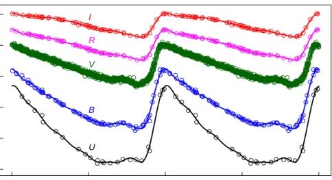
1.1 Phase-folded light curves for a classical Cepheid, VZ Pup, in U BV RI
bands. The measurements were compiled from the McMaster Cepheid Photometry and Radial Velocity Data Archive maintained by Doug Welch and the All Sky Automated Survey (Pojmanski, 1997). The solid lines represent best-fit curves with seventh-order Fourier series. . . 3 1.2 Evolutionary tracks of stars with various initial masses in the HR
dia-gram based on Schaller et al. (1992, thin solid curves) and the edges of the fundamental-mode instability strip that are estimated based on the re-sults of Alibert et al. (1999, dashed lines). The thick solid line indicates the location of the main sequence. The metallicity for the stellar models, as welll as for the edges of the instability strip, is set close to solar metallicity (Z = 0.02). Part of the material in this plot was reprinted from Schaller et al. (1992). . . 3 1.3 Distribution of periods for fundamental-mode (red) and first-overtone (blue)
Cepheids in the LMC (left) and the SMC (right). . . 4 1.4 Cepheid PLRs in the LMC in theV IJ HKsbands. TheV Imeasurements
are obtained from OGLE (Soszy´nski et al., 2008) while the J HKs
mea-surements are reprinted from Macri et al. (2015) and Persson et al. (2004). 5 1.5 The visual light curve of o Ceti from January, 2010 to April, 2017. The
data were retrieved from the American Association of Variable Star Ob-servers. . . 7 1.6 Distribution of periods for C- (red) and O-rich Miras (blue) in the LMC. . 8 2.1 The positions of all the observations superposed on Sloan Digital Sky
Sur-vey mosaic image of M101. The black boxes, blue boxes, and red boxes are corresponding to 06/07F555W-band andF814W-band observations, 2013 F555W-band and F814W-band observations, and 2013 F160W -band observations, respectively. North is up and east is to the left. . . 12
2.2 Six typical light curves for Cepheid candidates in Field 2. The top (red) and bottom (black) curves represent instrumental F814W and F555W
measurements, respectively. Circles and triangles indicate ACS and WFC3 photometry, respectively. The solid lines represent the best-fit templates using the model from Yoachim et al. (2009). . . 17 2.3 PLRs of the M101 Cepheid candidates. We excluded any objects with
periods shorter than 10 days (grey open circles). Outliers (grey points) were rejected based on the Wesenheit PLR using an iterative 2.5σclipping. The red points indicate possible Pop-II Cepheids discovered in this study. 18 2.4 Color-magnitude diagram of the Cepheid sample and field stars in M101.
Blue open circles indicate PLR outliers. Objects withE(V −I) < −0.4 mag andE(V −I)>0.75mag are indicated by blue points and red points, respectively. The symbol sizes are propotional to the periods of Cepheid candidates. The background grey dots are field stars. . . 19 2.5 Residuals of the Wesenheit PLR against [O/H] abundances for the Cepheid
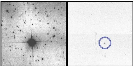
candidates in M101. We did not find any evidence of metallicity depen-dence. . . 20 3.1 Comparison ofHimage (left) andH+ND4image (right) of the same field.
In theH image, the Cepheid (brightest star) is saturated. In the H+ND4
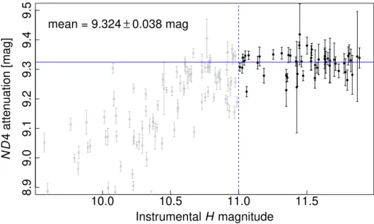
image, the Cepheid (indicated by a circle) is not saturated but no reference stars are available to derive frame-to-frame zeropoints. Slewing artifacts can be seen in the left and below the Cepheid in the right panel, and they appear in almost all of theH+ND4images. . . 24 3.2 TheND4attenuation factor versus instrumentalHmagnitude. The dashed
line indicates the approximate onset of non-linearity. The solid line shows the error-weighted mean value of theND4attenuation factor. . . 26 3.3 Hband measurements (points) and best-fit model light curves (solid lines)
for all 34 Cepheids. Two cycles of variation are plotted to aid in the visu-alization of the data. . . 27 3.4 Phase-folded light curves for AQ Pup with time-dependent period. The
time span of the measurements is more than 43 years. . . 32 3.5 Differences in periods between our determination and the GCVS values.
The black points indicate the Cepheids with constant periods while the red points indicate the Cepheids with changing periods. The gray dashed line indicates the location of zero difference. . . 33
3.6 Correlation between the absolute period-changing rates and periods for 21 Galactic Cepheids. Two Cepheids (VY Car and AQ Pup, grey points) were excluded in the fit. The solid line is the best-fit result while the dashed lines indicate the 1σscatter. . . 34 3.7 Differences in magnitude between the corrections from simulated Cepheid
light curves and the “true values” for most objects in our sample. The number below the horizontal axis is the number of ground measurements. Five variables in the sample are missing due to the lack of counterparts in the LMC with similar periods. . . 36 3.8 Ground-based light curve (black points) and best-fit model (black curve)
for XY Car. Red points indicate measurements obtained withHST. A ze-ropoint offset was applied to theHSTmeasurement to account for the dif-ference in filters. . . 37 4.1 Top: cadence of M33 observations inI by M01 and PM11. The grayscale
levels are linearly proportional to the number of measurements per square arcminute of each epoch. Bottom left: expanded view of the cadence for seasons 1–4. Bottom right: histogram of measurements for stars with N > 10 andI< 21.45 mag. . . 39 4.2 Photometric precision for secondary standards as a function of magnitude. 41 4.3 Example of a template Mira light curve and simulated M33 measurements.
Top: OGLE measurements of a Mira candidate in the LMC (black points), best-fit template using our model (blue curve), and sampling pattern of one of the M33 fields (vertical black lines). The horizontal blue arrow indicates the random shift applied to the pattern to sample the light curve. Bottom: corresponding simulated M33 light curve, including additional photometric noise. . . 44 4.4 Left: derivation of the empirical completeness function for M33
photom-etry (top: logarithmic; bottom: linear scale). An exponential model is fit to the observed luminosity function (solid black line) over the magnitude range (solid blue line) and extrapolated over the range plotted with a dot-ted blue line. The derived completeness function (solid red line) is shown in the bottom panel only. Right: magnitude distribution of Mira template light curves before (gray) and after (blue) convolution, with the complete-ness function (red line). . . 44
4.5 Examples of frequency spectra (top) and corresponding light curves (bot-tom) for a simulated Mira (left), SRV (middle), and constant star (right). The blue dashed lines and arrows indicate some of the quantities used as classification features. . . 48 4.6 Top: piecewise quadratic fit to a simulated Mira light curve. Bottom:
dis-tribution of a classification feature based on such fits for simulated Miras (blue), SRVs (red), and constant stars (black). . . 50 4.7 Distribution of RF-voted values of Mira probability (PM) for the entire
M33 sample. There are 5480 objects withPM >0.5. . . 51
4.8 Example light curves and best-fit models (solid lines) for likely Miras in M33 with different values ofPM. . . 51
4.9 RF classification of Mira candidates into O-rich (blue) or C-rich (red), plotted as a function of P and AP. Left: LMC variables classified by
Soszy´nski et al. (2009). Middle: simulated M33 variables based on the LMC sample but accounting for the shallower depth in absolute magnitude of our survey. Right: Mira candidates in M33 from this work. . . 52 4.10 Illustration of how multiple attributes help to discriminate O-rich from
C-rich Mira candidates. Left: same as right panel of Figure 4.9 but indicating the area of interest where both subtypes overlap. Middle and right: sepa-ration of candidates on other two-dimensional slices of the RF parameters. 52 4.11 ROC curves for classification between Mira/non-Mira (left) and C/O-rich
(right) for various classifiers. RF: black solid line; SLR: red dashed line; LDA: blue dotted line; SVM: green dashed-dotted line. While all classi-fiers have very similar AUCs for the first classification, RF significantly outperforms the others in the latter. . . 54 4.12 Distribution of periods (left) and amplitudes (right) for Mira candidates of
each subtype. . . 56 4.13 Deprojected distribution of Mira candidates (O-rich in black, C-rich in
red). The dashed lines indicate the boundaries of our survey. . . 56 4.14 PLRs in several bands for Mira candidates classified as O-rich in the LMC.
The solid lines show the best-fit quadratic relations to the final LMC sam-ples (large symbols) after iterative 3σ clipping of outliers (small dots). Dashed lines indicate the 1σdispersion in the fits. . . 58
4.15 PLRs in several bands for Mira candidates classified as O-rich in M33. The solid lines show the LMC-based quadratic relations of Figure 4.14 shifted by the best-fit relative distance modulus in each band (including blending correction). Small dots indicate variables removed by iterative 3σclipping. Dashed lines indicate the 1σdispersion of the Gaussian component of the model. . . 59 5.1 Example of how the mean J − H color index is derived from the three
groups of measurements for Mira candidate OGLE-LMC-LPV-08476. . . 64 5.2 Observed color-color diagram for LMC Miras. The O-rich and C-rich
sub-types are indicated by blue circles and red pluses, respectively. Outliers are indicated by grey symbols. The magenta circled cross shows the centroid of O-rich Mira color indices. The black line is the first-order best-fit for the C-rich Mira colors. . . 64 5.3 Same as Figure 5.2 but showing the intrinsic color indices of C-rich giants
from hydrostatic models (Aringer et al., 2009). Red filled circles show
M = 1M models while the green crosses indicate M = 2M models. The observed color indices of C-rich and O-rich Miras are shown in gray pluses and circles, respectively. . . 66 5.4 Correlation betweenJ −H color index and period for C-rich Miras (red
pluses). The O-rich Miras are indicated by blue circles for comparison. . 66 5.5 Observed color indices for Galactic C-rich variable stars (red dots) from
Whitelock et al. (2006), direction of reddening toward Galactic center (green solid arrow, Nishiyama et al., 2009), and direction of reddening toward Galactic K-type giants (blue dashed arrow, Wang & Jiang, 2014). The best first order best-fit of red dots is shown in black solid line. The black dashed line indicates the best-fit for the LMC C-rich Miras. . . 67 5.6 Template light curves in IJ HKs (blue curves) for Mira
OGLE-LMC-LPV-08476. The measurements are indicated by black points. . . 71 5.7 PLRs of the LMC Miras. The blue points indicate O-rich Miras while the
red points indicates C-rich Miras. The black solid lines show the best-fit quadratic relations to the O-rich Miras, while the magenta dashed lines show the PLRs based on single-epoch 2MASS observations (Yuan et al., 2017). . . 74
5.8 Correlations of PLR residuals between different bands for O-rich Miras (upper panels) and C-rich Miras (lower panels) in the LMC. We adopted the PLRs of O-rich Miras to compute the “residuals” for C-rich Miras. The black solid lines indicate the best-fit of correlations of residuals, while the black dashed lines indicate the±2σ widths of the relations. The red arrows indicate the direction of interstellar reddening based on Fouqué et al. (2007). . . 75 5.9 The oPLCRs of C-rich Miras in various combinations of bands and color
terms in the LMC. The black solid lines indicate the best-fit of correlations of residuals, while the black dashed lines indicate the ±2σ widths of the relations. Extreme outliers are indicated by gray points. . . 77 6.1 Sky coverage of the LSST main survey (blue shaded region) and the
po-sitions of the selected galaxies in the sample (red points). Within the dis-tance of 15 Mpc, 203 galaxies found from EDD that are covered by the footprint of the LSST main survey. . . 79 6.2 Simulated observation times for NGC 300 inriz and the total number of
epochs. Any measurements taken within 0.1 day are considered as a single epoch. . . 79 6.3 The color-period relation for the O-rich Miras in the LMC.V −I is based
on mean magnitudes obtained from Soszy´nski et al. (2009). The solid line indicates the best-fit and open circles are outliers. . . 81 6.4 O-rich Mira PLRs at maximum light inr (red dashed curve), i(magenta
dotted curve), and z (blue dash-dotted curve), based on tranformations fromI (black solid curve) and the period-color dependence of Miras. . . 82 6.5 O-rich Mira detection rate against SNR at maximum light (black points)
and the empirical relation between them (black curve). . . 83 6.6 Fiducial distribution of O-rich Mira periods based on the LMC and M33
samples. . . 84 6.7 Fiducial distribution of O-rich Mira amplitudes based on the LMCI-band
light curves. . . 85 6.8 Simulatedrizlight curves for a 430d-period Mira in NGC 5398, based on
the expected cadence of LSST. . . 85
6.9 Number of expected O-rich Miras to be detected by LSST (upper) and number of epochs withSN R >3(lower) as a function of Mira period in
r(black),i(red), andz (blue) bands for the galaxy NGC 4802. . . 88 6.10 Histogram of expected number of O-rich Miras that will be discovered
with LSST across all the galaxies in the sample. . . 88 6.11 Total number of Miras expected to be discovered by LSST in riz as a
LIST OF TABLES
TABLE Page
2.1 Summary of the M101 Observations . . . 14
2.2 Magnitude Calibration of M101 Photometry . . . 16
3.1 Galactic Cepheids Target List . . . 22
3.2 Phase Parameters for Cephedis with Constant Periods . . . 30
3.3 Phase Parameters for Cepheids with Time-Dependent Periods . . . 31
4.1 Features for the Classifier . . . 49
4.2 Mira Candidates in M33 . . . 55
5.1 Regression Predictors and Coefficients . . . 69
5.2 J HKsMagnitudes for LMC Miras . . . 72
5.3 O-Rich Mira PLRs in the LMC . . . 74
5.4 NIR Observed PLCRs for C-Rich Miras . . . 77
6.1 Values of Time-Independent Variables inSNRModel . . . 87
1. INTRODUCTION
Since the discovery of the expanding Universe by Hubble (1929), astronomers have endeavored to improve the measurement of its expansion rate, known as the Hubble con-stant (H0), in terms of accuracy and precision. H0 is defined as the apparent recession
velocity of an object located at unit distance in the present-day Universe. The state-of-the-art method to measure H0 is through a cosmic distance ladder, calibrating each rung
using overlapping distance indicators. Geometric methods, including trigonometric paral-laxes (Casertano et al., 2016), eclipsing binary star systems (Pietrzy´nski et al., 2013), and water masers around NGC 4258 (Humphreys et al., 2013), provide absolute distances to anchors within ∼ 7Mpc. The Cepheid Period-Luminosity Relation (PLR) is calibrated with these anchors and provides reliable distances to star-forming galaxies up to 50 Mpc away. Within the volume that Cepheid PLRs can reach, the absolute luminosity type Ia supernovae (SNe Ia) is calibrated and applied to a distant sample of SNe Ia, from which
H0can be measured.
While Cepheids have been extensively used to measureH0in the past decades
(Freed-man et al., 2001; Riess et al., 2009, 2011, 2016), Miras have not been widely used in this area. This is partially due to the fact that Miras are long-period variables with somewhat erratic light curves, making them difficult to identify within short observational baselines or a limited number of epochs. However, with upcoming long-baseline all-sky surveys and near-infrared (NIR) facilities, Miras will be promising alternatives for Cepheids. Miras are
∼2mag brighter at NIR wavelengths and ubiquitous in both early- and late-type galaxies. As shown in this dissertation, their PLRs exhibit similar dispersions as Cepheids at NIR wavelengths.
1.1 Cepheids
Classical Cepheid variables, often referred to as Cepheids, are massive luminous yel-low supergiant stars in the final stages of stellar evolution. This class of stars was es-tablished in the late 18th century when the English astronomers Edward Pigott and John Goodricke discovered the variability ofηAquilae andδCephei. Using modern photomet-ric measurements, Cepheids are easily recognized by their sawtooth-shape light curves. For most Cepheids, the light curves are exactly the same from cycle to cycle, which means that densely-sampled smooth curves can be obtained by folding the observed light curve into phase space, as shown in Figure 1.1. The initial masses of Cepheids range from 4M to 20 M (Turner, 1996), and the sizes are usually between 30 R and 300 R (Gieren et al., 1999). The absolute magnitude of Cepheids is correlated with period, as famously discovered by Leavitt & Pickering (1912), and ranges from -1.5 mag to -7 mag in the
V-band (Soszy´nski et al., 2008).
Cepheids are pulsating stars located in a narrow “instability strip” in the Hertzsprung-Russell (HR) diagram. The effective (photospheric) temperature of a star begins to drop when the hydrogen fuel is exhausted in its core, and its position in the HR diagram moves towards the low-temperature end. The exact evolutionary track depends on the mass and metallicity of the star. Figure 1.2 shows the post-main sequence tracks of stars with solar metallicity and various initial masses based on the model from Schaller et al. (1992). When the stars evolve across the “instability strip” (dashed lines in Figure 1.2), they become unstable as the stellar atmosphere temperature becomes close to the ionization temperature of He I →He II. During this transition, the opacity changes dramatically. The release of stellar energy is controlled by the atmosphere and the star begins to pulsate.
Cepheids may pulsate in several modes. Fundamental and first-overtone are the most common modes, while second-overtone and mixed modes are relatively rare (Soszy´nski
● ● ● ● ● ● ● ● ● ● ● ● ● ● ● ● ● ● ● ● ● ● ● ● ● ● ● ● ● ● ● ● ● ● ● ● ● ● ● ● ● ● ● ● ● ● ● ● ● ● 0.0 0.5 1.0 1.5 2.0 13 12 11 10 9 8 Phase Magnitude U ● ● ●● ● ● ● ● ● ● ● ● ● ● ● ● ● ● ● ● ● ●● ● ● ● ● ● ● ●● ● ● ● ● ● ● ● ● ● ● ● ● ● ●● ● ● ● ● ● ● ● ● ● ● ● ●● ● ● ● ● ● ● ● ● ● ● ● ● ● ● ● ● ● ● ● ● ● ● ● ●● ● ● ● ●● ● ● ● ● ● ● ● ● ● ● ● ● ● ● ● ● ● ●● ● ● ● ● ● ● ●● ● ● ● ● ● ● ● ● ● ● ● ● ● ●● ● ● ● ● ● ● ● ● ● ● ● ●● ● ● ● ● ● ● ● ● ● ● ● ● ● ● ● ● ● ● ● ● ● ● ● ●● ● B ● ● ● ● ● ● ● ● ● ●● ● ● ●● ● ● ● ● ● ●● ● ● ● ● ● ● ● ● ● ● ● ● ● ● ● ● ● ● ● ● ● ● ● ● ● ● ● ● ● ● ● ● ● ● ● ● ● ● ● ● ● ● ● ● ● ● ●● ● ● ● ● ● ● ● ● ● ● ● ● ● ● ● ●● ● ●● ● ● ● ● ● ● ● ● ● ● ● ● ● ● ● ● ● ● ● ●● ● ●● ● ● ● ●● ● ● ●● ● ●● ● ●● ● ● ● ● ● ● ● ● ● ●● ●● ● ● ● ● ●● ● ● ● ● ● ● ● ● ● ● ● ● ● ● ● ● ● ● ● ● ● ● ● ● ● ● ● ● ● ● ● ● ● ● ● ● ● ● ● ● ● ● ● ● ● ● ● ● ● ● ● ● ● ● ● ● ● ● ● ● ● ● ● ● ● ● ● ● ● ● ● ● ● ● ● ● ● ● ● ● ● ● ● ● ● ● ● ● ● ● ● ● ● ● ● ● ● ● ● ● ● ● ● ● ● ● ● ● ● ● ● ● ● ● ● ● ● ● ● ● ● ● ● ● ● ● ● ● ● ● ● ● ● ● ● ● ● ● ● ● ● ● ● ● ● ● ● ● ● ● ● ● ● ● ● ● ● ● ● ● ● ● ● ● ● ● ● ● ● ● ● ● ● ● ● ● ●● ● ● ● ● ● ● ● ● ● ● ● ● ● ● ● ● ● ● ● ● ● ● ● ● ● ● ● ● ● ● ● ● ● ● ● ● ● ● ● ● ● ● ● ● ● ● ● ● ● ● ● ● ● ● ● ● ● ● ● ● ● ● ●● ● ● ● ●● ● ● ● ● ●● ● ● ● ● ● ● ● ● ● ● ● ● ● ● ● ● ● ● ● ● ● ● ● ● ● ● ● ● ● ● ● ● ● ● ● ● ● ● ● ● ● ● ● ● ● ● ● ● ● ●● ● ● ● ● ● ● ● ● ● ● ● ● ● ● ● ● ● ● ● ● ● ● ● ● ● ● ● ● ● ● ● ● ● ● ● ● ● ● ● ● ● ● ● ● ● ● ● ● ● ● ● ● ● ● ● ● ● ● ● ● ● ● ● ● ● ● ● ● ● ● ● ● ● ● ● ● ● ●● ● ● ● ● ● ● ● ● ● ● ● ● ● ● ● ● ● ● ● ● ●● ●● ● ● ● ● ● ● ● ● ● ● ● ● ● ● ● ● ● ● ● ● ● ● ● ● ● ● ● ● ● ● ● ● ● ● ● ● ● ● ● ● ● ● ● ● ● ● ● ● ● ● ● ● ● ● ● ● ● ● ● ● ● ● ● ● ● ● ● ● ● ● ● ● ● ● ● ● ● ● ● ● ● ● ● ● ● ● ● ● ● ● ● ● ● ● ● ● ● ● ● ● ● ● ● ● ● ● ● ● ● ● ● ● ● ● ● ● ● ● ● ● ● ● ● ● ● ● ● ● ● ● ● ● ● ● ● ● ● ● ● ● ● ● ● ● ● ● ● ● ● ● ● ● ● ● ● ● ● ● ● ● ● ● ● ● ● ● ● ● ● ● ● ● ● ● ● ● ● ● ● ● ● ● ● ● ● ● ● ● ● ● ● ● ● ● ● ● ● ● ● ● ● ● ● ● ● ● ● ● ● ● ● ● ● ● ● ● ● ● ● ● ● ● ● ● ● ● ● ● ● ● ● ● ● ● ● ● ● ● ● ● ● ● ● ●● ● ● ● ● ● ● ● ● ● ● ● ● ● ● ● ● ● ● ● ● ● ● ● ● ● ● ● ● ● ● ● ● ● ● ● ● ● ● ● ● ● ● ● ● ● ● ● ●●● ● ● ● ● ● ● ● ● ● ● ● ●●● ● ● ● ● ● ● ● ● ● ● ● ●●●●●●● ● ● ● ● ● ● ● ● ● ● ● ● ● ● ● ● ● ● ● ●●●●●●● ● ● ● ● ● ● ● ● ● ●●●●●●●● ● ● ● ● ● ● ● ● ● ●● ● ● ●● ● ● ● ● ● ●● ● ● ● ● ● ● ● ● ● ● ● ● ● ● ● ● ● ● ● ● ● ● ● ● ● ● ● ● ● ● ● ● ● ● ● ● ● ● ● ● ● ● ● ● ● ● ●● ● ● ● ● ● ● ● ● ● ● ● ● ● ● ● ●● ● ●● ● ● ● ● ● ● ● ● ● ● ● ● ● ● ● ● ● ● ● ●● ● ●● ● ● ● ●● ● ● ●● ● ●● ● ●● ● ● ● ● ● ● ● ● ● ●● ●● ● ● ● ● ●● ● ● ● ● ● ● ● ● ● ● ● ● ● ● ● ● ● ● ● ● ● ● ● ● ● ● ● ● ● ● ● ● ● ● ● ● ● ● ● ● ● ● ● ● ● ● ● ● ● ● ● ● ● ● ● ● ● ● ● ● ● ● ● ● ● ● ● ● ● ● ● ● ● ● ● ● ● ● ● ● ● ● ● ● ● ● ● ● ● ● ● ● ● ● ● ● ● ● ● ● ● ● ● ● ● ● ● ● ● ● ● ● ● ● ● ● ● ● ● ● ● ● ● ● ● ● ● ● ● ● ● ● ● ● ● ● ● ● ● ● ● ● ● ● ● ● ● ● ● ● ● ● ● ● ● ● ● ● ● ● ● ● ● ● ● ● ● ● ● ● ● ● ● ● ● ● ●● ● ● ● ● ● ● ● ● ● ● ● ● ● ● ● ● ● ● ● ● ● ● ● ● ● ● ● ● ● ● ● ● ● ● ● ● ● ● ● ● ● ● ● ● ● ● ● ● ● ● ● ● ● ● ● ● ● ● ● ● ● ● ●● ● ● ● ●● ● ● ● ● ●● ● ● ● ● ● ● ● ● ● ● ● ● ● ● ● ● ● ● ● ● ● ● ● ● ● ● ● ● ● ● ● ● ● ● ● ● ● ● ● ● ● ● ● ● ● ● ● ● ● ●● ● ● ● ● ● ● ● ● ● ● ● ● ● ● ● ● ● ● ● ● ● ● ● ● ● ● ● ● ● ● ● ● ● ● ● ● ● ● ● ● ● ● ● ● ● ● ● ● ● ● ● ● ● ● ● ● ● ● ● ● ● ● ● ● ● ● ● ● ● ● ● ● ● ● ● ● ● ●● ● ● ● ● ● ● ● ● ● ● ● ● ● ● ● ● ● ● ● ● ●● ●● ● ● ● ● ● ● ● ● ● ● ● ● ● ● ● ● ● ● ● ● ● ● ● ● ● ● ● ● ● ● ● ● ● ● ● ● ● ● ● ● ● ● ● ● ● ● ● ● ● ● ● ● ● ● ● ● ● ● ● ● ● ● ● ● ● ● ● ● ● ● ● ● ● ● ● ● ● ● ● ● ● ● ● ● ● ● ● ● ● ● ● ● ● ● ● ● ● ● ● ● ● ● ● ● ● ● ● ● ● ● ● ● ● ● ● ● ● ● ● ● ● ● ● ● ● ● ● ● ● ● ● ● ● ● ● ● ● ● ● ● ● ● ● ● ● ● ● ● ● ● ● ● ● ● ● ● ● ● ● ● ● ● ● ● ● ● ● ● ● ● ● ● ● ● ● ● ● ● ● ● ● ● ● ● ● ● ● ● ● ● ● ● ● ● ● ● ● ● ● ● ● ● ● ● ● ● ● ● ● ● ● ● ● ● ● ● ● ● ● ● ● ● ● ● ● ● ● ● ● ● ● ● ● ● ● ● ● ● ● ● ● ● ● ●● ● ● ● ● ● ● ● ● ● ● ● ● ● ● ● ● ● ● ● ● ● ● ● ● ● ● ● ● ● ● ● ● ● ● ● ● ● ● ● ● ● ● ● ● ● ● ● ●●● ● ● ● ● ● ● ● ● ● ● ● ● ●● ● ● ● ● ● ● ● ● ● ● ● ●●●●●●● ● ● ● ● ● ● ● ● ● ● ● ● ● ● ● ● ● ● ● ● ●●●●●● ● ● ● ● ● ● ● ● ● ●●●●●●●● V ● ● ● ●● ● ● ● ● ● ● ● ● ●● ● ● ● ● ● ● ● ● ● ● ● ● ● ● ● ● ● ● ● ●● ● ● ●● ● ● ●● ● ● ● ● ● ● ● ● ●● ● ● ● ● ● ● ● ● ● ●● ● ● ● ● ● ● ● ● ●● ● ● ● ● ● ● ● ● ● ● ● ● ● ● ● ● ● ● ● ●● ● ● ●● ● ● ●● ● ● ● ● ● ● ● ● ●● ● ● ● ● ● ● R ● ● ● ●● ●● ● ● ● ● ● ● ●● ● ● ● ● ● ●● ● ● ●● ● ● ● ● ● ● ● ● ● ● ● ● ●● ● ● ●● ● ● ● ● ● ● ● ● ●● ● ● ● ● ● ● ● ● ● ●● ●● ● ● ● ● ● ● ●● ● ● ● ● ● ●● ● ● ●● ● ● ● ● ● ● ● ● ● ● ● ● ●● ● ● ●● ● ● ● ● ● ● ● ● ●● ● ● ● ● ● ● I
Figure 1.1: Phase-folded light curves for a classical Cepheid, VZ Pup, inU BV RI bands. The measurements were compiled from the McMaster Cepheid Photometry and Radial Velocity Data Archive maintained by Doug Welch and the All Sky Automated Survey (Pojmanski, 1997). The solid lines represent best-fit curves with seventh-order Fourier series. 4.8 4.6 4.4 4.2 4.0 3.8 3.6 2 3 4 5 logTef f lo g L LS u n 25MS un 20MS un 15MS un 12MS un 9MS un 7MS un 5MS un 4MS un 3MS un 2.5 3.5 4.5 5.5
Figure 1.2: Evolutionary tracks of stars with various initial masses in the HR diagram based on Schaller et al. (1992, thin solid curves) and the edges of the fundamental-mode instability strip that are estimated based on the results of Alibert et al. (1999, dashed lines). The thick solid line indicates the location of the main sequence. The metallicity for the stellar models, as welll as for the edges of the instability strip, is set close to solar metal-licity (Z = 0.02). Part of the material in this plot was reprinted from Schaller et al. (1992).
−0.5 0.0 0.5 1.0 1.5 2.0 0 100 200 300 400 500 LMC log P Frequency Fundamental First overtone −0.5 0.0 0.5 1.0 1.5 2.0 0 100 200 300 400 500 600 SMC log P Frequency
Figure 1.3: Distribution of periods for fundamental-mode (red) and first-overtone (blue) Cepheids in the LMC (left) and the SMC (right).
et al., 2008). Figure 1.3 shows histograms of periods for fundamental-mode Cepheids and first-overtone Cepheids in the Large and Small Magellanic Clouds (LMC, SMC), two fairly complete samples that were collected by the Optical Gravitational Lensing Exper-iment (OGLE, Udalski et al., 2008). While the periods of fundamental-mode Cepheids can reach beyond 100 days, those of first-overtone Cepheids are limited to . 7.5 days (Baranowski et al., 2009) due to the effects of convection (Smolec & Moskalik, 2008). We used fundamental-mode Cepheids to calibrate the Extragalactic Distance Scale as they reach significantly longer periods and brighter absolute magnitudes.
The Cepheid PLR was discovered by Henrietta S. Leavitt in 1908 when she investi-gated the variable stars in the LMC and the SMC (Leavitt & Pickering, 1912). It is the linear correlation between the log of periods and the magnitudes of Cepheids. Figure 1.4 shows the Cepheid PLRs of the LMC sample at various optical (Soszy´nski et al., 2008) and NIR (Macri et al., 2015; Persson et al., 2004) wavelengths. This relation is the natural result of Stefan’s law in logarithmic form (Madore & Freedman, 1991):
M =−2.5 log(4πR2σTe4) +C =−5 logR−10 logTe+C , (1.1)
● ● ● ● ● ● ● ● ● ● ● ● ● ● ● ● ● ● ● ● ● ● ● ● ● ● ● ● ● ● ● ● ● ● ● ● ● ● ● ● ● ● ● ● ● ● ● ● ● ●● ● ●● ● ● ● ● ● ● ● ● ● ● ● ● ● ● ● ● ● ● ● ● ● ● ● ● ● ● ● ● ● ● ● ● ● ● ● ● ● ● ● ● ● ● ● ● ● ● ● ●● ● ● ● ● ● ● ● ● ● ● ● ● ● ●● ● ● ● ● ● ● ● ● ● ● ● ● ● ● ● ● ● ● ● ● ● ● ● ● ● ● ● ● ● ● ● ● ● ● ● ● ● ● ● ● ● ● ● ● ● ● ● ● ● ● ● ● ● ● ● ● ● ● ● ● ● ● ● ● ● ● ● ● ● ● ● ● ● ● ● ● ● ● ● ● ● ● ● ● ● ● ● ● ● ● ● ● ● ● ● ● ● ● ● ● ● ● ● ● ● ● ● ● ● ● ● ● ● ● ● ● ● ● ● ● ● ● ● ● ● ● ● ● ● ● ● ● ● ● ● ● ● ● ● ● ● ● ● ● ● ● ● ● ● ● ● ● ● ● ● ● ● ●● ● ● ● ● ● ● ● ● ● ● ● ● ● ● ● ● ● ● ● ● ● ● ● ● ● ● ● ● ● ● ● ● ● ● ● ● ●● ● ● ● ● ● ● ● ● ● ● ● ●● ● ● ● ● ● ● ● ● ● ● ● ● ● ● ● ● ● ● ● ● ● ● ● ● ● ● ● ● ● ● ● ● ● ● ● ● ● ● ● ● ● ● ● ● ● ● ● ● ● ● ● ● ● ● ●● ● ● ● ● ● ● ● ● ● ● ● ● ● ● ● ● ● ●● ● ● ● ● ● ● ● ● ● ● ● ● ● ● ● ● ● ● ● ● ● ● ● ● ● ● ● ● ● ● ● ● ● ● ● ● ● ● ● ● ● ● ● ● ● ● ● ● ● ● ● ● ● ● ● ● ● ● ● ● ● ● ● ● ● ● ● ● ● ● ● ● ● ● ● ● ● ● ● ● ● ● ● ● ● ● ● ● ● ● ● ●● ● ● ● ● ● ● ● ● ● ●● ● ● ● ● ● ● ● ● ● ● ● ● ● ● ● ● ● ● ● ● ● ● ●● ● ● ● ● ● ● ● ● ● ● ● ● ● ● ● ● ● ● ● ● ● ● ● ● ● ● ● ● ● ● ● ● ● ● ● ● ● ● ● ● ● ● ● ● ● ● ● ● ● ●● ● ● ● ● ● ● ● ● ● ● ● ● ● ● ● ● ● ● ● ● ● ● ● ● ● ● ● ● ● ● ● ● ● ● ● ● ● ● ● ● ● ● ● ● ● ● ● ● ● ● ● ● ● ● ● ● ● ● ● ● ● ● ● ● ● ● ● ● ● ● ● ● ● ● ● ● ● ● ● ● ● ● ● ● ● ●● ● ● ● ● ● ● ● ● ● ● ● ● ● ● ● ● ● ● ● ● ● ● ● ● ● ● ● ● ● ● ●● ● ● ● ● ● ● ● ● ● ● ● ● ●● ● ● ● ● ● ● ● ● ● ● ● ● ● ● ● ● ● ● ● ● ● ● ● ● ● ● ● ● ● ● ● ● ● ● ● ● ● ● ● ● ● ● ● ● ● ● ● ● ● ● ● ● ● ● ● ● ● ● ● ● ● ● ● ● ● ● ● ● ● ● ● ● ● ● ● ● ● ● ● ● ● ● ● ● ● ● ● ● ● ● ● ● ● ● ● ● ● ● ● ● ● ● ● ● ● ● ● ● ● ●● ● ● ● ● ● ● ● ● ● ● ● ● ● ● ● ● ● ● ●● ● ● ● ● ● ●● ● ● ● ● ●● ● ● ● ● ● ● ● ● ● ● ● ● ● ● ● ● ● ● ● ● ● ● ● ● ● ● ● ● ● ● ● ● ●● ● ● ● ● ● ● ● ● ● ● ● ● ● ●● ● ● ●●●● ● ● ●● ● ● ● ● ● ● ● ● ● ● ● ● ● ● ● ● ● ● ● ● ● ● ● ● ● ● ● ● ● ●● ● ● ● ● ● ● ● ● ● ● ● ● ● ● ● ● ● ● ● ● ● ● ● ● ● ● ● ● ● ● ● ● ● ● ● ● ● ● ● ● ● ● ● ● ● ● ● ● ● ● ● ● ● ● ● ● ● ● ● ● ● ● ● ● ● ● 5 10 20 50 100 18 16 14 12 10 8 6 Period [day] Magnitude ● ● ● ● ● ● ● ● ● ● ● ● ● ● ● ● ● ● ● ● ● ● ● ● ● ● ● ● ● ● ●● ● ● ● ● ● ● ● ● ● ● ● ● ● ● ● ● ●● ● ●● ● ● ● ● ● ● ● ● ● ● ● ● ● ● ● ● ● ● ● ● ● ● ● ● ● ● ● ● ● ● ●● ● ● ● ● ● ● ● ● ● ● ● ● ● ● ● ● ● ●● ● ● ● ● ● ● ● ● ● ● ● ● ● ●● ● ● ● ● ● ● ● ● ● ● ● ● ● ● ● ● ● ● ● ● ● ● ● ● ● ● ● ● ● ● ● ● ● ● ● ● ● ● ● ● ● ● ● ● ● ● ● ● ● ● ● ● ● ● ● ● ● ● ● ● ● ● ● ● ● ● ● ● ● ● ● ● ● ● ● ● ● ● ● ● ● ● ● ● ● ● ● ● ● ● ● ● ● ● ● ● ● ● ● ● ● ● ● ● ● ● ● ● ● ● ● ● ● ● ● ● ● ● ● ● ● ● ● ● ● ● ●● ● ● ● ● ● ● ● ● ● ● ● ● ● ● ● ● ● ● ● ● ● ● ● ● ● ● ● ● ● ● ● ● ● ● ●● ● ● ● ● ● ● ● ● ● ● ● ● ● ● ● ●● ● ● ● ● ● ● ● ● ● ● ● ● ● ● ● ● ● ● ● ● ● ● ● ● ● ● ● ● ● ● ● ● ● ●● ● ● ● ● ● ● ● ● ● ● ● ● ● ● ● ● ● ● ● ● ● ● ● ● ● ● ● ● ● ● ● ● ● ● ● ● ● ● ● ● ● ● ● ● ● ● ● ● ● ● ● ● ● ● ● ●● ● ● ● ● ● ● ● ● ● ● ● ● ● ● ● ● ● ● ●● ● ● ● ● ● ● ● ● ● ●● ● ● ● ● ● ● ● ● ● ● ● ● ● ● ● ● ● ● ● ● ● ● ● ● ● ● ● ● ● ● ● ● ● ● ● ● ● ● ● ● ● ● ●● ● ● ● ● ● ● ● ● ● ● ● ● ● ● ● ● ● ● ● ● ● ● ● ● ● ● ● ● ● ● ● ● ● ● ● ● ● ● ●● ● ● ● ● ● ● ● ● ● ●● ● ● ● ● ● ● ● ● ● ● ● ● ● ● ● ● ● ● ● ● ●● ●●● ● ● ● ● ● ● ● ● ● ● ● ● ● ● ● ● ● ● ● ● ● ● ● ● ● ● ● ● ● ● ● ● ● ● ● ● ● ● ● ● ● ● ● ● ● ● ● ● ● ● ● ● ● ● ● ● ● ● ● ● ● ● ● ● ● ● ● ● ● ● ● ● ● ● ● ● ● ● ● ● ● ● ● ● ● ● ● ● ● ● ● ● ● ● ● ● ● ● ● ● ● ● ● ● ● ● ● ● ● ● ● ● ● ● ● ● ● ● ● ● ● ● ● ● ● ● ● ● ● ● ● ● ● ● ●● ● ● ● ● ● ● ● ● ● ● ● ● ● ● ● ● ● ● ● ● ● ● ● ● ● ● ● ● ● ●● ● ● ● ● ● ● ● ● ● ● ● ● ●● ● ● ● ● ● ● ● ● ● ● ● ● ● ● ● ● ● ● ● ● ● ● ● ● ● ● ● ● ● ● ● ● ● ● ● ● ● ● ● ● ● ● ● ● ● ● ● ● ● ● ● ● ● ● ● ● ● ● ● ● ● ● ● ● ● ● ● ● ● ● ● ● ● ● ● ● ● ● ● ● ● ● ● ● ● ● ● ● ● ● ● ● ● ● ● ● ● ● ● ● ● ● ● ● ● ● ● ● ● ● ● ●● ● ● ● ● ● ● ● ● ● ●● ● ● ● ● ● ● ● ● ●● ● ● ● ● ● ●●● ● ● ● ●● ● ● ● ● ● ● ● ● ● ● ● ● ● ● ● ● ● ● ● ● ● ● ● ● ● ● ● ● ● ● ● ●● ● ● ● ● ● ● ●● ● ● ● ● ● ●● ● ● ●●●● ● ● ● ● ●● ●● ● ● ● ● ● ● ● ● ● ● ● ● ● ● ● ● ● ● ● ● ● ● ● ● ● ●● ● ● ● ● ● ● ● ● ● ● ● ● ● ● ● ● ● ● ● ● ● ● ● ● ● ● ● ● ● ● ● ● ● ● ● ● ● ● ● ● ● ● ● ● ● ● ● ● ● ● ● ● ● ● ● ● ● ● ● ● ● ● ● ● ● ● ● ● ● ● ●● ● ● ● ●● ●●●●●●● ● ● ● ●●●●●●●●●●● ●● ● ● ●● ● ● ●●●● ●●●● ●● ● ● ● ● ● ● ●●●● ● ●● ●● ● ● ● ● ● ●● ● ● ● ●● ●●●●●●● ● ●●●●●●●●●●●●● ● ● ● ●● ●● ● ●●●● ●●●● ●●● ● ● ● ● ● ●●●● ● ● ● ●● ● ● ● ● ● ●● ● ● ● ●● ●●●●●●● ● ●●●●●●●●●●●●● ● ●● ●● ● ● ● ●●●● ●●●● ●●●●● ●● ● ●●●● ● ● ● ●● ● ● ● ● ● ● ● ● ● ● ● ● ● ● ● ● ● ● ● ● ● ● ● ● ● ● ● ● ● ●●● ● ● ● ● ● ● ● ● ● ● ● ● ● ● ● ● ● ● ● ● ● ● ● ● ● ● ● ● ● ● ● ● ● ● ● ● ● ● ● ● ● ● ● ● ● ● ● ● ● ● ● ●● ● ● ● ● ● ● ● ● ● ● ● ● ● ● ● ● ● ● ● ● ● ● ● ● ● ● ● ● ● ● ● ● ● ● ● ● ● ● ● ● ● ● ● ● ● ● ● ● ● ● ● ● ● ● ● ● ●● ● ● ● ● ● ● ● ● ● ● ● ● ● ● ● ● ● ● ● ● ● ● ● ● ● ● ● ● ● ● ● ● ● ● ● ● ● ●● ● ● ● ● ● ● ● ● ● ● ● ● ● ● ● ● ● ● ● ● ● ● ● ● ● ● ● ● ● ● ● ● ● ● ● ● ● ● ● ● ● ● ● ● ● ● ●●● ● ● ● ● ● ● ● ● ● ● ● ●● ● ● ● ● ● ● ● ● ● ● ● ● ● ●● ● ●● ● ● ● ● ● ● ● ● ● ● ● ● ● ● ●● ● ● ● ●● ● ● ● ● ● ● ● ● ● ● ● ● ● ● ● ● ● ● ● ●●●● ● ● ● ● ● ●●● ● ●● ● ● ● ● ● ● ● ● ● ● ● ● ● ● ● ● ● ● ● ● ● ● ● ● ● ● ● ● ● ● ● ● ● ● ● ● ● ● ● ● ● ● ● ● ● ● ● ● ● ● ● ● ●● ● ● ● ● ● ● ● ● ● ● ● ● ● ● ● ● ● ● ● ● ● ● ● ● ● ● ● ● ● ● ● ● ● ● ● ● ● ● ● ● ● ● ● ● ● ● ● ● ● ● ● ● ● ● ● ● ● ● ● ●● ● ● ● ● ● ● ● ● ● ● ● ● ● ● ● ● ● ● ● ● ● ● ● ● ● ● ● ● ● ● ● ● ● ● ● ● ● ● ● ● ● ● ● ● ● ● ● ● ● ● ● ● ● ● ● ● ● ● ● ● ● ● ● ● ● ● ● ● ● ● ● ● ● ● ● ● ● ●●●● ●●● ● ● ● ● ● ● ● ● ● ● ● ● ● ● ●● ● ● ● ● ● ● ● ● ● ● ● ● ● ● ● ● ● ● ● ● ● ● ● ● ● ● ● ● ● ● ● ● ● ● ● ● ● ● ● ● ●● ●● ● ● ● ● ●● ● ● ● ● ● ● ● ● ● ● ● ● ● ● ● ● ● ● ● ● ● ● ● ● ● ● ● ● ● ● ● ● ● ●● ● ● ● ● ● ● ● ● ● ● ● ● ● ● ● ● ● ● ● ● ● ● ● ● ● ● ● ● ● ● ● ● ● ● ● ● ● ● ● ● ● ● ● ● ● ● ● ● ● ● ● ● ● ● ● ● ●●● ● ● ● ● ● ● ● ● ● ● ● ● ● ● ● ● ● ● ● ● ● ● ● ● ● ● ●● ● ● ● ● ● ● ● ● ● ● ● ● ● ● ● ● ● ● ● ● ● ● ●● ● ● ● ● ● ●● ● ● ● ● ● ● ● ● ● ● ● ● ● ● ● ● ●●● ● ● ● ● ● ● ● ● ● ● ● ● ● ● ● ● ● ● ● ● ● ● ● ● ● ● ● ● ● ● ● ● ● ● ● ● ● ● ● ● ● ● ● ● ● ● ● ● ● ● ● ●● ● ● ● ● ● ● ● ● ● ● ● ● ● ● ● ● ● ● ● ● ● ● ● ● ● ● ● ● ● ● ● ● ● ● ● ● ● ● ● ● ● ● ● ● ● ● ● ● ● ● ● ● ● ● ● ● ●● ● ● ● ● ● ● ● ● ● ● ● ● ● ● ● ● ● ● ● ● ● ● ● ● ● ● ● ● ● ● ● ● ● ● ● ● ● ●● ● ● ● ● ● ● ● ● ● ● ● ● ● ● ● ● ● ● ● ● ● ● ● ● ● ● ● ● ● ● ● ● ● ● ● ● ● ● ● ● ● ● ● ● ● ● ●●● ● ● ● ● ● ● ● ● ●● ● ●● ● ● ● ● ● ● ● ● ● ● ● ●●● ● ● ●● ● ● ● ● ● ● ● ● ● ● ● ● ● ● ●● ● ● ● ●● ● ● ● ● ● ● ● ● ● ● ● ● ● ● ● ● ● ● ● ●●● ● ● ● ● ● ● ● ● ● ● ●● ● ● ● ● ● ● ● ● ●● ● ● ● ● ● ● ● ● ● ● ● ● ● ● ● ● ● ● ● ● ● ● ● ● ● ● ● ● ● ● ● ● ● ● ● ● ● ● ● ● ● ● ●● ● ● ● ● ● ● ● ● ● ● ● ● ● ● ● ● ● ● ● ● ● ● ● ● ● ● ● ● ● ● ● ● ● ● ● ● ● ● ● ● ● ● ● ● ● ● ● ● ● ● ● ● ● ● ● ● ● ● ● ● ● ● ● ● ● ● ● ● ● ● ● ● ● ● ● ● ● ● ● ● ● ● ● ● ● ● ● ● ● ● ● ● ● ● ● ● ● ● ● ● ● ● ● ● ● ● ● ● ● ● ● ● ● ● ● ● ● ● ● ● ● ● ● ● ● ● ● ● ● ● ● ● ●● ● ● ● ● ● ● ● ●● ● ● ● ● ● ●● ● ● ● ● ● ● ● ● ● ●● ● ● ● ●● ● ● ● ● ● ● ● ● ● ● ● ● ●● ● ● ● ● ● ● ● ● ● ● ● ● ● ● ● ● ● ● ● ● ● ●● ●● ● ● ● ● ●● ● ● ● ● ● ● ● ● ● ● ● ● ● ● ● ● ● ● ● ●● ● ● ● ● ● ● ● ● ● ● ● ● ●● ● ● ● ● ● ● ● ● ● ● ● ● ● ● ● ● ● ● ● ● ● ● ● ● ● ● ● ● ● ● ● ● ● ● ● ● ● ● ● ● ● ●● ● ● ● ● ● ● ● ● ● ● ● ● ● ●●● ● ● ● ● ● ● ● ● ● ● ● ● ● ● ● ● ● ● ● ● ● ● ● ● ● ● ●● ● ● ● ● ● ● ● ● ● ● ● ● ● ● ● ● ● ● ● ● ● ● ●● ● ● ● ● ● ●● ● ● ● ● ● ● ● ● ● ● ● ● ● ● ● ● ●●● ● ● ● ● ● ● ● ● ● ● ● ● ● ● ● ● ● ● ● ● ● ● ● ● ● ● ● ● ● ● ● ● ● ● ● ● ● ● ● ● ● ● ● ● ● ● ● ● ● ● ● ●● ● ● ● ● ● ● ● ● ● ● ● ● ● ● ● ● ● ● ● ● ● ● ● ● ● ● ● ● ● ● ● ● ● ● ● ● ● ● ● ● ● ● ● ● ● ● ● ● ● ● ● ● ● ● ● ● ●● ● ● ● ● ● ● ● ● ● ● ● ● ● ● ● ● ● ● ● ● ● ● ● ● ● ● ● ● ● ● ● ● ● ● ● ● ● ●● ● ● ● ● ● ● ● ● ● ● ● ● ● ● ● ● ● ● ● ● ● ● ● ● ● ● ● ● ● ● ● ● ● ● ● ● ● ● ● ● ● ● ● ● ● ● ●●● ● ● ● ● ● ● ● ● ●● ● ● ● ● ● ● ● ● ● ● ● ● ● ● ●●● ● ● ●● ● ● ● ● ● ● ● ● ● ● ● ● ● ● ●● ● ● ● ● ● ● ● ● ● ● ● ● ● ● ● ● ● ● ● ● ● ● ● ● ●●●●● ● ● ● ● ●●●●● ● ● ● ● ● ● ● ● ● ● ● ● ● ● ● ● ● ● ● ● ● ● ● ● ● ● ● ● ● ● ● ● ● ● ● ● ● ● ● ● ● ● ● ● ● ● ● ● ● ● ● ● ● ●● ● ● ● ● ● ● ● ● ● ● ● ● ● ● ● ● ● ● ● ● ● ● ● ● ● ● ● ● ● ● ● ● ● ● ● ● ● ● ● ● ● ● ● ● ● ● ● ● ● ● ● ● ● ● ● ● ● ● ● ● ● ● ● ● ● ● ● ● ● ● ● ● ● ● ● ● ● ● ● ● ● ● ● ● ● ● ● ● ● ● ● ● ● ● ● ● ● ● ● ● ● ● ● ● ● ● ● ● ● ● ● ● ● ● ● ● ● ● ● ● ● ● ● ● ● ● ● ● ● ● ● ● ●● ● ● ● ● ● ● ● ●● ● ● ● ● ● ●● ● ● ● ● ● ● ● ● ● ●● ● ● ● ● ● ● ● ● ● ● ● ● ● ● ● ● ● ● ● ● ● ● ● ● ● ● ● ● ● ● ● ● ● ● ● ● ● ● ● ● ●● ●● ● ● ● ● ●● ● ● ● ● ● ● ● ● ● ● ● ● ● ● ● ● ● ● ● ●● ● ● ● ● ● ● ● ● ● ● ● ● ●● ● ● ● ● ● ● ● ● ● ● ● ● ● ● ● ● ● ● ● ● ● ● ● ● ● ● ● ● ● ● ● ● ● ● ● ● ● ● ● ● ● ●● ● ● ● ● ● ● ● ● ● ● ● ● ● ●●● ● ● ● ● ● ● ● ● ● ● ● ● ● ● ● ● ● ● ●● ● ● ● ● ● ● ●● ●● ● ● ● ● ● ● ● ● ● ● ● ● ● ●● ● ● ● ● ● ● ● ● Ks − 3.3 H − 2.3 J − 1.5 I − 1 V
Figure 1.4: Cepheid PLRs in the LMC in theV IJ HKsbands. TheV I measurements are
obtained from OGLE (Soszy´nski et al., 2008) while theJ HKsmeasurements are reprinted
from Macri et al. (2015) and Persson et al. (2004).
whereM is the bolometric magnitude,Ris the radius, andTeis the effective temperature.
Under the assumption of an ideal gas law, the radial pulsation period for adiabatic process (Collins, 1989)
P = ( 4π
3Gρ¯)
1/2 ∼R3/2 (1.2)
predicts the PLR in the form of
M =alogP +f(T) (1.3)
wheref(T)is the temperature dependence and the coefficienta = −10/3. The Cepheid PLR serves as powerful tool to measure distances.
1.2 Miras
Miras are long-period pulsating asymptotic giant branch (AGB) stars that exhibit large cyclical variations in flux at optical wavelengths. The “canonical” empirical classifica-tion requires ∆V > 2.5 mag within a pulsation cycle and spectroscopic confirmation (Kholopov et al., 1985). Recent surveys for these variables (such as Soszy´nski et al., 2009) have adopted ∆I > 0.8 mag as the requirement for classification, since spectro-scopic follow-up of very large samples is not currently feasible. Longer-term variations in the mean flux level of each cycle are typical (Mattei, 1997; Whitelock et al., 1997), and visual light curves exhibit a wide range of shapes; Ludendorff (1928) classified Miras into various classes and subclasses based on this attribute. The origin of these variations is not clear so far. The initial masses of Miras range from ∼ 1M to ∼ 4M (Feast, 2009), but the mass loss during the AGB phase, which forms the planetary nebulae, can be considerable (Wood, 1990). The sizes of Miras are typically between 250Rand 800
R (van Belle et al., 2002), and they are more luminous at NIR wavelengths than in the optical, with Ks-band absolute magnitudes between−6 mag to−11 mag depending on
their periods. The origin of their pulsation mechanism is not currently fully understood, but opacity changes due to the transition H →HIis a likely cause.
The prototype of the Mira class iso Ceti, whose variability was first recorded by the German astronomer David Fabricius in the late 16th century. oCeti is a long-period (332 days) variable with a visual magnitude changing cyclically from 10 mag to 2 mag and located at a distance of only ∼ 90 pc (van Leeuwen, 2007). Its visual brightness has been recorded for more than a century (Templeton & Karovska, 2009). Figure 1.5 shows the light curve of o Ceti from January, 2010 to April, 2017 in the visual band using the observations compiled by the American Association of Variable Star Observers.
Since the progenitors of Miras are relatively low-mass stars, they are ubiquitous and


![Figure 2.5: Residuals of the Wesenheit PLR against [O/H] abundances for the Cepheid candidates in M101](https://thumb-us.123doks.com/thumbv2/123dok_us/10170519.2919295/37.918.209.734.205.589/figure-residuals-wesenheit-plr-o-abundances-cepheid-candidates.webp)