Modeling of HVAC operational faults in building performance simulation

Lawrence Berkeley National Laboratory

Recent Work

Title

Modeling of HVAC operational faults in building performance simulation

Permalink

Journal

ISSN

Authors

Publication Date

DOI

eScholarship.org Powered by the California Digital Library

Modeling of HVAC Operational Faults in Building Performance

Simulation

Rongpeng Zhang, Tianzhen Hong*

Building Technology and Urban Systems Division, Lawrence Berkeley National Laboratory, 1 Cyclotron Road, Berkeley, CA 94720, USA

* Corresponding author: [email protected], 1(510)486-7082

Abstract

Operational faults are common in the heating, ventilating, and air conditioning (HVAC) systems of existing buildings, leading to a decrease in energy efficiency and occupant comfort. Various fault detection and diagnostic methods have been developed to identify and analyze HVAC operational faults at the component or subsystem level. However, current methods lack a holistic approach to predicting the overall impacts of faults at the building level—an approach that adequately addresses the coupling between various operational components, the synchronized effect between simultaneous faults, and the dynamic nature of fault severity. This study introduces the novel development of a fault-modeling feature in EnergyPlus which fills in the knowledge gap left by previous studies. This paper presents the design and implementation of the new feature in EnergyPlus and discusses in detail the fault-modeling challenges faced. The new fault-modeling feature enables EnergyPlus to quantify the impacts of faults on building energy use and occupant comfort, thus supporting the decision making of timely fault corrections. Including actual building operational faults in energy models also improves the accuracy of the baseline model, which is critical in the measurement and verification of retrofit or commissioning projects. As an example, EnergyPlus version 8.6 was used to investigate the impacts of a number of typical operational faults in an office building across several U.S. climate zones. The results demonstrate that the faults have significant impacts on building energy performance as well as on occupant thermal comfort. Finally, the paper introduces future development plans for EnergyPlus fault-modeling capability.

Keywords:

Operational fault; HVAC system; EnergyPlus; Modeling and simulation; Energy performance; Thermal comfort

The building sector has become the largest consumer of primary energy in the world, exceeding both industry and transportation sectors. According to the United States Department of Energy (U.S. DOE) and the European Parliament and Council, buildings (both commercial and residential) account for about 40% of the total primary energy consumption in the United States and Europe [1,2]. This not only leads to enormous consumption of fossil fuel resources, but also produces severe environmental impacts such as ozone layer depletion and global warming.

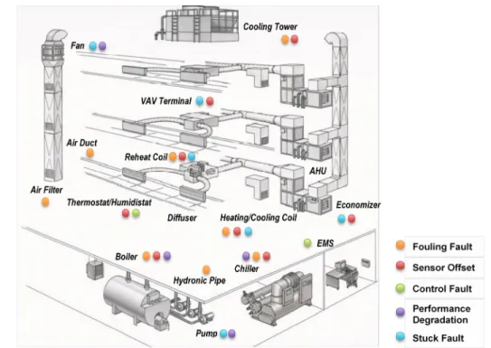
Heating, ventilating, and air conditioning (HVAC) system operations in buildings represent a significant potential for reducing energy use in buildings by improving energy efficiency, indoor air quality, and comfort levels. However, most buildings, especially those embedded with complex building energy systems, have various degrees and types of operational problems. It is reported that the number of maintenance requests for building energy systems have increased exponentially throughout the past decades, indicating an increase in building operational faults [3]. Typical operational faults may come from improper installation, equipment degradation, sensor offset or failures, or control logic problems. They can be grouped into several categories, including: (1) control fault, (2) sensor offset, (3) equipment performance degradation, (4) fouling fault, (5) stuck fault, and (6) others [4,5]. Figure 1 depicts a number of common potential faults in a typical variable air volume (VAV) system with a central plant.

Figure 1 Potential HVAC operational faults in a typical VAV system in a central plant

HVAC operational faults may lead to a considerable discrepancy between actual HVAC operation performance and design expectations [6–9]. It is estimated that poorly maintained and improperly controlled HVAC equipment is responsible for 15% to 30% of energy consumption in commercial

buildings [5]. A series of questionnaire surveys and interviews conducted by Au-Yong, et al., show the significant influence of poor HVAC operation on occupant comfort, and a number of maintenance factors are identified that are significantly correlated with the occupants' satisfaction [10].

Modeling and simulating HVAC operational faults can lead to greater understanding by quantifying the impact of the faults on building energy use and occupant comfort. Modeling and simulation allows for an estimation of the severity of common faults and, thus, supports decision making about timely fault corrections—which can then enable efficient system operation, improve indoor thermal comfort, reduce equipment downtime, and prolong equipment service life [11–13]. It can also support commissioning efforts by providing estimates for potential energy/cost savings that could be achieved by fixing the faults during retro-commissioning. Quantified information on the impacts and priorities of various coexisting operational faults can be provided to the commissioners or the building management system, resulting in more reasonable and reliable commissioning decisions, especially when budget and staff resources are limited [13]. Moreover, modeling operational faults is critical to achieving more reliable energy model calibrations when most energy models for existing buildings assume ideal conditions without any operational problems. This ability to estimate the severity of common faults is expected to improve the accuracy and transparency of the calibrated model, therefore increasing the analysis accuracy of different retrofit measures [14,15].

A variety of fault detection and diagnosis (FDD) tools have been developed with various approaches, focusing on identifying and analyzing the HVAC operational problems. Cheung and Braun developed the fault models for a variety of typical building energy system equipment with three modeling techniques: empirical modeling, semi-empirical modeling, and physical modeling [4,16]. Radhakrishnana, et al. investigated the various constraints of HVAC scheduling and proposed a novel, token-based distributed control/scheduling approach that can account for varying indoor environment and occupant conditions [17]. Zhao, et al. proposed a pattern recognition-based method to detect and diagnose faults in chiller operations, using a one-class classification algorithm [18]. Li, et al. also investigated the chiller operational problems, but with a two-stage, data-driven approach based on the linear discriminant analysis [19]. Cai, et al. developed a novel method to analyze the faults of the ground-source heat pump. Cai’s model achieves multi-source information fusion-based fault diagnosis by deriving Bayesian networks based on sensor data [20]. Han, et al. proposed an automated fault detection and diagnosis strategy for vapor-compression refrigeration systems, combining the principle component analysis feature extraction technology and the multiclass support vector machine classification algorithm [21]. The operational faults of several other major HVAC components have also been investigated, such as air handle unit (AHU) [22–24], heat exchanger [25], and fan coil unit [26].

strategies of HVAC systems, however, research on the impacts of HVAC operational faults is still insufficient. Most fault-related research focuses on the component or subsystem performance rather than the whole-building performance and therefore cannot predict the overall impacts of the faults at the building level. The synchronized effect between simultaneous faults occurring in multiple components cannot be effectively addressed by existing approaches. Moreover, the current fault analysis methods are usually designed for specific HVAC systems employed in particular case buildings. This leads to significant challenges in applying the approaches to buildings with different system types or configurations.

Whole-building performance simulation can be a powerful tool in addressing the aforementioned fault analysis limitations. Techniques for building information modeling and whole-building energy simulation have improved significantly in the past two decades with the help of great advances in computational power and algorithms. These techniques have been widely used in the current architecture, engineering, and construction (AEC) industry throughout the world to support building physics research and actual new/retrofitting building design, operation, and management [27–29].

This paper introduces the methodology of modeling and simulating operational faults using EnergyPlus, a comprehensive whole-building performance simulation program. It outlines the challenges of operational fault modeling using building simulation programs, and compares three approaches to simulating operational faults using EnergyPlus. This paper also introduces the latest development of native fault objects within EnergyPlus, as well as future development plans to further improve the fault-modeling capability of EnergyPlus. The fault-fault-modeling feature in EnergyPlus fills in the gap of building performance simulation to improve the accuracy of modeling existing buildings where operational faults are common and have significant impacts on building performance.

2

Challenges of Building Operational Faults Modeling and Analysis

As building energy system configuration and control becomes increasingly complex, it presents several challenges for modeling and analyzing HVAC operational faults at the building level. In general, the following issues need to be taken into account and well addressed in a whole-building performance simulation to model and quantify the overall impacts of operational faults on the building.

Firstly, the building energy system can be a sophisticated system with numerous interrelated equipment components that may present complex interrelation and coupling effects. Building operational faults can occur at different levels: component, subsystem, system, or even building level. A fault at any of these levels can further affect the operations of many other related components, and therefore, makes it difficult to understand the relationship between causes and effects and to quantify the overall impacts on the whole-building energy performance [30,31]. For example, the degradation of fans may affect the air

side of the system by reducing the supply airflow or increasing fan power. It may also affect the heat transfer performance of coils and its energy consumption, thus further affecting the water side performance of the system.

Secondly, the operational faults may present diverse impacts on different aspects of the building performance. For instance, a positive offset of the thermostat (i.e., the zone air temperature reading is higher than the actual value) can generate different influence on both the energy consumption and thermal comfort during different seasonal periods. During the heating seasons, it reduces the heating energy consumption by maintaining the room temperature at lower levels, but, meanwhile, it deteriorates the indoor thermal comfort conditions. During the cooling seasons, energy consumption increases, and over-cooling may present. Investigations of these diverse impacts are essential to understanding overall fault impacts.

Thirdly, one particular fault may present very different operational characteristics and needs to be handled with a different approach. Taking the temperature sensor offset as an example, it can be: (1) a static fault, if the offset is a constant value throughout the analysis period, (2) an abrupt fault, if the offset arises suddenly during the analysis period and stays at a constant level after occurrence, (3) a degradation fault, if the sensor offset drifts over time. These different cases need to be carefully distinguished and modeled using various methods which may use different features of the modeling tools. Some current research assumes the abrupt and degradation fault to be static because of the limitations of modeling tool capacity [32], but this may oversimplify the problem.

Fourthly, the fault model design and implementation needs to take into account the characteristics of existing component models in the building energy simulation programs. Fault models are usually built upon and applied to specific existing component models. For instance, the condenser supply water sensor offset fault model is applied to the cooling tower model, because the fault leads to different cooling tower behaviors during faulty operation. The component model can be either physics-based or empirical. Physics-based component models have more operational parameters defined in the algorithm that can be directly manipulated by the fault model. This provides more flexibility for the fault model design and implementation. By contrast, an empirical component model is mainly based on the performance curves instead of first-principle physics, and therefore provides limited flexibility to apply the fault model. In this case, the fault model needs to be well designed to make use of the component model features and balance the model applicability and accuracy.

Finally, fault modeling and simulation tools should take into account various modes of HVAC system operations. For example, many faults may present significant impacts during normal modes but little or no impacts in free cooling modes. Operational faults may also need to be handled separately with different building simulation cases. For example, the thermostat or humidistat offset fault should only be

introduced during the normal weather simulation case, but not the sizing case where maximum loads are calculated to determine the capacity of HVAC equipment. Since the offsets are unknown during the design phase, they should not affect the sizing of the system. Therefore, fault-modeling tools should have flexible and capable modeling capacities.

3

Fault-modeling Approaches using EnergyPlus

Compared with the fault detection and diagnosis methods developed based on specific reduced-order models, the fault-modeling approach presented in this paper has remarkable advantages. This approach makes use of the well-established building modeling and simulation capabilities of EnergyPlus, which enables it to address the challenges discussed above.

EnergyPlus is a whole-building performance simulation tool that can be used to investigate operational faults. It is the flagship building simulation engine supported by the US DOE. It can model heating, ventilation, cooling, lighting, water use, renewable energy generation, and other building energy flows by including many innovative simulation capabilities. Capabilities can include sub-hourly time-steps, modular systems, and plant systems integrated with heat balance-based zone simulation, multi-zone air flow, thermal comfort, water use, natural ventilation, renewable energy systems, and user customizable energy management systems. EnergyPlus can also handle the high-order building energy models containing detailed information about the functional and physical characteristics of the buildings, and can perform co-simulations of large numbers of subroutines to obtain more accurate estimations on the whole-building performance [27,33]. Each release of EnergyPlus is extensively tested using more than four hundred example files; test cases are defined in ASHRAE Standard 140. EnergyPlus is a powerful tool that supports building professionals, scientists, and engineers in optimizing building design and operations, and thus helps to reduce energy and water consumption [27]. Although EnergyPlus has been primarily used in the building design phase, it has capabilities to model and simulate HVAC operational faults in the following three approaches.

The first approach is direct modeling in the EnergyPlus input data files (IDF). The advantage of this approach is easy implementation. Users can change the input parameters or performance curves to describe the faulty operations, run the IDF file in a normal way, and then compare the results with the fault-free cases. However, users can only modify existing input parameters, which are not specifically designed for fault modeling. Also, this approach is usually limited to addressing static faults such as outdoor air (OA) damper leakage or simplified operational issues such as chiller fouling described by an empirical degradation factor [11]. It can rarely handle complex fault models, especially those requiring sophisticated physical calculations. Furthermore, users need to be careful to set up the fault models that are do not affect the sizing period in the simulation. Many auto-sizing features of EnergyPlus may need to

be avoided as a tradeoff of direct modeling of operational faults.

The second approach is to use energy management system (EMS), an advanced feature of EnergyPlus. It is a scripting language that allows the development of customized supervisory controls to override selected aspects of EnergyPlus modeling [34]. Compared with a direct modeling approach, EMS provides more flexibility to the user to design or overwrite algorithms in EnergyPlus within the specified aspects of current EMS capability, and is more powerful in handling complex fault models such as dirty filters with increasing pressure drops during simulation periods. This approach, however, only offers users limited access to a pre-selected set of parameters, i.e., EMS sensor and actuator set. It cannot address the fault models requiring parameters out of the set. In addition, users need to program specific logic to describe the fault model for a particular building system. This makes it laborious and inflexible when transferring the fault model to other building models with different system configurations. Moreover, EMS is an advanced feature designed for EnergyPlus professional users. It requires computer programming skills as well as a deep understanding of the connections between the faulty component and related objects. This may limit its adoption by the average building energy modelers and practitioners.

The third approach is to use native fault objects within EnergyPlus. This approach has remarkable advantages in terms of usability, capability, flexibility, and transferability. With this approach, users have full access to all the EnergyPlus parameters in source codes; the complexity of the fault models is no longer a problem. Using this approach, developers can implement substantial generic physical logics in the source codes (e.g., the algorithm calculating the impacts of dirty air filter pressure drop increase on the airflow delivering the performance of various types of fans). Therefore, users only need to provide the fault information required in the IDD (Input Data Dictionary of EnergyPlus) without worrying about the description of its calculation logic. This greatly reduces modeling burdens for users compared with the EMS approach. Therefore, this approach can be more widely adopted by both practitioners and energy modeling experts. Moreover, the native fault objects for various building system configurations are fairly generic, making the fault modeling more transferable from one building model to the other. Note that this approach is easy and user friendly, but it requires a considerable amount of work from the EnergyPlus developers to design and implement the objects. As described in the following section, current EnergyPlus V8.6 can address four common fault types. More fault types will be addressed in future EnergyPlus releases.

4

Native Fault Objects within EnergyPlus

A review of operational faults in buildings was carried out, and a number of common HVAC equipment faults were identified in previous studies [4,5]. These faults were then ranked according to

both the complexity of implementation and the severity of associated energy penalty. A group of fault models was added to EnergyPlus starting with Version 8.1. Several faults can be implemented by adding new fields to the existing EnergyPlus IDD objects, such as the “air damper stuck” fault. However, this approach is not preferred because such inputs are only needed when modeling faults and can be unnecessary burdens for modeling normal fault-free cases. For easy code maintenance and usability, a group of native fault objects were created. These new objects have a generic design in common, pointing to one or a list of existing equipment objects that have faults, and using one schedule describing the availability or applicability of faults and another schedule describing the severity of faults.

Based on the ranking, four types of occurring faults have been implemented via native objects in EnergyPlus version 8.6, including:

(1) Sensor faults with air economizers, (2) Thermostat/humidistat offset,

(3) Heating and cooling coil fouling, and (4) Dirty air filters.

The symptoms and modeling approaches of these operational faults are introduced in detail in the sections below. All of the fault models are based on existing EnergyPlus models that have been validated via extensive analytical and comparative tests [35–37]. In the fault model development and implementation, comparative data analysis, using detailed EnergyPlus time-step reports, is performed at the equipment component level for validation purposes. Extreme cases are also developed to verify the fault objects. Taking the economizer OA temperature sensor fault, for example, the case with fault offset value of 0°C is verified with the fault-free case, and the case with extremely large offset (e.g., 20°C) is verified with the case without an economizer.

Collecting model inputs is an essential step for fault modeling and simulation. Some inputs can be easily obtained by site commissioning, for example, the thermostat offset. Some information can be obtained from manufacturers, such as the fan curve used to estimate the airflow decrease due to air filter fouling. For some others, such as the U-value decrease due to fouling at coil or cooling tower, it may be challenging to perform accurate measurements. In such cases, inputs can be estimated based on rules-of-thumb or literature review.

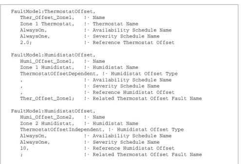
Figure 2 shows an example of IDF codes for modeling the thermostat/humidistat offset faults in two thermal zones. FaultModel:ThermostatOffset and FaultModel:HumidistatOffsetZone are the objects designed to collect the thermostat/humidistat offset faults information, respectively. Zone 1 has a fault of humidistat offset, which is described in Humi_Offset_Zone1. The fault points to the zone humidistat named Zone 1 Humidistat, on which the fault is applied. Also, note that the fault is caused by a linked thermostat, so a corresponding thermostat offset fault named Ther_Offset_Zone1 is created in the model.

By contrast, the fault of humidistat offset in Zone 2, as described by Humi_Offset_Zone2, is thermostat independent and therefore does not point to a corresponding thermostat offset.

Figure 2 Example of IDF codes for the thermostat/humidistat offset fault models

These fault models within EnergyPlus can handle different types of faults, including static, abrupt, and degradation faults. This is achieved by defining two schedules in the fault object, i.e., availability schedule and severity schedule. The former can determine whether the fault is applicable or not, while the latter can define a time-dependent multiplier to the reference thermostat offset value.

4.2 Economizer Sensor Offset

Background:

An air-side economizer is a type of mechanical device integrated into an air handling system. It can introduce a specific amount of outside air as a means of cooling the indoor space when the outside air is cooler (in terms of dry-bulb temperature or enthalpy of the air) than the recirculated air. It can reduce cooling energy use and potentially improve the indoor air quality by using more OA in locations with good OA quality. Therefore air-side economizers are widely used in various regions especially those with cold and temperate climates. A number of temperature and humidity sensors are implemented in the economizer to ensure its proper control and operations.

Symptom:

The sensor readings deviate from the actual air conditions, which leads to inappropriate operations of the air economizer and thus undesired resulting indoor conditions.

There are many sensors installed in the economizer to provide essential information for its proper operations. These sensors may be of different types depending on the economizer type, including temperature sensor, humidity sensor, enthalpy sensor, and pressure sensor. In the current EnergyPlus, a number of objects are designed to describe the fault of different types of sensors at various economizer locations. For example, many economizers operate based on the dynamic temperature levels of the OA and RA, which are measured by two temperature sensors separately. If there is an offset for the OA senosr, the object of FaultModel:TemperatureSensorOffset:OutdoorAir can be used to describe the problem.

The effect of an offset in a sensor whose sole use is for calculation of the difference between the set-point and actual air condition can be modeled as an equal and opposite offset in the set-point:

Tf = Tff ± ΔT (1)

RHf = RHff ± ΔRH (2)

hf = hff ± Δh (3)

Where

T/RH/hf temperature/humidity/enthalpy value for the faulty sensor case

T/RH/hff temperature/humidity/enthalpy value in the fault-free case (design value)

ΔT/RH/hdifference between faulty sensor reading and the actual value

Note that the economizer sensor set-points are related with two major processes within EnergyPlus: one is the design load calculations and HVAC system sizing and the other is the HVAC system operations. Only the latter is affected by the economizer sensor offset, while the former is not. Therefore, the two processes are addressed separately in the development of the sensor offset fault model.

4.3 Thermostat/Humidistat Offset

Background:

The thermostat/humidistat is a key control unit for HVAC systems. It is used to sense the temperature/humidity of air in a system or space so that the air condition is maintained near a desired level. As an electronic device, the thermostat/humidistat needs to be calibrated periodically to ensure its accuracy.

Symptom:

The zone air T/RH readings deviate from the actual indoor air T/RH levels due to thermostat/humidistat offset, leading to inappropriate operations of the heating/cooling/humidifying/dehumidifying equipment. Approach:

The effect of an offset in a thermostat/humidistat whose sole use is for the calculation of the difference between the set-points and the design air conditions can be modeled as an equal and opposite offset in the thermostat/humidistat:

Tstat,f = Tstat,ff ± ΔTstat (4)

RHstat,f = RHstat,ff ± ΔRHstat (5)

Where

Tstat,f/RHstat,f thermostat/humidistat value in faulty case

Tstat,ff/RHstat,ff thermostat/humidistat value in the fault-free case (design value)

ΔTstat/ΔRHstat difference between thermostat/humidistat reading and the actual zone T/RH

Note that the humidistat offset faults can be divided into two types: thermostat fault dependent and independent. The thermostat-independent humidistat directly measures the relative humidity of the air without calculations that use air temperature. For example, the nylon ribbon humidistat is constructed according to the hygroscopic nylon film technology, which estimates the relative humidity level by measuring the elongation of a nylon ribbon as a function of relative humidity. By contrast, the thermostat-dependent humidistat obtains the relative humidity level based on the measured temperature level. For example, the electronic capacitive humidity sensor is designed based on the capacitive effect. It employs a capacitor formed by a hygroscopic dielectric material and a pair of electrodes. The capacitance is directly measured to indicate the level of water vapor pressure, and then the relative humidity level is further calculated as a function of the ambient temperature and humidity ratio.

These two types of the faults need to be addressed differently. For the humidistat that is independent of the thermostat, ΔRH can be simply described by a pre-defined schedule. For the humidistat offset that is caused by the thermostat offset, however, ΔRH is related with both the thermostat offset level as well as the indoor air conditions which are dynamic, and therefore cannot be described with a pre-defined schedule. In this case, the humidistat offset level is calculated at each time step.

ΔRHstat = RHstat,ff - f(Treal, Wf) (6)

Where

Treal real-time temperature of the indoor air (real value), °C

Wf humidity ratio corresponding to Treal±ΔT and RHstat,ff, kgWater/kgDryAir

The thermostat offset fault is described in the FaultModel:ThermostatOffset object and further applies to the following objects in EnergyPlus:

(2) ZoneControl:Thermostat:TemperatureAndHumidity (for temperature control considering zone air humidity conditions),

(3) ZoneControl:Thermostat:OperativeTemperature (for operative temperature based control).

The humidistat offset is described in the FaultModel:HumidistatOffset object and further applies to

ZoneControl:Humidistat (for traditional air relative humidity control).

4.4 Fouling Coils

Background:

As the most widely used type of heat exchangers, heating and cooling coils may present fouling faults. This usually occurs at the water side of the coil when deposits get clogged due to poor water quality and treatment.

Symptom:

Reduced overall heat transfer coefficient (UA) causes reduced coil capacity, resulting in unmet loads and/or increased water flow rate and decreased water side temperature difference (“low ΔT” syndrome). Approach:

The fault model is described in the FaultModel:Fouling:Coil object and further applies to the water coils described by:

(1) Coil:Heating:Water (for water-based heating coils), (2) Coil:Cooling:Water (for water-based cooling coils).

The model allows the user to describe the fouling information in either of the two methods:

FouledUARated, or FoulingFactor. In the FouledUARated method, the user specifies the value of UAfouled

directly. In the FoulingFactor method, the user specifies air/water side fouling factor, and the UAfouled

value is further calculated via:

UAf = [(UAair)-1 + Rfoul + (UAwater-1)]-1 (7)

Where

UAair heat transfer coefficient of the coil on the air side, W/K

UAfouled overall heat transfer coefficient of the fouled coil, W/K

UAwater heat transfer coefficient of the coil on the water side, W/K

Rfoul fouling factor, K/W

Rfoulis determined by:

Rfoul = rair/Aair + rwater/Awater (8)

rair Air side fouling factor, m2K/W

rwater Water side fouling factor, m2K/W

Aair Air side coil surface area, m2

Awater Water side coil surface area, m2

The pressure drop associated with the fouling is ignored in this implementation, because its impact is usually not significant compared to its impact on the heat transfer performance of the coil.

4.5 Dirty Air Filters

Background:

Air filters are implemented at the OA inlets or other duct locations to reduce the amount of particulate matter or contaminants that are brought into the air system. The dust, debris, or other blockages can gradually accumulate at the air filter during its operations.

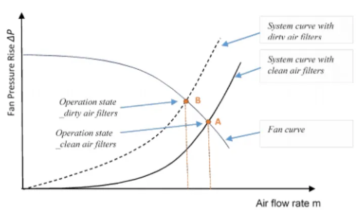
Symptom:

Increased air loop system resistance resulting in a different system curve. This directly affects the operation of corresponding fans. More specifically, it may lead to an increase in the fan pressure rise, fan energy consumption, and/or the enthalpy of the fan outlet air. It may also lead to a reduction in the airflow rate and thus affects the performance of other system components (e.g., heat transfer performance of heating/cooling coils).

Approach:

The dirty air filter fault is described in the FaultModel:Fouling:AirFilter object and further applies to existing fan objects that describe the normal operational behavior of the fans. The fault object introduces a curve to describe the relationship between fan pressure rise and air flow rate, as well as a schedule to describe the dynamic variations of the fan pressure rise due to the air filter fouling. More specifically, the fault model applies to the following fan types represented in EnergyPlus objects:

(1) Fan:ConstantVolume (for the common constant air volume fan),

(2) Fan:OnOff (for the constant air volume fan that is intended to cycle on and off), (3) Fan:VariableVolume (for the variable air volume fan).

The operating performance of a fan is related to a number of factors, including the fan types, system design, and operating conditions. In general, there are three possible situations to be addressed in modeling dirty air filters as described below. The developed fault model is able to handle these situations with a fan curve and pressure increase schedule provided by the user.

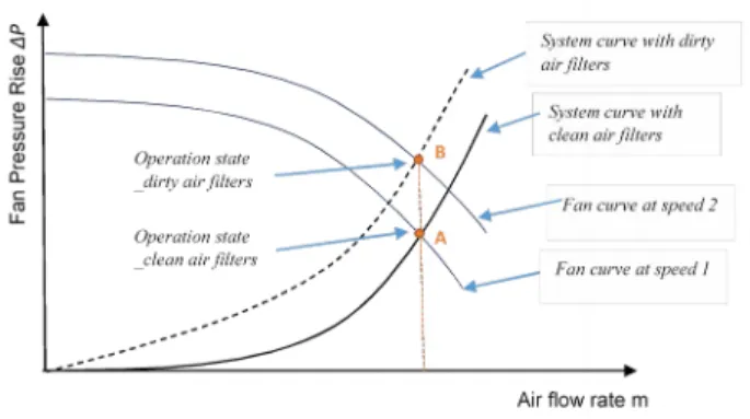
In this case, the fan operation state changes from point A (intersection of the fan curve corresponding to a lower speed and the system curve with clean filters) to point B (intersection of the fan curve corresponding to a higher speed and the system curve with dirty filters), as shown in Figure 3. Point B corresponds to a higher fan pressure rise than Point A, and the same air flow rate.

Figure 3 Effect of dirty air filter on variable speed fan operation – flow rate maintained

The required airflow rate m can be maintained while the fan pressure rise ∆P is increased to ∆Pdf. This

leads to higher fan power (Qtot) and higher power entering the air (Qtoair), and thus changes the specific

enthalpies of the fan outlet air stream (hout).

fflow,df = m / mdesign,df (9)

fpl,df = c1 + c2×fflow,df + c3×fflow,df2 + c4×fflow,df3 + c5×fflow,df4 (10)

Qtot,df = fpl,df × mdesign,df × ∆Pdf / (etot ×ρair ) (11)

Qshaft,df = emotor ×Qtot, df (12)

Qtoair,df = Qshaft,df +( Qtot,df - Qshaft,df) ×fmotortoair (13)

hout,df = hin + Qtoair,df / m (14)

Where

emotor motor efficiency

fflow flow fraction or part-load ratio

fpl part load factor

m air mass flow, kg/s

Qtot fan power, W

Qtoair power entering the air, W

Qshaft fan shaft power, W

∆P fan pressure increase, Pa

design for the parameters in the design condition df for the parameters in the dirty filter case.

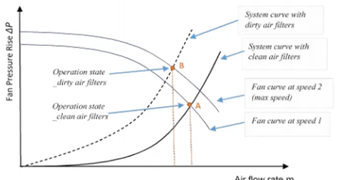
In this case, the fan operation state changes from point A (intersection of the fan curve corresponding to a lower speed and the system curve with clean filters) to point B (intersection of the fan curve corresponding to a higher speed and the system curve with dirty filters), as shown in Figure 4. Point B corresponds to a higher fan pressure rise and a lower air flow rate than Point A.

Figure 4 Effect of dirty air filter on variable speed fan operation – air flow rate reduced

The airflow rate m is reduced to mdf while the fan design pressure rise ∆P is increased to ∆Pdf. Similarly to

the case (a), the fan power (Qtot), the power entering the air (Qtoair), and the specific enthalpies of the fan

outlet air stream (hout) are all affected. Additionally, the flow fraction fflow becomes 1 in case (b).

fflow,df = 1 (1

5)

fpl,df = c1 + c2×fflow,df + c3×fflow,df2 + c4×fflow,df3 + c5×fflow,df4 (1

6)

Qtot,df = fpl,df × mdesign,df × ∆Pdf / (etot × ρair ) (1

7)

Qshaft,df = emotor ×Qtot, df (1

8)

Qtoair,df = Qshaft,df +( Qtot,df - Qshaft,df) ×fmotortoair (1

9)

hout,df = hin + Qtoair,df / m design,df (2

0)

(c) The constant speed fan cannot maintain thedesign airflow rate.

In this case, the fan operation state changes from point A (intersection of the fan curve and the system curve with clean filters) to point B (intersection of the fan curve and the system curve with dirty filters), as shown in Figure 5. Point B corresponds to a higher fan pressure rise and a lower air flow rate than Point A.

Figure 5 Effect of dirty air filter on constant speed fan operation

Similarly to the case (b), the airflow rate m is reduced to mdf while the fan pressure rise ∆P is increased to

∆Pdf. This results in variations of the fan power (Qtot), the power entering the air (Qtoair), and the specific

enthalpies of the fan outlet air stream (hout).

Qtot,df = mdf × ∆Pdf / ( etot ×ρair ) (2

1)

Qshaft,df = emotor × Qtot, df (2

2)

Qtoair,df = Qshaft,df +( Qtot,df - Qshaft,df )×fmotortoair (2

3)

hout = hin + Qtoair,df / mdf (2

4)

5

Impacts of Operational Faults: A Case Study

As an example, EnergyPlus version 8.6 is used to investigate the impacts of the aforementioned operational faults in a typical small-size office building across several representative U.S. climate zones as shown in Table 1. The study case is a single-story rectangular building (30m × 15m) that includes four exterior and one interior conditioned zones (2.4m high) and a return plenum (0.6m high). The walls are made of three material layers: a wood shingle over plywood, a R11 insulation, and a gypsum board. The roof is a gravel built-up roof with R-3 mineral board insulation and plywood sheathing. The windows are of various single and double pane construction with 3mm and 6mm glass and either 6mm or 13mm argon or air gap. The window-to-wall-ratio is 0.29. The south wall and door have overhangs. The building has a standard VAV system with an outside air economizer, a central chilled water cooling coil, a main hot water heating coil, and multiple hot water reheating coils. The central plant includes a single hot water boiler, an electric compression chiller with a water-cooled condenser, an electric steam humidifier, and a cooling tower. The capacities of these equipment are automatically determined using the equipment

autosizing feature of EnergyPlus based on the typical meteorological year weather data of the studied cities. The system controls the high relative humidity set-point of 70% with the chilled water coil and low humidity set-point of 30% with the electric steam humidifier. The model is simulated for the whole year with a time step of 15 minutes. More details of the model can be found in the example file of

5ZoneWaterCooled_MultiZoneMinMaxRHControl.idf in the official EnergyPlus releases [33]. The annual building heating and cooling energy consumption is used to evaluate the fault impacts on the building energy efficiency, and the value of set-point unmet hours with a default setting of 0.5°C is used to estimate the fault impacts on occupant thermal comfort.

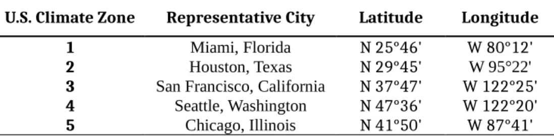
Table 1 Representative cities in the case study

U.S. Climate Zone Representative City Latitude Longitude

1 Miami, Florida N 25°46' W 80°12'

2 Houston, Texas N 29°45' W 95°22'

3 San Francisco, California N 37°47' W 122°25'

4 Seattle, Washington N 47°36' W 122°20'

5 Chicago, Illinois N 41°50' W 87°41'

5.1 Impact of Economizer Sensor Offset

An economizer OA sensor is more likely to have an offset due to its exposure to the outdoor conditions. The following two cases are modeled and simulated to estimate the impacts of economizer OA sensor offset, using the native fault objects of FaultModel:TemperatureSensorOffset:OutdoorAir:

- Case 1: economizer OA sensor with an offset of -2°C - Case 2: economizer OA sensor with an offset of -4°C

The type of the economizer in the case building is DifferentialDryBulb, meaning that the economizer will increase the OA flow rate when there is a cooling load and the sensed OA temperature is below the zone return air (RA) temperature. The OA sensor offset fault can affect the correct operation of the economizer. More specifically, the sensor with a negative offset reads a temperature that is lower than the real true value, so the economizer opens the OA damper even when the OA temperature is higher than the RA temperature. The injection of hot OA into the building by the faulty sensor and the opened damper increases the cooling load for the coil and therefore increase the cooling energy of the building.

The comparisons of the cooling energy consumption are provided in Figure 6. As it can be seen in the figure, Case 1 leads to the cooling energy consumption increase of 0.8%—5.8% compared to the fault-free case, while Case 2 increases the cooling energy consumption by 2.1%—13.6%. Because the fault does not affect supply air conditions as long as the cooling coil capacity is sufficient, indoor thermal comfort is usually not affected. The heating energy of the building is also not impacted.

Figure 6 Impact of economizer outdoor air sensor offset on building cooling energy consumption 5.2 Impact of Thermostat/Humidistat Offset

The following two cases are modeled and simulated to estimate the impacts of thermostat/humidistat offset faults, using the native fault objects of FaultModel:ThermostatOffset and

FaultModel:HumidistatOffset:

- Case 1: humidistat offset caused by dependent thermostat with an offset of 1°C - Case 2: humidistat offset caused by dependent thermostat with an offset of -1°C

In the study case, the humidistat offset fault is caused by the thermostat offset fault. These two types of faults present a coupling effect to the HVAC system control. Also, the humidistat offset is a function of the constant thermostat offset as well as the dynamic indoor air conditions. These make it complex to estimate the fault impacts on system operations, either qualitatively or quantitatively.

The comparisons of the energy consumption and occupant comfort are depicted in Figure 7 and Figure 8, respectively. As can be observed in Figure 7, both of the faulty cases lead to a remarkable influence on heating and cooling energy consumption in all of the investigated cities. Case 1 leads to a cooling and heating energy reduction of 12.47%—28.19% compared to the fault-free case, while Case 2 increases the cooling and heating energy consumption by 19.07%—34.24%. Figure 8 shows that the fault also dramatically changes the set-point unmet hours during heating and cooling periods, indicating significant impacts on occupancy thermal comfort levels.

Figure 7 Impact of the integrated thermostat/humidistat offset faults on the building cooling and heating energy consumption

Figure 8 Impact of the integrated thermostat/humidistat offset faults on the indoor thermal comfort 5.3 Impact of Fouling Coils

The case building implements a main hot water heating coil and multiple hot water reheating coils, all of which are modeled via Coil:Heating:Water. Fouling can significantly impact the heat transfer performance of the coil, especially when the water quality is poor. The following two cases are modeled and simulated to estimate the impacts of fouling on heating coils in the building:

- Case 1: heating coil fouling leads to a 25% reduction of the coil overall UA (U-factor times area) value

- Case 2: heating coil fouling leads to a 50% reduction of the coil overall UA value

The fouling of the coil presents extra heat transfer resistance and decreases the coil capacities. This can lead to insufficient heating of the supply air, and then further affect indoor comfort levels. Figure 9 displays the impact of coil fouling in the study case. The figure shows that the fault leads to a dramatic increase of unmet heating hours for all the investigated cities, indicating significant impacts on occupancy thermal comfort. Note that the fault does not necessarily increase the heating energy of the building, because of the decrease of the heating coil capacity caused by the fouling.

Figure 9 Impact of coil fouling on indoor thermal comfort 5.4 Impact of Dirty Air Filters

The following two cases are modeled and simulated to estimate the impacts of dirty air filters in the case building, using the native fault objects of FaultModel:Fouling:AirFilter. Note that a fan curve also needs to be provided in the fault modeling to calculate the airflow rate decrease due to the increase of fan pressure drop, and the curve needs to cover the design point specified in the fan modeling.

- Case 1: air filter fouling leads to a 10% increase of the fan pressure rise at the rated condition - Case 2: air filter fouling leads to a 20% increase of the fan pressure rise at the rated condition

Figure 10 Pressure-flowrate curve of the variable speed fan at the maximum speed

The study case implements a variable speed fan for the air system, on which the fault is applied. Figure 10 depicts the pressure-flowrate curve of the fan at the maximum speed. In both the (a) and (b) situations described in section 4.5, the fan flow fraction at the faulty case is higher than the fault-free case which leads to increased fan energy consumption.

Figure 11 plots the comparison of fan energy consumption in the case building across the investigated cities. As can be found in the figure, both faulty cases lead to a significant increase in the fan energy consumption. Case 1 leads to a fan energy increase of 4.32%—5.30% compared to the fault-free case, while Case 2 increases the fan energy consumption by 7.41%—9.52%. Since the variable speed fan can usually maintain the airflow rate by shifting to a higher speed, heating and cooling energy consumption, as well as indoor thermal comfort, is not significantly affected in the study case.

Figure 11 Impact of the air filter fouling on fan energy consumption

6

Future Fault Development Plan

With the U.S. DOE’s high priority focus on the retrofit and operations improvement of existing buildings, EnergyPlus capabilities need to be extended to model existing buildings, including faulty operational faults. A number of new fault objects are under development, focusing on the operational faults in the central plant systems. These fault models are available in the EnergyPlus version 8.7 release, including:

(1) Boiler fouling,

(2) Cooling tower scaling, (3) Chiller fouling,

(4) Chiller water temperature sensor offset, (5) Coil supply air temperature sensor offset, (6) Condenser water temperature sensor offset.

Note that the fault models will be deployed to the corresponding equipment component models that already exist in EnergyPlus. Therefore, they need to be designed particularly to take into account the characteristics of the equipment models. In general, a more physics-based equipment model can offer more flexibility to the development of the corresponding fault model, since it allows the manipulation of more operational parameters. For the equipment models that are mainly based on empirical curves, however, there will be less flexibility due to limited access to operational parameters. Design and implementation of the plant equipment fault models must address ways to better use existing equipment model features and ways to handle various levels of constraints.

7

Conclusions

This study presents the novel development of modeling HVAC operational faults in EnergyPlus, which enables EnergyPlus simulation models to capture operational faults that are common in existing buildings, quantify the impacts of faults on building energy use and occupant thermal comfort, and thus support the decision making of timely fault correction during normal building maintenance or the commissioning process. The case study demonstrated that the faults have significant impacts on the energy performance of HVAC systems as well as occupant thermal comfort.

The study contributes to the new body of knowledge by adding a new category of fault-modeling feature in EnergyPlus to improve the accuracy of modeling existing buildings, which is critical for energy retrofit or commissioning projects targeting reduction of energy use in buildings and improvement of occupant comfort. Future work includes the development of additional faults in EnergyPlus to cover

operational faults in central plant systems.

Acknowledgment

This work was supported by the Assistant Secretary for Energy Efficiency and Renewable Energy of the U.S. DOE under Contract No. DE-AC02-05CH11231. The authors thank Jason Glazer, Howard Cheung, Jim Braun, Michael J. Witte, Lixing Gu, and Daniel Macumber for their constructive suggestions and discussions during the development of these fault models as new features for EnergyPlus.

References

[1] DOE, Buildings Energy Data Book, Washington D.C., 2011.

[2] EPC, Directive 2010/31/EU of the European Parliament and of the Council of 19 May 2010 on the energy performance of buildings, Off. J. Eur. Union. 153 (2010) 13–35.

[3] D. Cotts, Roperathy, R. Payant, The Facility Management Handbook, 3rd ed., Amarican Management Association, 2010.

[4] H. Cheung, J.E. Braun, Development of Fault Models for Hybrid Fault Detection and Diagnostics Algorithm, National Renewable Energy Laboratory, Boulder, CO, 2015.

[5] Mangesh Basarkar, X. Pang, L. Wang, P. Haves, T. Hong, Modeling and simulation of HVAC faults in EnergyPlus, IBPSA Build. Simul. (2013) 14–16. http://escholarship.org/uc/item/9ps43482.pdf. [6] N. Djuric, V. Novakovic, Review of possibilities and necessities for building lifetime commissioning,

Renew. Sustain. Energy Rev. 13 (2009) 486–492. doi:10.1016/j.rser.2007.11.007.

[7] O.T. Karaguzel, R. Zhang, K.P. Lam, Coupling of whole-building energy simulation and multi-dimensional numerical optimization for minimizing the life cycle costs of office buildings, Build. Simul. 7 (2014) 111– 121. doi:10.1007/s12273-013-0128-5.

[8] R. Zhang, T. Hong, Modeling and Simulation of Operational Faults of HVAC Systems using EnergyPlus, in: ASHRAE IBPSA-USA SimBuild 2016 Perform. Model. Conf., Salt Lake City, UT, 2016.

[9] S. Wang, J. Cui, Sensor-fault detection, diagnosis and estimation for centrifugal chiller systems using principal-component analysis method, Appl. Energy. 82 (2005) 197–213.

doi:10.1016/j.apenergy.2004.11.002.

[10] C.P. Au-Yong, A.S. Ali, F. Ahmad, Improving occupants’ satisfaction with effective maintenance management of HVAC system in office buildings, Autom. Constr. 43 (2014) 31–37.

doi:10.1016/j.autcon.2014.03.013.

[11] L. Wang, T. Hong, Modeling and Simulation of HVAC Faulty Operation and Performance Degradation due to Maintenance Issues, ASim 2012 - 1st Asia Conf. Internatinal Build. Perform. Simul. Assoc. DE-AC02-05

(2013).

[12] M.C. Comstock, J.E. Braun, E.A. Groll, A survey of common faults for chillers, ASHRAE Trans. 108 (2002) 819–825.

[13] L. Wang, S. Greenberg, J. Fiegel, A. Rubalcava, S. Earni, X. Pang, R. Yin, S. Woodworth, J. Hernandez-Maldonado, Monitoring-based HVAC commissioning of an existing office building for energy efficiency, Appl. Energy. 102 (2013) 1382–1390. doi:10.1016/j.apenergy.2012.09.005.

[14] K. Lam, J. Zhao, E.B. Ydstie, J. Wirick, M. Qi, J. Park, An EnergyPlus whole building energy model calibration method for office buildings using occupant behavior data mining and empirical data, in: 2014 ASHRAE/IBPSA-USA Build. Simul. Conf., 2014: pp. 160–167.

[15] T. Hong, M.A. Piette, Y. Chen, S.H. Lee, S.C. Taylor-Lange, R. Zhang, K. Sun, P. Price, Commercial Building Energy Saver: An energy retrofit analysis toolkit, Appl. Energy. 159 (2015) 298–309. doi:10.1016/j.apenergy.2015.09.002.

[16] H. Cheung, J.E. Braun, Empirical modeling of the impacts of faults on water-cooled chiller power consumption for use in building simulation programs, Appl. Therm. Eng. 99 (2016) 756–764. doi:10.1016/j.applthermaleng.2016.01.119.

[17] N. Radhakrishnan, Y. Su, R. Su, K. Poolla, Token based scheduling for energy management in building HVAC systems, Appl. Energy. 173 (2016) 67–79. doi:10.1016/j.apenergy.2016.04.023.

[18] Y. Zhao, S. Wang, F. Xiao, Pattern recognition-based chillers fault detection method using Support Vector Data Description (SVDD), Appl. Energy. 112 (2013) 1041–1048. doi:10.1016/j.apenergy.2012.12.043. [19] D. Li, G. Hu, C.J. Spanos, A Data-driven Strategy for Detection and Diagnosis of Building Chiller Faults

Using Linear Discriminant Analysis, Energy Build. 128 (2016) 519–529. doi:10.1016/j.enbuild.2016.07.014. [20] B. Cai, Y. Liu, Q. Fan, Y. Zhang, Z. Liu, S. Yu, R. Ji, Multi-source information fusion based fault diagnosis

of ground-source heat pump using Bayesian network, Appl. Energy. 114 (2014) 1–9. doi:10.1016/j.apenergy.2013.09.043.

[21] H. Han, Z. Cao, B. Gu, N. Ren, PCA-SVM-Based Automated Fault Detection and Diagnosis (AFDD) for Vapor-Compression Refrigeration Systems, HVAC&R Res. 16 (2012) 295–313.

doi:10.1080/10789669.2010.10390906.

[22] Z. Du, X. Jin, Multiple faults diagnosis for sensors in air handling unit using Fisher discriminant analysis, Energy Convers. Manag. 49 (2008) 3654–3665. doi:10.1016/j.enconman.2008.06.032.

[23] D. Gao, S. Wang, K. Shan, C. Yan, A system-level fault detection and diagnosis method for low delta-T syndrome in the complex HVAC systems, Appl. Energy. 164 (2016) 1028–1038.

doi:10.1016/j.apenergy.2015.02.025.

[24] M. Najafi, D.M. Auslander, P.L. Bartlett, P. Haves, M.D. Sohn, Application of machine learning in the fault diagnostics of air handling units, Appl. Energy. 96 (2012) 347–358. doi:10.1016/j.apenergy.2012.02.049. [25] K.A. Palmer, W.T. Hale, K.D. Such, B.R. Shea, G.M. Bollas, Optimal design of tests for heat exchanger

fouling identification, Appl. Therm. Eng. 95 (2016) 382–393. doi:10.1016/j.applthermaleng.2015.11.043. [26] F. Lauro, F. Moretti, A. Capozzoli, I. Khan, S. Pizzuti, M. Macas, S. Panzieri, Building Fan Coil Electric Consumption Analysis with Fuzzy Approaches for Fault Detection and Diagnosis, Energy Procedia. 62 (2014) 411–420. doi:10.1016/j.egypro.2014.12.403.

[27] D.B. Crawley, L.K. Lawrie, F.C. Winkelmann, W.F. Buhl, Y.J. Huang, C.O. Pedersen, R.K. Strand, R.J. Liesen, D.E. Fisher, M.J. Witte, J. Glazer, EnergyPlus: creating a new-generation building energy simulation program, Energy Build. 33 (2001) 319–331. doi:10.1016/S0378-7788(00)00114-6.

[28] T. Hong, M.A. Piette, Y. Chen, S.H. Lee, S.C. Taylor-Lange, R. Zhang, K. Sun, P. Price, Commercial Building Energy Saver: An energy retrofit analysis toolkit, Appl. Energy. 159 (2015) 298–309. doi:10.1016/j.apenergy.2015.09.002.

[29] K.P. Lam, R. Zhang, H. Wang, B. Dong, R. Zhang, Development of web-based information technology infrastructures and regulatory repositories for green building codes in China (iCodes), Build. Simul. 6 (2013) 195–205. doi:10.1007/s12273-013-0112-0.

[30] Y. Cao, T. Wang, X. Song, An energy-aware, agent-based maintenance-scheduling framework to improve occupant satisfaction, Autom. Constr. 60 (2015) 49–57. doi:10.1016/j.autcon.2015.09.002.

[31] R. Zhang, Y. Nie, K.P. Lam, L.T. Biegler, Dynamic optimization based integrated operation strategy design for passive cooling ventilation and active building air conditioning, Energy Build. 85 (2014) 126–135. doi:10.1016/j.enbuild.2014.09.032.

[32] N. Nassif, The impact of air filter pressure drop on the performance of typical air-conditioning systems, Build. Simul. 5 (2012) 345–350. doi:10.1007/s12273-012-0091-6.

[33] DOE, EnergyPlus Documentation Engineering Reference Version 8.6, Washington, DC, 2016. [34] DOE, EnergyPlus Energy Management System User Guide Version 8.6, Washington, D.C, 2016. [35] R.H. Henninger, M.J. Witte, EnergyPlus Testing with ASHRAE 1052-RP Toolkit – Building Fabric

Analytical Tests, Arlington Heights, IL, USA, 2014.

[36] R.H. Henninger, M.J. Witte, EnergyPlus Testing with HVAC Equipment Performance Tests CE100 to CE200 from ANSI/ASHRAE Standard 140-2011, Arlington Heights, IL, USA, 2014.

[37] R.H. Henninger, M.J. Witte, EnergyPlus Testing with IEA BESTEST Multi-Zone Non-Airflow In-Depth Diagnostic Cases MZ320 – MZ360, Arlington Heights, IL, USA, 2014.