Statistical and Computational Methods for Differential
Expression Analysis in High-throughput Gene Expression Data
by
Yang Shi
A dissertation submitted in partial fulfillment of the requirements for the degree of
Doctor of Philosophy (Biostatistics)
in the University of Michigan 2016
Doctoral Committee:
Assistant Professor Hui Jiang, Co-Chair
Associate Professor Huining Kang, Co-Chair, University of New Mexico Professor Ji-Hyun Lee, University of New Mexico
Associate Professor Maureen Sartor
© Copyright by Yang Shi 2016 All Rights Reserved
ii
DEDICATION
To Dad and Mom, Yaping Shi and Xiaochun Yang, Grandpa and Granny, Dinghan Shi and Quanquan Ding,
and
My Fiancée, Junqiushi Ren (Qiu-Qiu)
iii
ACKNOWLEDEGMENTS
This dissertation is the result of five and half years of work in my doctoral study, where I have been accompanied and supported by many people. I would like to express my sincere thanks to everyone who has given me enthusiastic help and support during the past five and half years, without which the completion of this dissertation is not possible.
I would like to thank my primary advisor, Dr. Hui Jiang, for his guidance, support and encouragement during my Ph.D. study, and I feel it is difficult to express my deep gratitude to Hui in a few sentences. I started to work with Hui from the summer of 2012, and I did not even know to write a single line of R code at that time. Without Hui’s guidance, I cannot imagine that I can arrive at this stage of the completion of this dissertation. I cherish my study under Hui’s guidance during the past few years as the most valuable and important experience in my life, and it is my greatest fortune to have Hui as my doctoral advisor.
I would like to thank my co-advisor, Dr. Huining Kang, for his help, encouragement and suggestions during the second half of my Ph.D. study. Huining is always patiently listening to my questions and offering helpful suggestions. I cannot forget the scene where Huining taught me how to run parallel computing with R step by step on the computer clusters. Without Huining’s help, I cannot imagine that the second part of this dissertation can be completed efficiently.
I would like to thank my committee member and primary supervisor at University of New Mexico Comprehensive Cancer Center (UNMCCC), Dr. Ji-Hyun Lee, for her support, encouragement and understanding. Ji-Hyun, many thanks for your help during my difficult moments and offering me the opportunity to work at UNMCCC. I have learned and will keep
iv
learning from you not only the knowledge of statistics beyond my dissertation work, but also the practice of being a professional biostatistician.
I would like to thank my committee members, Drs. Maureen Sartor and William Wen, for helpful discussions with me and their valuable comments and useful suggestions on my dissertation research, which have greatly improved the quality of this work. I would also like to thank Dr. Bin Nan for being the procedure chair on my dissertation defense. Besides their dedicated service, Maureen, William and Bin were also the instructors of three courses that I have taken in my graduate study, and they are great teachers who have introduced me the knowledge of bioinformatics methods, stochastic process and statistical inference.
I would like to thank my teachers and friends at University of Michigan, Ann Arbor. Many thanks to my teachers, Drs. Douglas Schaubel, Min Zhang, Lu Wang, Thomas Braun, Michael Boehnke, Peter Song and Brisa Sanchez, for teaching me the basic knowledge of statistics and bringing me into the world of statistics. Many thanks to my dear friends, Qixing Liang, Sheng Qiu, Yumeng Li, Tianyu Zhan, Jingchunzi Shi, Meng Xia, Yebin Tao, Teng Ming, Yilun Sun, Tzu-Ying Liu, Xin Wang, Wenting Cheng, Lu Tang, Ken-Han Lin, Sophie Chen, Boxian Wei, Hai Shu, Zihuai He, Zhe Fei, Vincent Tan, Xu Shu, Di Yang, Lei Yu, Xin Xin, Bao-Qui Tran, Sayantan Das, Brian Segal, Paul Imbriano, Xiaoyan Zhang, Qiang Chen, Shijiao Huang, Chenghao Ma, Leibin Wang (this is not a complete list) for their help and support during the past few years. I will cherish the friendships and memories with all of you forever in my life. Many thanks to the wonderful administrative team at the biostatistics department, Nicole Fenech, Fatma Nedjari, Sabrina Clayton, Jamie Clay and Wendy Mashburn, who have given me a lot of help during my graduate study.
I would like to thank my supervisors, collaborators and colleagues at UNMCCC. Many thanks to Dr. Cheryl Willman for offering me the opportunity to work at UNMCCC, and Drs. Cosette Wheeler and Marianne Berwick for providing me the financial support for my work at UNMCCC from their research grants, and I cannot imagine that I can complete my Ph.D. study smoothly without all of their support and understanding. Many thanks to my friends and colleagues at the Biostatistics Shared Resource of UNMCCC, Ruofei Du, Tawny Boyce, Li Luo, Zhanna Galochkina, Li Li, Herbert Davis, John Pesko and Davina Santillian for their invaluable help and
v
support in many different ways. I also would like to thank University of New Mexico Center for Advanced Research Computing for computational resources used in this dissertation.
I would like to express my deep thanks to my parents, Yaping Shi and Xiaochun Yang, and my grandparents, Dinghan Shi and Quanquan Ding, for their everlasting love, support and encouragement throughout my life. Finally, to my beloved fiancée, Qiu-Qiu, many thanks for not appearing during the first three and half years of my Ph.D. study so that I could concentrate on my research work, and it is much more than a simple thank you for your arrival in my life in the summer of the year 2015, as the most valuable gift from Heaven and right on the time when I needed your love and company to continue the journey of life.
vi TABLE OF CONTENTS DEDICATION ... ii ACKNOWLEDEGMENTS ... iii LIST OF FIGURES ... ix LIST OF TABLES ... xi CHAPTER I. Introduction ... 1 1.1 Overview ... 1
1.2 Differential expression analysis in high-throughput gene expression data ... 2
1.3 Dissertation outline ... 4
II. rSeqDiff: Detecting Differential Isoform Expression from RNA-Seq Data using Hierarchical Likelihood Ratio Test ... 7
2.1 Introduction ... 7
2.2 Methods ... 8
2.2.1 Notations ... 9
2.2.2 The linear Poisson model for multi-sample RNA-Seq data ... 9
2.2.3 Model selection using hierarchical likelihood ratio test ... 13
2.2.4 Ranking of differentially spliced genes ... 14
2.3 Results ... 14
2.3.1 Simulation studies ... 15
vii
2.4 Discussion... 25
III. rSeqNP: A Non-parametric Approach for Detecting Gene Differential Expression and Splicing from RNA-Seq Data ... 27
3.1 Introduction ... 27
3.2 Methods ... 28
3.2.1 Data preprocessing ... 28
3.2.2 Testing Differential Expression of genes and isoforms ... 28
3.2.3 Testing Differential Expression and Splicing of genes jointly... 32
3.3 Simulation studies ... 33
3.3.1 Direct simulation of expression values ... 33
3.3.2 Simulation of RNA-Seq reads ... 35
3.4 Application to a prostate cancer RNA-Seq dataset ... 41
IV. A Two-part Mixed Model for Differential Expression Analysis in Single-cell High-throughput Gene Expression Data ... 47
4.1 Introduction ... 47
4.2 Methods ... 48
4.2.1 The two-part mixed model for single-cell gene expression data ... 48
4.2.3 Testing for differential expression ... 52
4.3 Simulation studies ... 54
4.3.1 Evaluation of type I error rates ... 54
4.3.2 Evaluation of statistical power ... 60
4.4 Application to real single cell gene expression data ... 63
4.4.1 Application to a scRT-PCR dataset ... 63
4.4.2 Application to a scRNA-Seq dataset ... 67
4.5 Discussion ... 68
V. Efficient estimation of small p-values in permutation tests using importance sampling and cross-entropy method ... 73
5.1 Introduction ... 73
viii
5.2.1 Monte Carlo simulation and importance sampling ... 75
5.2.2 The adaptive CE method ... 76
5.3 Estimating small p-values for permutation tests using the adaptive CE method ... 78
5.3.1 Permutation test for paired two-group data ... 79
5.3.2 Permutation test for unpaired two-group data ... 81
5.4 Results ... 86
5.4.1 Simulation studies for unpaired two-group permutation test ... 86
5.4.2 Application to a microarray gene expression study ... 88
5.5 Discussion and future work ... 88
VI. Efficient estimation of small p-values in parametric bootstrap tests using Hamiltonian Monte Carlo cross-entropy method ... 94
6.1 Introduction ... 94
6.2 Methods ... 96
6.2.1 Estimating small parametric bootstrap p-values using cross-entropy method ... 96
6.2.2 Limitations of the adaptive CE method ... 98
6.2.3 Sampling from the optimal proposal density ... 99
6.3 Application: parametric bootstrap tests for variance components in LMMs ... 103
6.3.1 Test the variance component for LMMs with a single variance component ... 105
6.3.2 Test one variance component in LMMs with multiple variance components ... 108
6.3.3 Application to gene set differential expression analysis ... 111
6.4 Discussion...115
VII. Summary and Discussion ...116
7.1 Statistical methods for differential expression analysis ...116
7.2 Resampling methods, Monte Carlo simulation and the cross-entropy method ...117
APPENDIX ...119
ix
LIST OF FIGURES
Figure 2.1 Illustration of the three models. ... 12 Figure 2.2 Models for estimating the exon inclusion level ψ using the junction reads. ... 18 Figure 2.3 Comparisons of rSeqDiff, MATS, Cuffdiff 2 and RT-PCR assays. ... 19 Figure 2.4 Examples comparing the estimates between rSeqDiff, MATS, Cuffdiff 2 and RT-PCR assays. ... 21 Figure 2.5 Examples demonstrating the estimates from rSeqDiff. ... 25 Figure 3.1 ROC curves of different testing methods in each scenario of the simulations. ... 39 Figure 3.2 Comparison of quantification results of isoform expression by rSeq, RSEM and Cuffdiff. ... 42 Figure 3.3 Comparison of the permutation test based on the GDS with Wilcoxon rank-sum test (WRS) and Wilcoxon signed-rank test (WSR). ... 44 Figure 3.4 Two individual gene examples to demonstrate the strength of the paired two-group comparison and the permutation test based on the GDS. ... 45 Figure 4.1 Plots of the observed versus the expected p-values for the Wald test for the Gaussian part under H0: no significant difference between the two conditions. ... 56
Figure 4.2 Plots of the observed versus the expected p-values for the Wald test for the binomial part under H0: no significant difference between the two conditions. ... 57
x
Figure 4.3 Plots of the observed versus the expected p-values for the likelihood ratio test for the
Gaussian part under H0: no significant difference between the two conditions. ... 58
Figure 4.4 Plots of the observed versus the expected p-values for the likelihood ratio test for the binomial part under H0: no significant difference between the two conditions. ... 59
Figure 4.5 Plots of the observed versus the expected p-values for jointly testing the Gaussian and binomial parts under H0: no significant difference between the two conditions. ... 60
Figure 4.6 Comparisons of statistical powers of different methods. ... 62
Figure 4.7 Comparisons of the p-values from TMM and MAST for the scRT-PCR dataset. ... 65
Figure 4.8 Number of differentially expressed genes identified by each method with FDR<0.01. ... 68
Figure A.1 The analysis pipeline of rSeqDiff. ... 125
Figure A.2 A hypothetical gene used in the simulations. ... 126
Figure A.3 Scatter plots for examing differential expression and differential splicing. ... 133
xi
LIST OF TABLES
Table 2.1 Summary of notations ... 9
Table 2.2 Summary of hLRT for model selection ... 14
Table 2.3 The correlation coefficients of the
values between RT-PCR and rSeqDiff, MATS and Cuffdiff 2 for the 164 RT-PCR tested exons ... 17Table 2.4 Ranking of RT-PCR validated genes with relevant neurological functions ... 23
Table 3.1 Non-parametric statistics used by rSeqNP ... 29
Table 3.2 Notations in the Methods Section ... 29
Table 3.3 Summary of type I error rate... 34
Table 3.4 Summary of statistical power ... 35
Table 3.5 FDP, type I error rate, power and AUC of different testing methods in each scenario in the simulations ... 40
Table 3.6 Numbers of genes identified by different programs from the prostate cancer RNA-Seq dataset ... 44
Table 3.7 Number of differential genes identified by rSeqNP without filtering noisy genes in the prostate cancer RNA-Seq dataset... 46
xii
Table 4.2 P-values and FDR for the top 20 differentially expressed genes. ... 72
Table 5.1 Performance of different algorithms on the first two-group permutation test example. ... 90
Table 5.2 Performance of different algorithms on the second two-group permutation test example. ... 91
Table 5.3 Estimated exact p-values for the top 23 probe sets of the MRD data. ... 92
Table 6.1 Simulation results of parametric bootstrap tests for variance component in LMMs with a single random effect – varying effect size. ... 107
Table 6.2 Simulation results of parametric bootstrap tests for variance component in LMMs with a single random effect – varying sample size. ... 108
Table 6.3 Simulation results of parametric bootstrap tests for one variance component in LMMs with multiple variance components ... 111
Table 6.4 Estimated p-values for the top 14 differentially expressed gene sets ... 113
Table A.1 Summary of true classification rate under model 0 ... 127
Table A.2 Summary of true classification rate under model 1 ... 128
Table A.3 Summary of true classification rate under model 2 ... 129
Table A.4 Comparison of differential spliced genes across biological replicates in the ASD dataset ... 135
Table A.5 Comparison of the estimated differentially used exon inclusion levels for the five RT-PCR validated genes between rSeqDiff and the exon-based method ... 135
1 CHAPTER I Introduction
1.1 Overview
High-throughput gene expression profiling technologies such as microarray, RNA-Sequencing (RNA-Seq) and parallel real-time polymerase chain reaction (RT-PCR) have revolutionized the study of gene expression and function and opened a new era in biology [1-5]. These methods can simultaneously measure the expression levels of hundreds to tens of thousands of genes in different biological samples and can provide global insights for understanding the associations between gene expression and complex biological processes [1].
The microarray technology, debuted in late 1990s [6], has become a regular and standard tool for genomic research [1,5]. The principle of this technology involves the hybridization of fluorescently labelled cDNAs with synthetic DNA probes on custom-designed chips, and the gene expression levels are measured by the florescence signals of the probes [2,5]. Despite its limitations compared with the most recent RNA-Seq technology such as high background noise due to cross-hybridization and the limited range of the detection of gene expression due to both background noise and signal saturation [2], microarray is still an important tool for gene expression analysis [1,5] and has enabled researchers to conduct large-scale studies to identify the associations between gene expression and diseases in humans [7,8] at a relative low cost.
As an alternative to microarray, the RNA-Seq technology has rapidly evolved as a powerful and widely-used tool for gene expression studies [2,3,9] since its debut in biomedical research in the late 2000s [10-13]. RNA-Seq uses the technology of massive parallel sequencing (next generation sequencing, NGS) to sequence the cDNAs that are reverse-transcribed from RNAs of different biological samples, and generates millions of short reads [2,3,10]. These reads are aligned to the
2
reference genome and the number of reads mapped to a certain region on the genome of interest (called the genomic feature, such as gene, exon or isoform) are summarized and used to measure the abundance of the genomic feature in the biological sample [3,14,15]. Compared with microarray, RNA-Seq not only has the advantages of lower background noise and broader range of gene expression measure [16], but also can be used to detect new transcripts through de novo
transcriptome reconstruction, to perform differential expression analysis for alternative spliced isoforms and to estimate allele-specific expression [1-3,9,16,17].
1.2 Differential expression analysis in high-throughput gene expression data
Differential expression analysis, which refers to the identification of genomic features that are significantly different in abundance between distinct groups of biological samples (these groups are called biological conditions) or significantly associated with a given outcome or response variable [15,18,19], is one of the most important goals in high-throughput gene expression studies [19].
In general, most of the current statistical methods used for differential expression analysis in high-throughput gene expression data can be classified into two groups: parametric methods and non-parametric methods. The parametric methods have distributional assumptions for the gene expression data. For microarray data, the florescence intensities are often treated as continuous variables and gene expression values are commonly assumed to follow a log-normal distribution after proper normalizations and background noise subtraction [5,20]. Therefore, the linear-model based methods are widely used for modelling microarray gene expression data [5,20], and the limma package [20] is one well-known method among them. For a comprehensive review of other types of statistical methods used in microarray analysis, see [5]. For RNA-Seq, the nature of the gene expression data are the counts of short reads mapped to genomic features, therefore statistical models for count data, such as Poisson [9,21] or negative binomial regression models [22-24], are proposed to model RNA-Seq data. In addition to the count-based modelling approaches, other researchers have proposed to first apply transformations to the read count data from RNA-Seq to make the data to be continuous and roughly follow the log-normal distribution, then apply the linear-model based methods developed for microarray data analysis to RNA-Seq data [25,26]. A
3
list of software tools for differential expression analysis in RNA-Seq are given in Chapter 8 of [3] and comparisons of different methods can be found in [15,18].
As alternatives to the parametric methods discussed above, non-parametric approaches also have been developed and used for differential expression analysis with both microarrays [27] and RNA-Seq data [14,28-30]. For those non-parametric methods, a summary statistic is computed as the test statistic based on the gene expression data, and then resampling based methods such as permutation [14,27,28,30] or bootstrap [29] are used to estimate the empirical distribution of the test statistic under the null hypothesis that there is no differential expression between biological conditions. Compared with parametric approaches, non-parametric methods do not have the relative strong distributional assumptions for the gene expression data and therefore are more robust when the distributional assumptions of the parametric approaches are violated and outliers exist in the data [14,28,29]. In fact, some researchers argue that in large sample size RNA-Seq experiments where the variations between biological samples tend to be large and outliers (one sample has a large number of read counts for a particular gene) often present, the assumed distributions of the parametric approaches tend to be violated, and as a consequence the results of those parametric approaches are not reliable [14].
On the other hand, the parametric approaches are more efficient and powerful for testing differential expression than the non-parametric methods when the assumed distribution is a good approximation of the gene expression data [14,15,22,23]. Furthermore, adjusting confounding variables can be easily achieved in parametric regression models [20,22,23,26], but is not straightforward in those non-parametric methods. Lastly but importantly, usually a large number of resamples is needed for obtaining reliable estimations of small p-values for those resampling-based non-parametric approaches [27,31], which requires intensive computational efforts. Therefore, non-parametric approaches usually take longer computational time than parametric methods.
In recent years, RNA-Seq has also been widely used for the study of alternative splicing in humans and model organisms [10,11,16,32], and the detection of differential splicing from RNA-Seq is an important research direction. Several statistical approaches have been proposed towards this end. One type of those approaches is exon-based, which focuses on the detection of differential usage of exons, such as DEXSeq [33], rMATS[34], DSGseq[35], and SplicingCompass[36]. The
4
other type of those approaches is isoform-based, which focuses on the detection of differential expression of isoforms across different biological conditions, such as Cufflinks/Cuffdiff 2 [37], rDiff-parametric [38], BitSeq [39] and EBSeq [40]. Comparisons of some of those methods can be found in [41]. It should be noted that the aforementioned methods are all based on known isoform annotations. More recently, methods that enable the detection of differential usage of novel exons and splice junctions have also been developed, and one notable method is JunctionSeq [42], which can be applied to the scenario where the alternatively spliced isoforms are not annotated [42].
Despite the significant progress in the development of statistical methodologies and bioinformatics tools for the analysis of high-throughput gene expression data, there is still a growing need for novel statistical methods and efficient computational algorithms. One reason is that new types of data and complex study designs emerge as the technology continue to evolve. As a highlighted example, single-cell RNA-seq (scRNA-seq), which enables researchers to examine mRNA expression at the resolution of individual cells, is a novel technology attracting considerate attention these days [43-46]. Compared with regular RNA-Seq experiments, scRNA-seq usually has a much larger number of samples from individual cells and the gene expression data from scRNA-seq show notable distinct features, such as excessive zero expression values and high variability across samples [43,45]. Therefore, many statistical methods developed for regular RNA-Seq data analysis cannot be directly applied for scRNA-seq data. In summary, we can foresee that high-throughput gene expression profiling technologies will still be fast-growing in future years and large amounts of different types of data will be generated, which brings both opportunities and challenges for biologists, bioinformaticians and statisticians.
1.3 Dissertation outline
The aim of this dissertation is to develop novel statistical and computational methods for differential expression analysis in high-throughput gene expression data.
In the first part of this dissertation, we develop statistical models for differential expression analysis with a variety of study designs, and this part contains three research projects, which are presented in Chapter II, III and IV respectively. In Chapter II, we present an efficient algorithm for the detection of differential expression and differential splicing of genes in RNA-Seq data. Our
5
approach considers three cases for each gene: 1) no differential expression, 2) differential expression without differential splicing and 3) differential splicing. We use a Poisson regression framework to model the read counts and use a hierarchical likelihood ratio test approach for model selection. Simulation studies show that our approach achieves good power for detecting differentially expressed or differentially spliced genes, and comparisons with competing methods on two real RNA-Seq datasets demonstrate that our approach provides accurate estimates of isoform abundances and biological meaningful rankings of differentially spliced genes.
In Chapter III, we present a non-parametric approach for the joint detection of differential expression and differential splicing of genes. We introduce a new statistic named gene-level differential score and use a permutation test to assess the statistical significance. The method can be applied to datasets with a variety of experimental designs, including those with two (unpaired or paired) or multiple biological conditions, and those with quantitative or survival outcomes. In Chapter IV, we model single-cell gene expression data using a two-part mixed model. This model not only adequately accounts for the distinct features of single cell expression data, including extra zero expression values, high variability and clustered design, but also provides the flexibility of adjusting for covariates. An efficient computational algorithm, automatic differentiation, is used for estimating the model parameters. Comparisons with existing methods through simulation studies and application to real single-cell gene expression data, our approach achieves improved power for detecting differentially expressed genes.
In the second part of this dissertation, we propose novel methods to improve the computational efficiency of resampling-based test methods in genomic studies with focus on differential expression analysis, and this part contains two research projects, which are presented in Chapter V and VI respectively. In Chapter V, we propose a fast algorithm for evaluating small p-values from permutation tests based on an adaptive importance sampling approach, which uses the cross-entropy method for finding the optimal proposal density. In Chapter VI, we develop an algorithm for efficient estimation of small p-values in parametric bootstrap tests, which not only uses the principle of the cross-entropy method to approximate the optimal proposal density, but also incorporates the Hamiltonian Monte Carlo method to efficiently sample from the optimal proposal density. Together, these methods address a critical challenge for resampling-based test methods in genomic studies since usually an enormous number of resamples is needed for estimating very
6
small p-values. Simulation studies and applications to real gene expression datasets demonstrate that our methods achieve significant gains in computational efficiency compared with existing methods.
7
CHAPTER II
rSeqDiff: Detecting Differential Isoform Expression from RNA-Seq Data using Hierarchical Likelihood Ratio Test
High-throughput sequencing of transcriptomes (RNA-Seq) has recently become a powerful tool for the study of gene expression. In this chapter, we present an efficient algorithm for the detection of differential expression and differential splicing of genes from RNA-Seq experiments across multiple conditions. Unlike existing approaches which detect differential expression of transcripts, our approach considers three cases for each gene: 1) no differential expression, 2) differential expression without differential splicing and 3) differential splicing. We specify statistical models characterizing each of these three cases and use hierarchical likelihood ratio test for model selection. Simulation studies show that our approach achieves good power for detecting differentially expressed or differentially spliced genes. Comparisons with competing methods on two real RNA-Seq datasets demonstrate that our approach provides accurate estimates of isoform abundances and biological meaningful rankings of differentially spliced genes. The proposed approach is implemented as an R package named rSeqDiff, which is available at http://www-personal.umich.edu/~jianghui/rseqdiff/. The content of this chapter has been published previously in the journal PLOS ONE [47].
2.1 Introduction
Alternative splicing is an important mechanism in post-transcriptional regulation of eukaryotes. Through alternative splicing, a single gene can produce multiple different transcript isoforms that usually lead to different protein isoforms with different structures and biological functions, which can greatly enrich the diversity of eukaryote transcriptomes [10,11,16]. Several studies also show that many human disease-causing mutations affect alternative splicing rather than directly
8
affecting coding sequences and ill-regulated alternative splicing events have been implicated in a large number of human pathologies [48-50]. Due to its vital role in biological processes such as gene regulation, cell differentiation, development and disease pathophysiology, there is an urgent need for the development of new technologies and methodologies for the study of alternative splicing events and the quantification of the expression of alternative isoforms.
In recent years, high-throughput sequencing of transcriptomes (RNA-Seq) has rapidly evolved as a powerful tool for the study of alternative splicing in humans and model organisms [10,11,16,32]. Many RNA-Seq experiments have been conducted to investigate the following two problems: (i) the discovery of novel transcripts and (ii) the estimation and detection of differentially expressed transcripts. Here we focus on the second problem. Several statistical approaches have been proposed in recent years towards this end. One type of approach is exon-based, which focuses on the detection of differential usage of exons [17,33,51,52]. The other type of approach is isoform-based, which focuses on the estimation of differential expression of isoforms across different biological conditions [37,39,53-55].
In this chapter, we present an isoform-based approach for the detection of differential isoform expression from multiple RNA-Seq samples. In particular, we extend the linear Poisson model in [9,56] for the estimation of isoform abundances from single-end or paired-end RNA-Seq data. Unlike existing approaches which detect differential expression of transcripts, we consider three cases for each gene: 1) no differential expression, 2) differential expression without differential splicing and 3) differential splicing. We specify statistical models characterizing each of these three cases and use hierarchical likelihood ratio test for model selection. The remaining part of the chapter is organized as follows: We first introduce the statistical model and method, and then use simulations to study the type-I error and statistical power of the proposed method, followed by the analyses of two real RNA-Seq datasets. For the first dataset (an ESRP1 dataset published in [52]), we compare our approach with two other methods (MATS [52] and Cuffdiff 2 [37]) using RT-PCR assays performed in [52]. For the second dataset (an ASD dataset published in [57]), we present a genome-widely analysis of differential splicing between Autism Spectrum Disorder (ASD) and normal brain samples.
9 2.2.1 Notations
We use similar notations as in [56] to present the statistical model, which are summarized in Table 2.1 and explained in details below.
Table 2.1 Summary of notations
Symbol Meaning
Total number of biological conditions in the study.
Total number of transcripts (isoforms) of a specific gene of interest.
Total number of read types in the kth condition (we write Jk as J to avoid
cluttering, but note this quantity depends on the condition k). The I×Jk read sampling rate matrix for the kth condition. The Jk×1 read count vector for the kth condition.
The K×I isoform abundance matrix for all K conditions. The kth row corresponds to the isoform abundance vector for the kth condition.
The I×1 joint isoform abundance vector for all K conditions (for model 0 only).
1
The I×1 basic isoform abundance vector (for model 1 only). The K×1 isoform ratio vector (for model 1 only).The kth element of τ which is the ratio between the isoform abundance vector for the kth condition and the basic isoform abundance vector, i.e. =τk
1(for model1 only).
The likelihood functions for model 0, 1 and 2 (l0, l1 and l2 are the log-likelihood
for each model), respectively.
2.2.2 The linear Poisson model for multi-sample RNA-Seq data
We extend the linear Poisson model for one-sample RNA-Seq data in [9,56] to multiple samples. Assume there are K conditions in the study, and in the kth condition there are Jk distinct read types.
A read type refers to a group of reads (single-end or paired-end) mapped to same position in a
K I ( ) k J J k A k N 0 k k 0, 1, 2 L L L
10
transcript [56]. We write Jk as J to avoid cluttering but note this quantity depends on the condition k. For a gene G of interest with I annotated transcripts (isoforms), we define θ as the K×I isoform abundance matrix for all the K conditions, where the kth row vector of this matrix,
1, 2, , T
k k k kI denotes the isoform abundance vector of G in the kth condition, and ki
denotes the abundance of the ith isoform in the kth condition. Correspondingly, each condition has its own read sampling rate matrix
11 1 1 k k J k kI kIJ a a A a a
where akij denotes the rate that read type j is sampled from isoform i in condition k. In our
implementation we adopt the uniform sampling model in [56] for single-end reads which assumes all the possible read types from a transcript are generated with the same rate. For paired-end reads we adopt the insert length model in [56], which assumes the sampling rate of a particular paired-end read type deppaired-ends on its insert size. The sampling rate matrix Ak can be estimated based on all
the mapped reads in condition k [56]. Each condition also has its own read count vector
1,
2, ,
Tk k k kJ
N
n n
n
, where nkj denotes the number of reads of type j mapped to any of the Iisoforms in condition k. Given k and Ak, Nk is assumed to follow the one-sample linear Poisson
model [9,56]. In particular, the probability mass function of Nk is
· 1 · !
kj k kj k n a J k kj k j kj a e f N n (2.1) where 1 ·
I k kj ki kij i a a .Given Ak and Nk for k=1,…,K, our goal is to jointly estimate θ combining the data from all the
samples. This will be complicated by the fact that the k’s may not be independent of each other
under different biological situations. Therefore, we need to re-parameterize θ according to the underlying biological situation of whether the gene and its isoforms show differential expression. In particular, we propose the following three nested models (Figure 2.1) corresponding to three possible underlying biological situations regarding the pattern of gene expression across multiple
11 conditions.
Model 0 [no differential expression]characterizes the situation where none of the gene’s isoforms
show differential expression across the K conditions (Figure 2.1B, row 1, where the hypothetical gene structure is given in Figure 2.1A). Under this model, all K conditions have the same isoform expression levels so that all the rows of θ are the same and equal to a joint isoform abundance vector
k
0, k=1, 2, … K. Under the assumption that the reads of each condition are generated independently, the joint likelihood function of
0 combining all K conditions is the product of thelikelihood of each condition
0
0 · 0 0 0 1 2 1 1 1 · | , , , !
kj kj n a K K J kj k k k k j kj a e L N N N f N n (2.2)Model 1 [differential expression without differential splicing] characterizes the situation where
the gene shows differential expression, but not differential splicing of its isoforms across the K
conditions (Figure 2.1B, row 2). Under this model, the relative abundances between the isoforms are the same across the K conditions and the rows of θ are therefore proportional to each other. Accordingly, we re-parameterize θ as the outer product of a K×1 vector τ and an I×1 vector
1, where
1 is the basic isoform abundance vector for all K conditions, and τ is the isoform ratiovector. To make the model identifiable, τ is subject to a linear constraint: 1
1
|| || K k 1
k
. For the example of model 1 in Figure 2.1B,
1
[90,60]
T and [ , ]1 2 3 3 T . If 1 2 K 1 K ,
model 1 degenerates to model 0. Similarly, the joint likelihood function of
1 and τ combining all K conditions is
1
1 ( 1) 1 1 1 2 , 1 1 1 [( ) , , , ] | ! ,
kj k kj k n a K K J k kj K k k k j kj a e L N N N f N n (2.3)Model 2 [differential splicing] characterizes the situation where the gene shows differential
isoform usage across the K conditions (Figure 2.1B, row 3). Under this model, each condition has its own independent isoform abundance vector k. Therefore, the joint likelihood function is
12
2 1 2 2 1 2 1 2 1 · 1 1 | , , , | , · ! , , , , ,
k kj k kj K K K K k k n a K J k kj k j kj L N N N L N N N f N a e n (2.4)Figure 2.1 Illustration of the three models.
(A) A hypothetical gene with three exons and two isoforms in blue and red, respectively. (B) Three models characterizing three biological situations of the gene expression patterns between two conditions. The numbers of red and blue bars represent the relative abundances of the corresponding isoforms in the two conditions.
13
estimation (MLE). As discussed in [56], one computational burden in solving the MLE is that J
could be quite large, especially for paired-end RNA-Seq data. We adopt the two data reduction techniques introduced in [56]: (i) We take only read types with non-zero mapped reads and further group them to form larger read categories; (ii) For each condition k, we compute the total sampling rate for each isoform i as
1 J kij d j ef ki w
a (denote
1,
2,
T k k k kJW
w
w
w
as the total sampling rate vector for all isoforms) without enumerating each particular sampling rate akij. In practice, wework with the reduced form of the likelihood functions for the three models, and the details of these data reduction techniques are given in Appendix Section A.1.
Similar to the log-likelihood function for one-sample linear Poisson model given in equation (2.1) (see also [9,56]), all the log-likelihood functions for the above three models are concave. Therefore, the MLEs for all of the three models can be obtained by linear constraint convex optimization algorithms. In practice, we use an expectation-maximization (EM) algorithm to calculate the MLEs, and the details of the algorithm are given in Appendix Section A.1.
2.2.3 Model selection using hierarchical likelihood ratio test
Since model 0 is nested within model 1, which is again nested within model 2, we use the likelihood ratio test (LRT) for model selection. For large sample size, the LRT statistics for nested models asymptotically follow χ2 distributions. The degrees of freedom (DF) of the three models
are DF(model 0)=I (the free parameters are the I×1 joint isoform abundance vector
0), DF(model 1)=I+K-1 (the free parameters are the I×1 basic isoform abundance vector
1 and the K×1 isoformabundance ratio vector τ subjects to one linear constraint
1 1
K kk ) and DF(model 2)=K×I (the
free parameters are the K×I isoform abundance matrix θ), respectively.
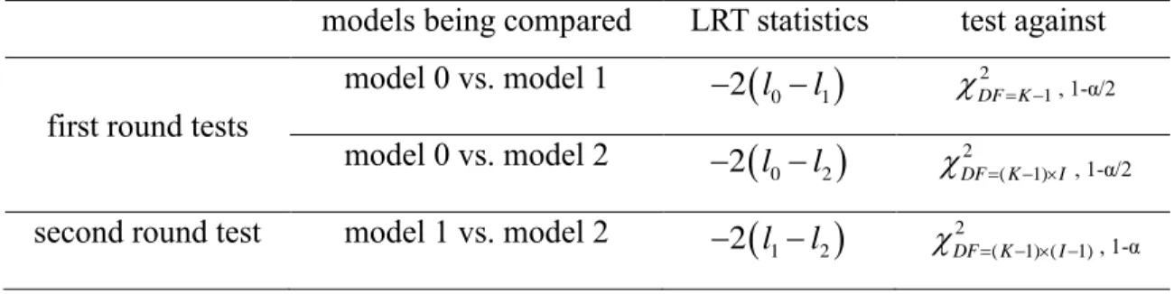
Given a pre-specified significance level α (e.g., 0.05), we perform model selection using the following hierarchical likelihood ratio test (hLRT) procedure (Table 2.2). The first round tests include two parallel tests which compare model 0 vs. model 1 and model 0 vs. model 2, each at significance level α/2. If neither of the two tests is significant, then model 0 is selected. If only one of the two tests is significant, model 1 or model 2 is selected accordingly. If both tests are significant, we perform the second round test which compares model 1 vs. model 2 at significance
14
level α and selects model 2 if this test is significant or model 1 otherwise.
Table 2.2 Summary of hLRT for model selection
models being compared LRT statistics test against
first round tests
model 0 vs. model 1 , 1-α/2
model 0 vs. model 2 , 1-α/2
second round test model 1 vs. model 2 , 1-α
2.2.4 Ranking of differentially spliced genes
When comparing between two biological conditions (e.g., normal vs. diseased), it is often useful to generate a ranking of genes being differentially spliced (i.e., model 2 genes). We rank model 2 genes as follows: Suppose
ˆ
1 and
ˆ
2 are the estimated isoform abundance vectors for the two conditions, we calculate the statistic:1 2 1 1 1 2 1 ˆ ˆ ˆ || ˆ 1 | 2
|
|
|| || ||
|
T ,where ||·||1 denotes the vector L1 norm ([58] uses a similar statistic without the constant 1/2, which
is introduced here to have 0 T 1). Large T values indicate high level of differential splicing.
The T value is 0 for model 0 and model 1 genes. Alternatively, genes classified in model 1 or model 2 can also be ranked according to their p-values from the hLRT, if statistical significance is of major interest.
The proposed approach is implemented as an R package named rSeqDiff, which is available at
http://www-personal.umich.edu/~jianghui/rseqdiff/. The analysis pipeline of using rSeqDiff is provided in Appendix Section A.1.
2.3 Results
0 1
2 l l DF K2 1
0 2
2 l l DF2 (K 1) I
1 2
2 l l DF2 (K 1) (I 1)15 2.3.1 Simulation studies
We study the performance of our proposed hLRT approach by simulating read counts from genes with a wide range of abundances (from lowly expressed genes to highly expressed genes) and report the specificity and sensitivity of our approach for the detection of differential expression and differential splicing events. Detailed procedure and results of the simulation studies are given in Appendix Section A.3, and here we briefly outline the methods that we applied in the simulations. We test differential expression and differential splicing of a hypothetical gene with a well-annotated known isoform structure (Figure A.2) between two biological conditions with sequencing depths of total 50 million and 55 million reads, respectively. The gene structure and the sequencing depths are fixed in the simulations. For each of the three models, we vary the expression level (denoted as G in Appendix Section A.3) of the gene within a broad range, and for each G we simulate the number of reads mapped to each of the two isoforms according to the three models [equations (2.2), (2.3) and (2.4)]. For each G, we simulate 1000 replicated pairs of samples. We run the hLRT with significance level α=0.05 using rSeqDiff on the 1000 simulated pairs of samples and report the proportions of the simulated pairs of samples for which our approach correctly selects the true underlying model (i.e., true classification rate). Table A.1, A.2 and A.3 in Appendix show the true classification rates under model 0, 1 and 2, respectively.
In summary, the simulation studies show that our proposed hLRT approach has well controlled type I error rate at α=0.05 (Table A.1 in Appendix) and good statistical power for detecting differential expression and differential splicing for genes with moderate to high abundance in both conditions (Table A.2 and A.3 in Appendix). When the gene is lowly expressed in one condition but moderately or highly expressed in the other condition, our proposed hLRT approach still has good power in selecting model 1, i.e., differential expression without differential splicing. The power in detecting differential expression or differential splicing is low when the gene has low expression levels in both conditions, which is well expected. In real data analysis, genes with very low expression levels in all the conditions are usually filtered out prior to the analysis. By default, rSeqDiff filters out genes with less than 5 reads in all the conditions.
2.3.2 Applications of rSeqDiff to real RNA-Seq datasets
16
analyzing two real RNA-Seq datasets: the ESRP1 dataset and the ASD dataset.
Analysis of the ESRP1 dataset
Epithelial splicing Regulatory Protein 1 (ESRP1) is a master cell-type specific regulator of alternative splicing that controls a global epithelial-specific splicing network [52]. This dataset was published in [52], where Shen et al performed single-end RNA-Seq experiments on the MDA-MB-231 cell line with ectopic expression of the ESRP1 gene and an empty vector (EV) as control. The dataset contains 136 million reads for the ESRP1 sample and 120 million reads for the EV sample. Shen et al used this dataset to demonstrate their exon-based approach MATS for detect differential splicing, and performed RT-PCR assays to test for 164 exons skipping events. Since the biological significance of this dataset was further analyzed in a follow-up paper by Shen and collaborators [59], our analysis here is solely focused on the validation and comparisons of our proposed hLRT approach with other methods using the 164 RT-PCR tested alternative exons as gold standard.
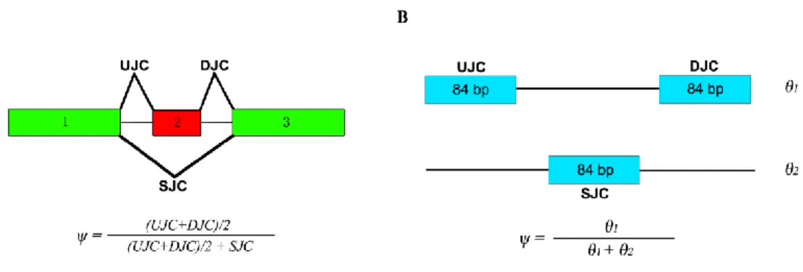
MATS is an exon-based method and its results cannot be directly compared with our isoform-based approach. In the MATS model (Figure 2.2A, modified from [52]), exon 2 is the alternatively spliced exon (skipped exon) unique for the longer isoform and exon 1 and 3 are common exons shared by both of the two isoforms. The exon inclusion level of the skipped exon was defined as the abundance ratio between the longer isoform and the sum of both the two isoforms, which
was estimated as ( ) / 2
( ) / 2
UJC DJC
UJC DJC SJC
by MATS (Figure 2.2A). The exon inclusion level difference between the two conditions (ESRP1 and EV) was calculated as ESRP1EV. The
genome coordinates, junctions read counts (UJC, DJC and SJC), ESRP1 ,EV and
valuesfrom MATS and RT-PCR for the 164 exons are provided in [52]. We first apply rSeqDiff to these 164 exons using only the junction read counts from [52]. We transform the “exon-exon junction model” (Figure 2.2A) to a “two-isoform” model (Figure 2.2B), where the hypothetical “isoform 1” contains two “exons” each with length of 84 bp (the length of the exon-exon junction region in [18]) corresponding to the upstream junction (UJC) and downstream junction (DJC), respectively, and the hypothetical “isoform 2” contains a single “exon” with length of 84 bp corresponding to
17
the skipping junction (SJC). Hence, the abundances of “isoform 1” (1) and “isoform 2” (2) (Figure 2.2B) are equivalent to the abundances of the longer and shorter isoforms in exon-based method (Figure 2.2A), respectively. The exon inclusion level is then estimated as 1
1 2
. For the 164 RT-PCR tested exons, we first use rSeqDiff to estimate 1 and 2 using the junctionread counts (UJC, DJC and SJC) from [52], and then calculate ESRP1,EV and
accordingly.Figure 2.3A shows the scatter plot of the
values estimated by rSeqDiff (using junction reads only) and MATS, and Figure 2.3B shows the scatter plot of the
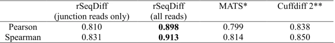
values estimated by rSeqDiff (using junction reads only) and RT-PCR (MATS and RT-PCR results are adapted from [52]). We can see that rSeqDiff gives very similar results as MATS when only junction reads are used, and overall both methods agree well with the RT-PCR assays (Figure 2.3B and Table 2.3).Table 2.3 The correlation coefficients of the
values between RT-PCR and rSeqDiff, MATS and Cuffdiff 2 for the 164 RT-PCR tested exonsrSeqDiff (junction reads only)
rSeqDiff (all reads)
MATS* Cuffdiff 2**
Pearson 0.810 0.898 0.799 0.838
Spearman 0.831 0.913 0.814 0.850
*The values from RT-PCR and MATS are directly adapted from [52].
18
Figure 2.2 Models for estimating the exon inclusion level ψ using the junction reads.
(A) The “exon-exon junction model” used by MATS [18]. Exon 1 and 3 are common exons shared by the two isoforms, and exon 2 is the skipped exon unique for the longer isoform. ψ: exon inclusion level; UJC: number of reads mapped to the upstream junction; DJC: number of reads mapped to the downstream junction; SJC: number of reads mapped to the skipping junction. (B) The “two-isoform model” transformed from (A). The abundances of the longer and shorter isoforms are and , respectively, which are estimated using the junction read counts (UJC,
DJC and SJC).
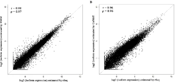
We then apply rSeqDiff using its default settings (detailed method is given Appendix I Section A.4) where all the reads mapped to exons and exon-exon junctions are used [referred as rSeqDiff (all reads) below]. We also run another isoform-based approach Cuffdiff 2 [37,59] on the same dataset (details are given in Appendix Section A.4). These two methods give the estimates of the abundances of all the isoforms. Based on the gene symbols and the genome coordinates of the 164 RT-PCR tested exons in [52], we identify genes containing these exons from the results of rSeqDiff (all reads) and Cuffdiff 2, and calculate the
values for these exons based on the isoform abundances estimated by rSeqDiff (all reads) and Cuffdiff 2. Figure 2.3C shows the scatter plot of the
values estimated by rSeqDiff (all reads) and RT-PCR, and Table 2.3 shows the correlation coefficients of the
values between RT-PCR assays and the three methods, rSeqDiff, MATS and Cuffdiff 2, respectively. We can see that rSeqDiff (all reads) outperforms MATS and Cuffdiff 2 significantly.1
19
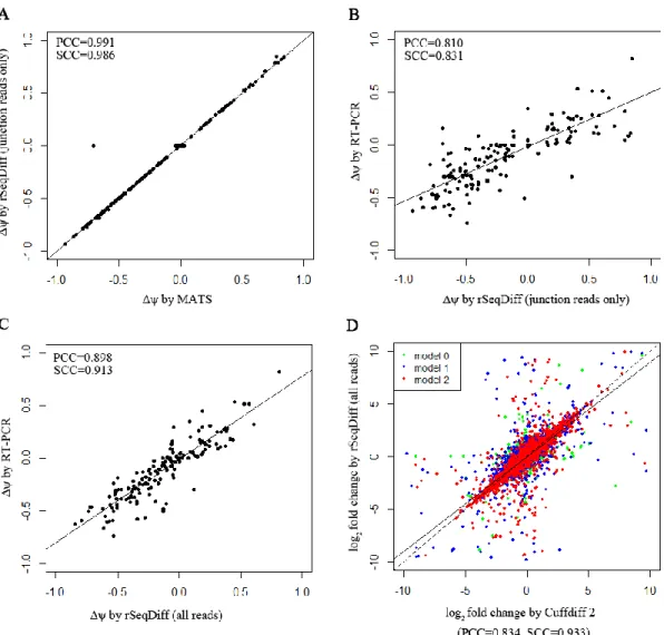
Figure 2.3 Comparisons of rSeqDiff, MATS, Cuffdiff 2 and RT-PCR assays.
(A) Scatter plot of the Δψ values estimated by rSeqDiff (using junction reads only) and MATS. (B) Scatter plot of the Δψ values estimated by rSeqDiff (using junction reads only) and RT-PCR. (C) Scatter plot of the Δψ values estimated by rSeqDiff (using all reads) and RT-PCR. (D) Scatter plot of the log2 fold changes of isoform abundances between ESRP1 and EV estimated by rSeqDiff and Cuffdiff 2. Transcripts classified as model 0, model 1 and model 2 are shown in green, blue and red, respectively. The solid line is the regression line. The dashed line is the y=x line, which represents perfect agreement of the two methods. Δψ: difference of exon inclusion level between ESRP1 and EV; PCC: Pearson Correlation Coefficient; SCC: Spearman Correlation Coefficient.
20
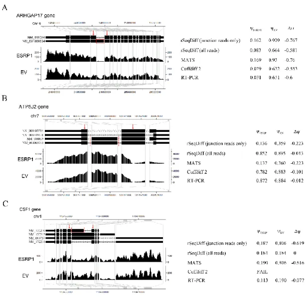
One major advantage of isoform-based approaches like rSeqDiff and Cuffdiff 2 over exon-based approaches like MATS is that isoform-based approaches use all the reads mapped to exons and exon-exon junctions and incorporate the information from all the isoforms rather than using only the local exon structures as shown in Figure 2.2A. The structure of the full length isoforms is important for inferring complex alternative splicing events. Three examples out of the 164 RT-PCR validated exons are given in Figure 2.4. In the first example (Figure 2.4A), the ARHGAP17 gene has only two isoforms differed by an alternative exon. The isoform structure of this gene is relative simple, and all the three algorithms provide similar estimates which are also validated by RT-PCR. In the second example (Figure 2.4B), the ATP5J2 gene has four isoforms differed by an alternative exon in the middle and an alternative 5’ splice site on the exon at the 5’ end. For this gene with a relative complex isoform structure, the two isoform-based methods, Cuffdiff 2 and rSeqDiff, give more accurate estimates than MATS, and rSeqDiff is slightly more accurate according to the RT-PCR result. In the third example (Figure 2.4C), the CSF1 gene has an even more complex isoform structure with four isoforms differed by an alternative exon in the middle and two mutually exclusive exons at the 3’ end. For such an isoform structure, some isoforms (NM_172212 and NM_000757) can only generate upstream junction reads (UJC) for the alternatively spliced middle exon but not downstream junction reads (DJC). As a result, the estimate of MATS is less accurate than that of rSeqDiff. rSeqDiff classifies this gene as model 1, which is consistent with the RT-PCR result. Cuffdiff 2 fails to test (it reports as “FAIL” [59]) this gene due to “an ill-conditioned covariance matrix or other numerical exception prevents testing”. We also compare the estimates of all the gene between rSeqDiff (all reads) and Cuffdiff 2. Cuffdiff 2 fails to test (it reports as “LOWDATA”, “HIDATA” or “FAIL” [59]) several hundred genes with relative complex isoform structures. Figure 1.3D shows the scatter plot of the log2 fold changes of transcript abundances between ESRP1 and EV estimated by the two approaches (genes with low read counts or failed to be tested by Cuffdiff 2 are excluded). Overall the two approaches agree well with each other (Pearson Correlation Coefficient = 0.834, Spearman Correlation Coefficient = 0.933), and the degree of agreement is generally higher when the alternative spliced transcripts are more differentially expressed: the Pearson Correlation Coefficient (PCC) and Spearman Correlation Coefficient (SCC) of transcripts classified in each of the three models are PCC=0.685, SCC=0.802 (model 0), PCC =0.827, SCC=0.932 (model 1) and PCC=0.862,
21 SCC=0.954 (model 2).
Figure 2.4 Examples comparing the estimates between rSeqDiff, MATS, Cuffdiff 2 and RT-PCR assays.
(A) ARHGAP17 gene. (B) ATP5J2 gene. (C) CSF1 gene. The figures on the left show the gene structure and the coverage of reads mapped to the gene visualized in CisGenome Browser [45], where the horizontal tracks in the picture are (from top to bottom): genome coordinates, gene structures where introns are shrunken for better visualization and the coverage of reads mapped to the genes in ESRP1 and EV samples. The table to the right each figure shows the estimates from each method. ESRP1 and EV : exon inclusion levels in ESRP1 and EV, respectively; Δψ: difference of exon inclusion levels between ESRP1 and EV (ESRP1EV).
22
Analysis of the ASD dataset
Increasing evidence has indicated that alternative splicing plays an important role in brain development [60,61] and the pathology of many neurological disorders [62,63]. This dataset was published by Voineagu et al [57], where single-end RNA-Seq experiments were performed on three brain samples of Autism Spectrum Disorder (ASD) patients with down-regulated A2BP1 gene levels (a.k.a. FOX1, an important neuronal specific splicing factor that regulates alternative splicing in the brain) and three control brain samples with normal A2BP1 levels.
In [57], the authors separately pooled the reads for ASD and control to generate sufficient read coverage for the quantitative analysis of alternative splicing events (referred as “pooled dataset” below), and then used an exon-based method similar to MATS in their analysis and detected 212 significantly differentially spliced exons (belonging to 196 unique genes). As we have shown in the analysis of the ESRP1 dataset, the exon-based methods provide less accurate results for complex alternative splicing events and cannot infer the abundances of the isoforms, here we analyze this pooled dataset using rSeqDiff (detailed method is given in Appendix A Section A.5). rSeqDiff classifies 4,507 genes (with 6,850 transcripts) as model 0, 12,374 genes (with 19,556 transcripts) as model 1, 1,769 genes (with 5,848 transcripts) as model 2, and 7,349 genes (with 8,884 transcripts) are filtered out because they have less than 5 mapped reads in both conditions. We also run Cuffdiff 2 [37,59] on this dataset with its default settings. We find Cuffdiff 2 to be relatively conservative for detecting differential expression of spliced transcripts and it only identifies 43 transcripts as significant under default settings (FDR<0.05). Figure A.4 in Appendix shows the scatter plot of the log2 fold changes of transcript abundances between ASD and control estimated by the two approaches (genes with low read counts or failed to be tested by Cuffdiff 2 are excluded). Similar to the analysis of the ESRP1 dataset, the two methods generate concordant results overall (PCC = 0.825, SCC = 0.937). The correlation coefficients for transcripts classified in each of the three models are PCC=0.539, SCC=0.796 (model 0), PCC =0.847, SCC=0.940 (model 1) and PCC=0.854, SCC= 0.953 (model 2), which also show the same pattern as we observed in the ESRP1 dataset. We also run rSeqDiff on each individual biological replicate and get consistent results as the analysis on the pooled dataset (Table A.4 in Appendix).
23
using semi-quantitative RT-PCR assays, and validated 6 of them. Table 2.4 shows the ranking of these genes by rSeqDiff and Cuffdiff 2 (The CDC42BPA gene was not validated in [57]). rSeqDiff is able to detect all the 6 confirmed genes as differentially spliced (model 2) and also gives a more meaningful ranking of these genes than Cuffdiff 2, which might be helpful for biologists to design follow-up experiments. We also compare the estimates of the exon inclusion levels of the six RT-PCR validated exons by rSeqDiff with the exon-based method in [57]. Five out of the six genes (except AGFG1) have concordant annotations for the skipped exons in the RefSeq annotation database are used in our analysis. Table A.5 in Appendix shows the comparisons between the two methods. Basically, rSeqDiff consistently recovers the results from the exon-based method in [57].
Table 2.4 Ranking of RT-PCR validated genes with relevant neurological functions
Genes rSeqDiff Cuffdiff 2
AGFG1 178 5841 RPN2 166 3884 EHBP1 281 8301 CDC42BPA* Model 1 20470 GRIN1 338 6803 SORBS1 208 6313 NRCAM 325 FAIL**
*The RT-PCR result for this gene is not consistent with the exon-based method in [57], therefore this gene is not validated by RT-PCR. rSeqDiff classifies it in model 1.
** FAIL: the gene has an ill-conditioned covariance matrix or other numerical exception which prevents Cuffdiff 2 from testing it [23].
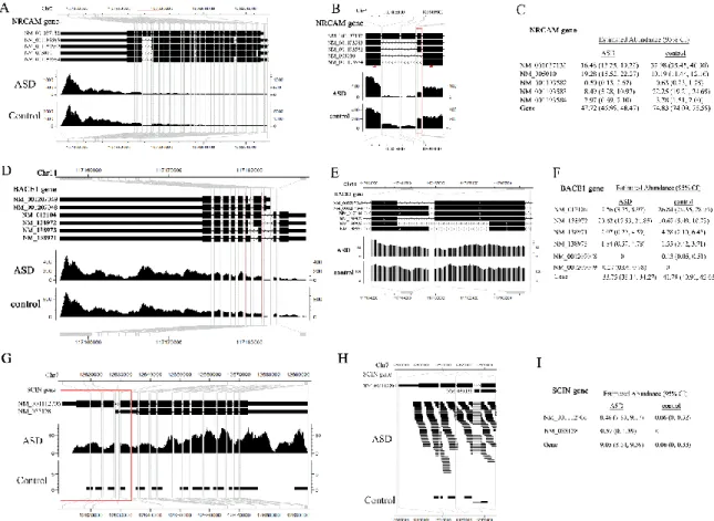
Figure 2.5 shows three examples of genes with differential expression or differential splicing reported by rSeqDiff for the purpose of demonstrating rSeqDiff’s capability in dealing with very complex isoform structures. In the first example (Figure 2.5A-C), the NRCAM gene has five annotated alternative spliced isoforms (Figure 2.5A) and the estimation of their abundances between ASD and control is shown in Figure 2.5C. Figure 2.5B shows the differentially spliced exon that was validated by RT-PCR in [57]. This gene encodes a neuronal cell adhesion molecule
24
which involves in neuron-neuron adhesion and promotes directional signaling during axonal cone growth [64] and has been reported to be associated with ASD by two genetic association studies [65,66]. The second example is the BACE1 gene (Figure 2.5D-F) with six annotated alternative isoforms. This gene has a complex isoform structure, with an alternative 5’ splice site and an alternative 3’ splice site (the part in the red box of Figure 2.5D, enlarged in Figure 2.5E). The estimates of the abundances of the gene and its isoforms are shown in Figure 2.5F. This gene encodes the β-site APP cleaving enzyme 1 (BACE1), which plays an important role in the pathology of Alzheimer's disease [67]. Previous studies show that the isoforms of this gene have different enzymatic activities in the brain [68-70]. Although this gene has not been reported to be associated with ASD, several recent studies have showed that the expression levels of three BACE1 processed protein products, secreted amyloid precursor protein-α form (sAPP-α), secreted amyloid precursor protein-β form (sAPP-β) and amyloid-β peptide (Aβ), have substantial changes in severely autistic patients [71-74]. The third example is the SCIN gene (Figure 2.5G-I) with two alternative isoforms which differ by the mutually exclusive exons at the 5’ end (the part in the red box of Figure 2.5G, enlarged in Figure 2.5H). This gene is identified as model 1 by rSeqDiff, which has a significant higher expression level in autism than control. Also, there is no read mapped to the short exon unique to NM_033128 at its 5’ end (Figure 2.5H), therefore this isoform is estimated to have low abundances in both conditions. This gene encodes Scinderin (also known as Adseverin), a calcium-dependent actin filament severing protein that controls brain cortical actin network [75].
25
Figure 2.5 Examples demonstrating the estimates from rSeqDiff.
(A)-(C) show NRCAM gene. (D)-(F) show BACE1 gene. (G)-(I) show SCIN gene. (A)(D)(G) show the gene structure and coverage of reads mapped to the gene. (B)(E)(H) show enlargement of the parts in the red boxes in (A)(D)(G), respectively, emphasizing the alternative spliced exons. In (B), the red box emphasizes the alternative exon that was validated by RT-PCR assay in [57], and the two red arrows represent the positions of the primers of RT-PCR (see Supplemental Figure 8 of [57]). (C)(F)(I) show estimated abundances for each gene and its isoforms by rSeqDiff. Values in the brackets are the 95% confidence intervals for the estimates.
2.4 Discussion
The two types of approaches for detecting differential transcription across multiple conditions, exon-based approaches and isoform-based approaches, each have their own strengths and weaknesses. Exon-based approaches do not rely on annotated full-length transcripts and provide relatively accurate inference for the differential splicing of a local exon from a gene with relative simple isoform structure [51,52]. However, they cannot provide estimates of isoform abundances and provide less accurate inference for the differential splicing of genes with complex isoform
26
structures. Isoform-based approaches can directly infer isoform abundances and are more accurate for estimating the differential splicing of multi-isoforms with complex splicing events. Since the final functional units are the protein isoforms translated from the alternatively spliced transcripts, isoform-based methods are more biologically informative for follow-up studies. However, isoform-based approaches may give inaccurate estimates if the annotation of full length transcripts is incorrect. We believe that isoform-based approaches will be increasingly used with the improvement of the transcript annotation databases.
One limitation of our approach is that it ignores the biological variations across biological replicates, which will be handled in our future work by extending our model. One way to handle biological variations is to use the negative binomial model as implemented in edgeR [23], DEseq [22], DSS [76] and Cuffdiff 2 [37], where an over-dispersion parameter is introduced and estimated using the empirical Bayes method that borrow information from all the genes. Another way is to use hierarchical Bayesian models, where choosing appropriate prior distributions and efficient parameter estimation (typically using Markov chain Monte Carlo (MCMC) algorithms) are challenging. It is also possible to extend our model to more complicated experimental designs such as crossed experiments by incorporating the covariates into the sampling rate matrix for each sample, since the hLRT is generally applicable to comparisons of complex models.
27
CHAPTER III
rSeqNP: A Non-parametric Approach for Detecting Gene Differential Expression and Splicing from RNA-Seq Data
In this chapter, we present an algorithm, rSeqNP, which implements a non-parametric approach to test for differential expression and splicing from RNA-Seq data. rSeqNP uses permutation tests to access statistical significance and can be applied to a variety of experimental designs. By combining information across isoforms, rSeqNP is able to detect more differentially expressed or spliced genes from RNA-Seq data. The package is available at http://www-personal.umich.edu/~jianghui/rseqnp/. The content of this chapter has been published previously in the journal Bioinformatics [30].
3.1 Introduction
High-throughput sequencing of transcriptomes (RNA-Seq) is a widely used approach to study gene expression [10]. Many statistical approaches have been developed to characterize gene expression variation across RNA-Seq experiments, and many of them are designed for testing differential expression (DE) of genes without considering their alternative spliced isoforms. For a comprehensive review, see [18]. Several recent studies have shown that directly applying the DE approach for detecting differential splicing (DS) may lead to erroneous results, because those approaches do not incorporate the complexity induced by isoform expression estimation for genes with multiple isoforms [37,40]. To this end, several approaches were recently developed to detect differential expression at isoform level [37,39,40,54]. However, there are two remaining issues: 1) many existing approaches only compare between two biological conditions (such as normal v.s. diseased) and their usages for complex experimental designs are thus limited, and 2) most existing