Variable selection optimization for
multivariate classification of metabolomics
data
By
Leslie Romelia Euceda Wood
Thesis for the degree of European Master in Quality in Analytical
Laboratories
Supervisors: Prof. Dr. Bjørn Grung (University of Bergen, Norway)
Prof. Dr. Yizeng Liang (Central South University, PR China)
Research Center of Modernization of Traditional Herbal Medicines,
Central South University, Changsha, PR China Department of Chemistry,
University of Bergen, Norway
Variable selection optimization for
multivariate classification of metabolomics
data
By
Leslie Romelia Euceda Wood
Thesis for the degree of European Master in Quality in Analytical
Laboratories
Supervisors: Prof. Dr. Bjørn Grung (University of Bergen, Norway)
Prof. Dr. Yizeng Liang (Central South University, PR China)
Department of Chemistry,
University of Bergen, Norway
Research Center of Modernization of Traditional Herbal Medicines,
Central South University, Changsha, PR China
CONTENTS
Acknowledgments………... i
List of Abbreviations………...……… iii
Abstract……… vi
1. Introduction………... 1
1.1.Objectives……… 1
1.2.Theory and Background……….. 2
1.2.1. Univariate versus multivariate calibration………. 2
1.2.2. Regression versus classification………. 3
1.2.3. Partial least squares regression……….. 4
1.2.4. Cross validation……….. 7
1.2.5. Classification model assessment……… 8
1.2.5.1.Misclassification error……… 9
1.2.5.2.Accuracy……… 9
1.2.5.3.Sensitivity………... 9
1.2.5.4.Specificity………. 10
1.2.5.5.Area under curve……… 10
1.2.5.6.Mathew’s correlation coefficient………... 11
1.2.6. Variable selection………... 11
1.2.6.1.Competitive adaptive reweighted sampling (CARS)…………. 13
1.2.6.1.1. Monte Carlo sampling………... 13
1.2.6.1.2. Two-stage variable selection using EDF………… 14
1.2.6.1.3. Adaptive reweighted sampling………... 15
1.2.6.1.4. CV to evaluate the variable subset………. 16
1.2.6.2. Subwindow permutation analysis (SPA)……….. 17
1.2.6.2.1. MCS of objects and variables………. 17
1.2.6.2.2. PLS submodel building……….. 18
1.2.6.2.3. Statistical analysis of an output of interest………. 18
1.2.6.3. Random Forest (RF)……….. 20
1.2.6.3.1. Training algorithm……….. 22
1.2.6.3.2. RF for variable selection………. 23
1.2.6.4. Comparison of CARS, SPA and RF………. 25
1.2.7. Instrumentation……….. 26
1.2.7.1. Chromatography……… 26
1.2.7.2. Mass spectrometry……… 30
2. Experimental……….. 32
2.1. Metabolomics datasets……… 32
2.1.1. Type 2 diabetes mellitus dataset (T2DM)……….. 32
2.1.2. Postoperative cognitive dysfunction dataset (POCD)……… 33
2.1.3. Child obesity dataset (CHOB)………... 34
2.2.Data analysis……… 35
2.2.1. Comparison of VS methods………... 35
2.2.1.1. CARS……… 35
2.2.1.3. RF……….. 36
2.2.1.4. PLS-DA model building………. 37
2.2.2. Optimization of VS method………... 38
2.2.2.1. Outlier detection……… 38
2.2.2.2. Analysis of CARS algorithm……… 39
2.2.2.3. Modification of CARS algorithm………. 40
2.2.2.3.1. Top loop: K-fold CV……….. 40
2.2.2.3.2. Outer loop: PLS components for SR calculation… 40 2.2.2.3.3. Middle loop: EDF-ARS runs for VS……….. 41
2.2.2.3.4. Inner loop: PLS components for CV……….. 41
2.2.2.4.New CARS-based method for variable identity and number optimization (VINO)……….. 42
2.2.2.4.1. Stage 1: Obtainment of LV accuracy matrix…….. 43
2.2.2.4.1.1.Top loop: components for SR calculation optimization……….. 43
2.2.2.4.1.2. Outer loop: K-fold CV………... 43
2.2.2.4.1.3. Middle loop: EDF-ARS runs for VS.. 43
2.2.2.4.1.4. Inner loop: components for PLS model building……… 43
2.2.2.4.2. Stage 2: Obtainment of variable number cube, variable identity cube and latent variable mean accuracy matrix……….……….. 44
2.2.2.4.3. Stage 3: Obtainment of fold variable number matrix, fold variable identity matrix and fold latent variable vector……….. 47
2.2.2.4.4. Stage 4: Optimization of variable identity and number and of PLS components for SR calculation and PLS-DA modeling……….. 49
2.2.2.5. Comparison of original CARS performance with that of modified CARS and the new VINO method………. 50
3. Results and Discussion……….. 52
3.1.Comparison of VS methods………. 52
3.2. Optimization of variable selection method………. 54
3.2.1. Outlier detection………. 54
3.2.2. Analysis of CARS algorithm………. 55
3.2.3. Modification of CARS algorithm……….. 59
3.2.4. New method VINO……… 63
4. Conclusion………. 69
5. Future Work………... 71
ACKNOWLEDGEMENTS
First, I would like to thank my supervisor, Prof. Bjørn Grung, for his guidance without which the completion of this thesis would have not been possible. Meetings with you are always interesting and always result in me learning something new, both work related and not. Working with you made me challenge myself to deliver my best effort doing something I was originally not very familiar with. Thank you for your availability and support and also for your help in practical matters related to living in Bergen.
Thanks are also in order for everyone from Professor Yizeng Liang’s group in the Central South University of China (CSU), in which a part of this project was carried out. Special thanks to Professor Liang, Xuxia Long, Yonghuang Yun, Wei Fan and Naiping Dong, who made sure that my stay in China was as pleasant as possible, always available to help with anything I needed. Sharing your culture with me contributed greatly in making my experience there unforgettable, and I will always be grateful for that.
Thank you to Jianhua Huang and Yun Yonghuang, for their direction in the work done in CSU, as well as the contact kept afterwards, always patient and taking time to give explanations, clear doubts and interpret results.
I would also like to thank everyone that makes Erasmus Mundus possible, in particular those who were in charge of ensuring the edition of EMQAL I belong to kept its course throughout its entire duration. Special thanks to those involved from our host institution, the University of Algarve, especially Professors Isabel Cavaco and José Paulo Pinheiro, Telma Costa and the fantastic team from the International Relations and Mobility Office for their patience and for doing their best to provide us an adequate learning environment while making us feel at home.
I would also like to express my gratitude to my EMQAL colleagues and friends. I consider that we all contributed to each one’s successful completion of this program in one way or another. Special thanks to Débora Mendes and Marko Birkic, without whom China
would have never been the same, and to Han Zhu, for guiding us through everything she had already been through in Bergen.
Finally, I would like to thank my family: Gustavo, Miriam, Ana Romelia, Glenda and Allan, for their constant love and support throughout my entire academic process and life in general.
Leslie Romelia Euceda Wood Bergen, May, 2013
LIST OF ABRREVIATIONS
ADA American Diabetes Association
ARS Adaptive reweighted sampling
AUC Area under curve
BMI Body mass index
BSTFA N,O-bis(trimethylsilyl)trifluoroacetamide CARS Competitive adaptive reweighted sampling CART Classification and regression trees
CHOB Child obesity dataset
COSS Conditional synergetic score
CV Cross validation
EDF Exponentially decreasing function
EPA Environmental Protection Agency (USA)
Er Error
FFA Free fatty acid
FLVM Fold latent variable matrix FLVV Fold latent variable vector
FN False negative
FP False positive
FVIM Fold variable identity matrix FVIV Fold variable identity vector FVNM Fold variable number matrix FVNV Fold variable number vector
GC Gas chromatography
IUPAC International Union of Pure and Applied Chemistry LDA Linear discriminant analysis
LV Latent variable
LVAM Latent variable accuracy matrix LVMAM Latent variable mean accuracy matrix LVMAV Latent variable mean accuracy vector
MCC Mathew’s correlation coefficient
MCS Monte Carlo sampling
MPA Model population analysis
MS Mass spectrometry
m/z Mass-to-charge ratio
NIH National Institutes of Health (USA) NIPALS Nonlinear iterative partial least squares NIR Near infrared spectroscopy
NPE Normal prediction error
OOB Out-of-bag
PLS Partial least squares
PLS-DA Partial least squares discriminant analysis POCD Postoperative cognitive dysfunction dataset
PPE Permuted prediction error
RF Random forest
RMSE Root mean square error
RMSECV Root mean square error of cross validation ROC Receiver Operating Characteristic
TMSC Trimethylsilyl chloride
TN True negative
TP True positive
TS Training set
T2DM Type 2 diabetes mellitus dataset
SPA Subwindow permutation analysis
SR Selectivity ratio
UV Ultraviolet
VAM Variable accuracy matrix
VIC Variable identity cube
VIM Variable identity matrix VIV Variable identity vector
VNM Variable number matrix
VNV Variable number vector
VS Variable selection
ABSTRACT
Variable selection is an important step in multivariate calibration in which the number of variables in the independent variable matrix is reduced by eliminating those that are not related to the response. Many methods based on different criteria have been developed for this purpose. Some of them include competitive adaptive reweighted sampling (CARS), subwindow permutation analysis (SPA) and random forest (RF) which can be implemented prior to the construction of both regression and classification models. When applied to metabolomics datasets, variable selection can aid in the discovery of potential biomarkers for a particular disorder.
In this study, the mechanism of the three abovementioned methods described in the literature has been investigated and compared. Their performance when applied to three different metabolomics datasets for multivariate classification was also studied. Although the most favorable method varied for each dataset, model prediction performance was found to improve when variable selection was carried by means of any of the methods. However, because the parameter settings for the methods were set by default for this comparison, an optimization of these is recommended to obtain a more appropriate comparison.
In an attempt to optimize the variable selection stage for the creation of classification models for the three metabolomics datasets of interest, the original CARS algorithm was modified to simultaneously optimize three different parameters. Although promising results were obtained with this modification, a discrepancy was detected in terms of the validation process embedded in the algorithm.
A new variable selection method based on the separate optimization of identity and number of informative variables was developed. However, its implementation did not prove to increase model prediction performance when compared to the results obtained when using the original or modified CARS, or when using all variables in the original dataset. Some of the aspects identified as possible pathways to improve the method’s
performance were tested, only to be discarded. Further study regarding other untested pathways is needed for the improvement of this method.
1.
INTRODUCTION
1.1. OBJECTIVESThe aim of this study was to optimize the variable selection stage prior to the construction of multivariate classification models for three different metabolomics datasets by means of partial least squares discriminant analysis (PLS-DA). To achieve this, the following objectives were defined:
1.1.1. To compare the mechanism of the competitive adaptive reweighted sampling (CARS), subwindow permutation analysis (SPA) and random forest (RF) methods for variable selection as described in the literature.
1.1.2. To perform VS using the three above mentioned methods with standard settings applied to three different metabolomics datasets profiled by gas chromatography (GC)-mass spectrometry (MS).
1.1.3. To examine existing MATLAB scripts for the above methods in detail to verify their mechanism and their accordance to the procedures described in the literature.
1.1.4. To select one of the above methods to modify for improvement by identifying from its algorithm parameters to be optimized.
1.1.5. To establish a strategy and algorithm to simultaneously optimize the identified parameters.
1.1.6. To create a manageable script in MATLAB for the performance of the modified method that allows the user to easily vary the definition of certain input parameters.
1.1.7. To compare the performance of the modified method and the original method applied to the above mentioned three datasets.
1.2. THEORY AND BACKGROUND
Calibration is a widely applied tool in analytical chemistry, without which routine activities as essential as determining the concentration of an analyte in a sample could not be carried out. It is basically a comparison between two sets of numbers, and can be divided into two main types: absolute and relative calibration [1]. Absolute calibration refers to the comparison of a measurement to an accepted standard, for example, the measurement a balance indicates when weighing a standardized mass that is traceable to the international prototype of the kilogram[2]. However, usually in practical quantitative analysis absolute calibration is not really relevant. For example, when using a standard solution of known concentration to calibrate an ultraviolet (UV) visible spectrometer, the purpose is not to obtain a commonly accepted absorbance at a certain wavelength, but to be able to predict the concentration of future samples. This is known as relative calibration, and is how calibration is usually generalized. Martens and Næs define calibration as “the use of empirical data and prior knowledge for determining how to predict unknown quantitative information Y from available measurements X, via some mathematical transfer function”[1].
1.2.1. Univariate versus multivariate calibration
Every calibration model consists of one or more dependent variables, or responses (y), one or more independent variables (x) and their coefficients (β), and an error term (ϵ) which indicates the unexplained variance in the dependent variable[3]. The simplest type of model is the univariate model, in which there is only one independent variable.
Equation 1.
Equation 1 represents the linear relationship between the ith response (y) and its corresponding dependent variable (x). The parameter β0 is the intercept, or the value of y when x is zero[3, 4]; β1 is the slope and represents the change in y for every increase of 1
in x,[3, 4] and ϵ is the error term. The values of β0 and β1 provide the best fitting line for a given calibration data set[3].
Although univariate models can be used to solve some analytical problems, they cannot be applied when there is more than one factor or independent variable affecting the response or dependent variable. Multivariate calibration can be applied to solve complex sample analysis problems where univariate analysis comes short. A typical multivariate model can be represented as shown in Equation 2.
Equation 2.
The parameters β0-βp can be estimated using multiple regression analysis [3, 5, 6]. Multivariate regression is equivalent to univariate analysis in the sense that, when having p number of variables, the values of the parameters or regression coefficients β0, β1, β2… βp return the best hyperplane from relating the dependent variable (y) and the set of independent variables (X)[3].
1.2.2. Regression versus classification
One of the multivariate statistical techniques that study relationships between numerical variables is regression analysis. Regression was first used as a statistical term by Sir Francis Galton in 1877[7], who carried out a study about the height of children born from tall parents. During this study, he named the process of predicting one variable from another “regression”, because he observed that the children’s height tended to move back or “regress” toward the mean height of the population. The term is defined by Gosling as “a statistical technique used to develop a mathematical equation that relates the known variable(s) to the unknown variable”[7]. So, regression analysis is a tool that aids in the estimation of the relationship between the independent and dependent variable(s) through an equation. When there is more than one independent variable involved in the prediction
of the dependent one, as in multivariate calibration, the process is termed multiple regression.
Classification or discriminant analysis is a statistical technique that establishes differences between classes of objects by examining sets of multiple variables corresponding to each object[8, 9]. By identifying these differences, the technique allows the assignment of any object to the class it most closely resembles[9].
Because regression aims to predict a response, while in classification, the purpose is to identify the class which a certain object belongs to, the main difference between the two is the type of values that are obtained for the response variable y: continuous for the former and class labels for the latter[10, 11].
1.2.3. Partial least squares regression
Partial least squares (PLS) is a linear regression technique that is probably the most commonly used method for multivariate calibration [12]. The linear model that results from PLS (Equation 3) consists of a response variable matrix (Y), a descriptive or predictor variable matrix (X), a regression coefficient matrix (β) and a noise or error term (Є) of sizes n by m, n by p, p by m and n by m, respectively. For the matrix X, the number of rows (n) is the number of objects and the number of columns (p) is the number of variables[13]. The columns in the response matrix Y represent the number of responses (m) corresponding to the n objects.
Equation 3.
To establish a PLS model, a weight matrix W of size p by c, where c is the number of latent variables (LV), is calculated for X. LVs are orthogonal or non-correlated factors that provide the best predictions and are derived from the original predictive variables[14]. The factor score matrix T (Equation 4) of size n by c is then calculated. The columns of W
are weight vectors for each of the p columns in X, which are computed in such a way that the covariance between responses and the corresponding scores is maximized [13]. The regression of Y on T is then performed to produce Q, the loadings for Y (Equation 5). Finally, the regression coefficients β are calculated using Q (Equation 6), completing the prediction model (Equation 3).
Equation 4. Equation 5. Equation 6.
The loadings for X (P) of size p by c must also be calculated to obtain the unexplained fragment (F) of the scores (T) in Equation 7.
Equation 7.
Of the available algorithms that can be used to compute PLS, nonlinear iterative partial least squares (NIPALS) is the standard. From the many variants, the following, detailed by Hill and Lewicki [13], who consider it to be one of the most efficient, assumes that both X and Y have been transformed to have means of zero. The superscript T for a given matrix X (XT) represents the transpose [15] of X. For a given vector y, its norm or length [16] is denoted with the symbol || y ||.
For each LV (h), where the initial values for A, M and C are , , , and c is given,
ii. ⁄‖ ‖, and store into as a column
iii. ⁄ , and store into as a column
iv. ⁄ , and store into as a column
v. and vi.
The unexplained fragment F of the scores (Equation 7) obtained with the current LV is used as the next X to estimate the following LV through steps v and vi of the algorithm. At the end of the iteration or repetition for the last LV, the scores matrix T and the regression coefficients β of Y on X can be calculated according to Equation 4 and Equation 6, respectively [10].
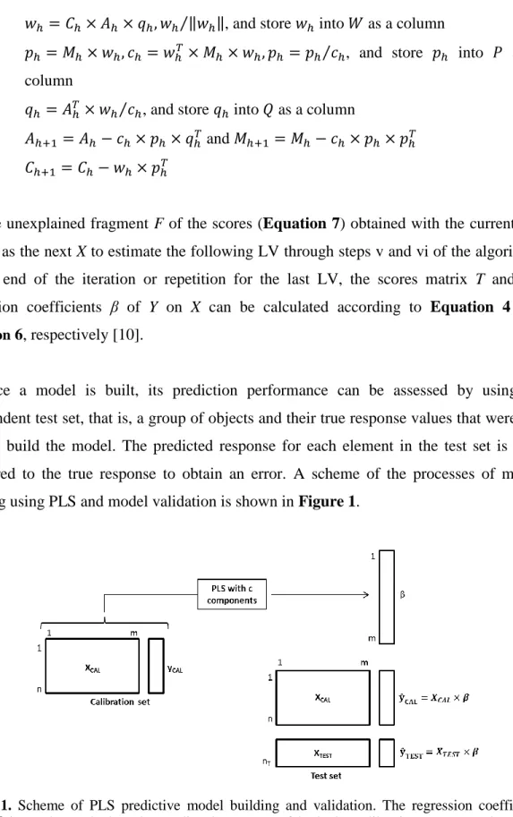
Once a model is built, its prediction performance can be assessed by using an independent test set, that is, a group of objects and their true response values that were not used to build the model. The predicted response for each element in the test set is then compared to the true response to obtain an error. A scheme of the processes of model building using PLS and model validation is shown in Figure 1.
Figure 1. Scheme of PLS predictive model building and validation. The regression coefficient vector β is used to calculate the predicted response of both the calibration set, to evaluate the fitness of the model, and an independent test set, to evaluate the predictive power. (Taken from [12])
PLS-DA is a variant of PLS used for classification problems, when the response y is categorical[17]. It carries out linear discriminant analysis (LDA) on the score matrix T after it has been extracted from the X matrix by PLS. LDA can be implemented through Fisher’s algorithm, which maximizes the variability between classes in relation to the one within the classes[18].
1.2.4. Cross validation
Defining the best number of LVs, or PLS components, for model building is imperative to avoid underfitting and overfitting. A commonly used technique to accomplish this is cross validation (CV) [12]. It consists of partitioning the dataset into a calibration or training set, from which a model will be built, and a validation or test set, which will be used to assess the model’s performance. The partitioning is carried out many times to obtain many different training and test sets, and finally the validation results from all the partitions are averaged.
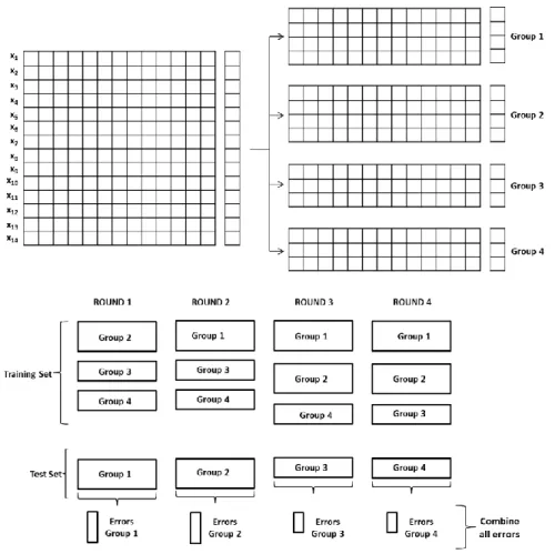
K-fold cross validation is a type of CV in which the data is divided into K non overlapping groups, or folds, of almost the same size[19]. One of the folds is removed and the rest is used to build a PLS model. The fold, which was removed, is then fitted to the model and the response variable predicted by the model is compared to its true response variable to obtain an error. This procedure is repeated as many times as there are groups, until all of them have been used as a test set only once. The prediction errors for all objects are then combined to obtain an error. This error can be calculated for each number of LVs used to build the final PLS model. The number of LVs used to build the model that achieves the lowest error is the optimal one. A new model is calculated from the entire dataset using the optimal number of components revealed at the end of the CV procedure. An example of 4-fold CV is represented in Figure 2.
Figure 2. Representation of a 4-fold CV example using a predictive variable matrix X of size 14 by 13 and only one response y for each of the 14 objects. The objects are partitioned into four different groups which alternate the role of test set in each different CV round. The errors of each group are combined to obtain one final error.
1.2.5. Classification model assessment
Regression and classification differ mainly in the type of values the response variable contains. Since these are continuous for the former, a root mean square error (RMSE) proves to be appropriate to assess model prediction in this case. However, this parameter cannot be applied for classification models as the values recorded in the response are categorical. Other parameters exist as alternative assessment parameters for classification. The ones used in this study are described below. Because this study involved binary classification problems, the following descriptions can be applied to this particular situation, disregarding cases in which more than two classes are to be predicted.
1.2.5.1. Misclassification error
The misclassification error is the total number of incorrectly classified objects, comprising false negatives (FN) and false positives (FP), divided by the total number of classified objects (n) (Equation 8) [20].
∑( ̌ )
Equation 8.
1.2.5.2. Accuracy
Subtracting the misclassification error from one generates the model prediction accuracy [20, 21]. This parameter is a measure of how well a model can assign the correct class to an object from unknown or test data [22]. Being the opposite of the misclassification error, it can also be calculated by dividing the number of correctly classified objects, consisting of true negatives (TN) and true positives (TP), by the total number of classified objects (n) (Equation 9).
∑( ̌ )
Equation 9.
1.2.5.3. Sensitivity
Sensitivity is a measure of a model’s ability to correctly classify objects with positive value or of class 1 [23, 24]. Let us consider that, for a given dataset in which the objects represent individuals, class 1 and -1 indicate the presence or absence, respectfully, of a particular disease or condition. A highly sensitive model would produce few false negatives, meaning that most of objects of class 1 would correctly be associated with the condition at issue [24]. This parameter is calculated by dividing the number of correctly classified objects of class 1, or TPs, by the total number of objects of class 1 that were classified, or TPs and FNs (Equation 10).
Equation 10.
1.2.5.4. Specificity
Specificity is a measure of a model’s ability to classify objects of negative value or of class -1 [23, 24]. For the example described for sensitivity (Section 1.2.5.3), a highly specific model would be one that produces few false positive results. This means that most of the objects of class -1 would correctly be associated with the absence of disease [24]. This parameter is calculated by dividing the number of correctly classified objects of class -1, or TNs, by the total number of objects of class -1 that were classified, or TNs and FPs (Equation 11).
Equation 11.
1.2.5.5.Area under curve
The area under the receiver operating characteristic (ROC) curve, or simply area under curve (AUC), is a measure of a model’s ability to discriminate objects of different classes [25]. It plots the rates of correctly classified objects of class 1, or TPs (sensitivity), against the rates of incorrectly classified objects of class -1, or FPs (1-specificity) for an entire range of cut points (Figure 3) [25, 26]. AUC values range from 0.5 to 1.0, the latter indicating perfect classification ability (100% sensitivity and specificity) and the former a random choice of class (50% sensitivity and specificity) [27, 28].
Figure 3. A) ROC curve with AUC close to 1, indicating high discriminatory power and B) ROC curve with AUC of 0.5, a diagonal line, indicating no discriminatory power. (Taken from [28])
1.2.5.6. Mathew’s correlation coefficient
Mathew’s correlation coefficient (MCC) is a measure of the correlation between the predicted value and the true response [29]. MCC values range from 1 to -1, indicating perfect positive or negative correlation, respectively. A value of zero indicates orthogonality, or total absence of correlation. MCC is calculated according to Equation 12.
√( ) ( ) ( ) ( ) Equation 12.
1.2.6. Variable selection
Variable selection (VS) is the process of reducing the original number of explanatory variables in the dependent variable X matrix by discriminating informative variables from the ones that are not related to the response y [30]. Some of the reasons why VS is an important step in the calibration process include the following:
a) According to the parsimony principle, also known as Ockham’s razor, for a group of competing models that fit a given dataset, the simplest should be considered the best one[31, 32]. In other words, the data should be explained in the simplest way; thus, unnecessary or uninformative variables that do not have any effect on a prediction should be excluded[33].
b) Some variables are not only uninformative, but they are also interfering. That is, they add more noise than relevant information to the model and their inclusion actually makes an analytical prediction worse[33, 34].
c) Cost in terms of time and money can be reduced if irrelevant predictors are not measured [33].
d) The selecting of informative variables can be applied for different purposes such as identifying the most influential factors affecting the quality of a product or the characteristic features of a certain class. In the first instance, a few vital factors are much easier to measure and control in a process industry than all possible process variables [35]. The second case takes place, for example, when classifying metabolomics data.
In a metabolomics dataset, each variable represents a metabolite, and the objects are individuals. In the case of binary classification, there are only two possible responses: 1, indicating the presence of a particular metabolic state, such as a disorder, or -1, indicating its absence. So by selecting informative variables from these types of datasets, a selection of informative metabolites, that can be considered potential biomarkers, is actually taking place[36, 37, 38]. In this way, we can learn about metabolic perturbations that exist in individuals with a disease of interest, and ultimately, determine the pathophysiological mechanisms of the disease, allowing the discovery of new pathways for diagnosis and treatment.
The purpose of VS is to find a subset of variables that produce the smallest errors when used to carry out quantitative analysis or to classify objects into different categories[34]. Many methods have been developed to either identify variables that provide relevant
information, eliminate interfering and uninformative variables or both. Three of these methods are described below.
1.2.6.1.Competitive adaptive reweighted sampling (CARS)
CARS is a method originally developed to select informative wavelengths from continuous spectral data, specifically applied for the first time to near infrared spectroscopy (NIR) [39]. It is based on Darwin’s evolution principle “survival of the fittest” and is combined with PLS to assess variable importance. It basically consists of a number of iterations involving 1) Monte Carlo sampling (MCS) in object space, 2) VS by means of weights and the exponentially decreasing function (EDF), 3) VS by reweighted sampling of variables selected in the previous step and 4) model building with each subset of selected variables and CV to calculate prediction error.
1.2.6.1.1. Monte Carlo sampling
The first step in the CARS algorithm involves obtaining a sample of objects using the Monte Carlo approach to build a multivariate model. The name “Monte Carlo” was properly attributed after the popular gambling destination, as this sampling method is based on the laws of chance or probability[40]. A sample of objects is selected randomly without replacement, which means that an object that was chosen does not return to the sampling lot and thus, can only be sampled once. The ratio of kept objects for training or model building is usually around 0.80-0.90[39]. The remaining unsampled objects will not be used during that particular iteration until the fourth step where all objects will be included for CV to obtain a prediction error. This sampling is done to “select variables which are of high adaptability regardless of the variation of training samples” [39]. In other words, the aim is that the method is as robust to the change in samples used for model building as possible. Some of the parameters resulting from the PLS model built from the training sample obtained in this step can be used to calculate an importance score for each variable.
1.2.6.1.2. Two-stage variable selection using EDF
A weight (w) is calculated as an importance score based on the regression coefficient (β) corresponding to each variable (Equation 13).
| |
∑ | |
Equation 13.
where p is the number of variables in the original dataset. An alternative importance score to use here is the selectivity ratio (SR), which is the relation between the explained (vexp) and residual (vres) variance for each variable[37, 41] (Equation 14).
⁄ Equation 14.
The explained and residual variance should be calculated based on target projection [41], which “reveals the y-relevant variation in the x-variables captured by a multicomponent PLS model on a single latent variable” [41].
The variables with the highest weights or SRs will be kept. The ratio of variables to be kept for each MCS run will vary, and is calculated based on (Equation 15):
Equation 15.
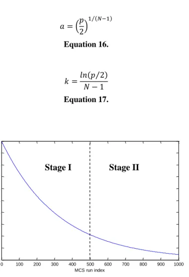
where N is the number of the MCS run or iteration that is taking place and a (Equation 16) and k (Equation 17) are constants that follow two conditions: I) For the first MCS run, all variables will be selected in this step, II) while in the last run, only two variables will be kept. In this way, the ratio of variables to be kept (r) will decrease for each run (i), exhibiting a behavior that can be graphically observed in Figure 4. The decrease is exponential and occurs in two stages: I) rapidly, where the number of chosen variables
drops significantly between iterations and II) subtly, where the number of variables kept varies very little in comparison to the previous iteration[39].
( ) ( )⁄
Equation 16.
( ⁄ )
Equation 17.
Figure 4. Exponential decrease of the ratio of retained variables in Step 2 of the CARS algorithm for each MCS run. Two stages can be distinguished: I) a rapid decrease in the number of retained variables and II) a more refined selection where the number of kept variables varies very little in comparison to the previous sampling run. (Taken from [39])
1.2.6.1.3. Adaptive reweighted sampling
The third step of the CARS algorithm consists of a second variable selection process and is where the evolution principle is applied. Based on their weights or SRs, the higher the importance score, the more fit or competitive a variable is to survive. Variables with lower importance scores are weaker and will be wiped out by the more dominant ones. This process is carried out by the use of adaptive reweighted sampling (ARS), where the higher the importance score assigned to each variable in Step 2, the higher the probability
0 100 200 300 400 500 600 700 800 900 1000 0 0.1 0.2 0.3 0.4 0.5 0.6 0.7 0.8 0.9 1 MCS run index R a ti o o f re ta in e d v a ri a b le s Stage I Stage II
for its corresponding variable to be sampled. In this way, by means of sampling with replacement, in which a variable is selected and then returned or “replaced” to the population which is being sampled[42], the variables with higher scores will be sampled multiple times, while the ones with the lower scores will be completely left out, and thus, eliminated. The variables that were sampled more than once have taken the place of those that were discarded; thus, the resulting vector is the same size as the one containing the variables that were submitted to ARS. Finally, the remaining variables are included only once in the final selected variable subset, regardless of how many times they were resampled, resulting in a variable vector of reduced size.
1.2.6.1.4. CV to evaluate the variable subset
Finally, a PLS model is built considering only the variable subset selected in steps 2 and 3, and an error is obtained using CV. As mentioned before, CV evaluates model prediction by dividing the data into multiple training sets and independent test sets[43]. The objects included in the training and test sets are alternated in such a way that each object is in the test set once and once only[43]. The error obtained will either be a root mean square error of cross validation (RMSECV) or a classification assessment parameter, in the case of regression or classification, respectively.
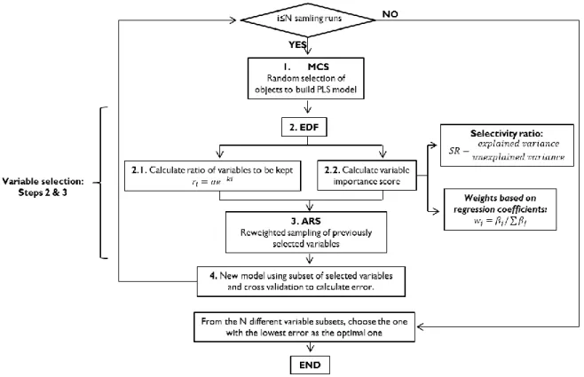
The four steps above will be repeated for each MCS run or iteration, obtaining an error for each one. The run whose error is the lowest will be considered the optimal one, and the variable subset obtained in that run will be selected as the best combination of variables for predictive purposes. Figure 5 summarizes the CARS algorithm in a flow chart.
Figure 5. Flow chart of CARS algorithm.
1.2.6.2. Subwindow permutation analysis (SPA)
SPA was developed to be applied to metabolomics datasets for the selection of metabolites that could be informative of the prediction of a clinical outcome, thus considered biomarkers [36]. It is based on the principles of model population analysis (MPA) and like CARS, uses PLS to build a series of submodels. MPA’s main principle is to statistically analyze an output of interest of a population of sub-models[44]. In the case of VS, one could analyze the distribution of prediction errors[36]. In summary, the steps to execute SPA are: 1) MCS in object and variable space, 2) PLS submodel building for each sampling run and 3) statistical analysis of the distribution of prediction errors.
1.2.6.2.1. MCS of objects and variables
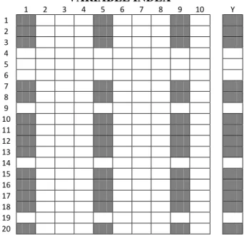
Unlike CARS, MCS is performed on variables as well as objects for each run (Figure 6), resulting in a data subwindow which gives, to some extent, information about the synergetic effect between the variables included in it[36]. This effect refers to the higher
SAM P L E I ND E X
performance of the combination of variables when compared to that of the sum of the individual contributions of each one[36].
VARIABLE INDEX 1 2 3 4 5 6 7 8 9 10 Y 1 2 3 4 5 6 7 8 9 10 11 12 13 14 15 16 17 18 19 20
Figure 6. Representation of MCS in both object and variable space for a dataset of size 20 X 10, if a ratio of 0.75 objects and a number of 3 variables are retained for each subwindow. The resulting training set would be of size 15 X 3, while the test set would comprise the remaining 5 objects and the same 3 variables. (Taken from [36])
1.2.6.2.2. PLS submodel building
When solving classification problems, PLS-DA can be used to build models with the training sets of each subwindow. CV is employed to choose the optimal number of PLS components.
1.2.6.2.3. Statistical analysis of an output of interest
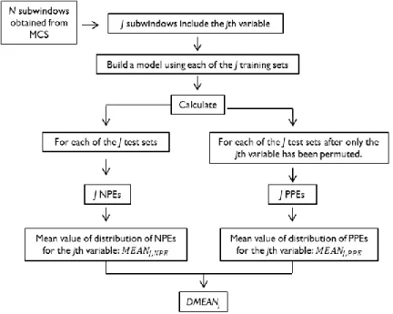
As mentioned before, for the purpose of VS, a suitable output to analyze is the distribution of the prediction error. For N MCS runs, the same number of subwindows will be obtained. However, not all of the N subwindows will contain the jth variable; so, in order to assess its importance, only the J subwindows that contain it should be analyzed.
The J submodels obtained from the previous step will be validated using their corresponding J test sets, for which two errors will be calculated: a normal prediction error (NPE) and a permuted prediction error (PPE). The difference is that the second one is calculated using the test set after randomly permuting, or giving a random order to the values for the jth variable. In this way, the variable of interest is being noised up and so, if it is considered predictive, the prediction error would be expected to increase[45] because the accuracy of the output depends on the specific value of this variable. A DMEAN is obtained by subtracting the mean of NPEs from that of PPEs (Equation 18). The procedure is illustrated in Figure 7.
Equation 18.
Figure 7. Obtainment of NPEs and PPEs for the calculation of variable importance assessment parameter DMEAN.
Each NPE and PPE is dependent of the combination of variables belonging to their corresponding subwindow, hence providing information regarding the interactions between
those variables. The whole J subwindows encompass the effects that all of the p-1 variables have on the variable j[36].
The variable selection process consists in I) eliminating all variables with a DMEAN lower than zero, II) carrying out Mann-Whitney U-Test to evaluate the significance in the difference between the distributions of both prediction errors, resulting in a ρ-value for each variable, III) variable ranking according to their ρ-value and IV) selecting the variables that comply with a predefined threshold.
The Mann-Whitney U-Test can be considered “the non-parametric equivalent of Student’s t-Test” [46] whose use does not require data to be normally distributed. This statistical test checks whether the data of a particular group tends to be larger than that belonging to another group [47].
The ρ-value is inversely proportional to variable importance, and thus, for practical reasons, it can be converted to a conditional synergetic score (COSS) through Equation 19. In this way, the score assigned to each variable is directly proportional to its importance, and therefore the acceptance criteria will change, for example, from ρ≤0.01 to COSS≥2.
( )
Equation 19.
1.2.6.3. Random Forest (RF)
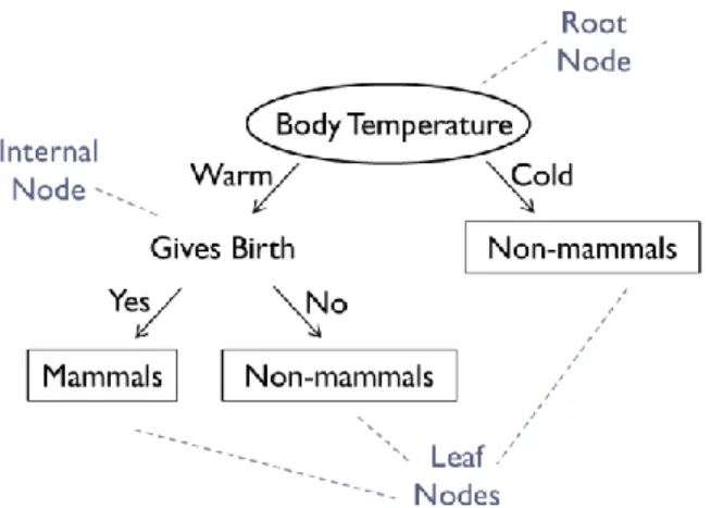
RF is an ensemble method, which combines multiple decision trees to obtain one final prediction[48]. A decision tree is a hierarchical structure consisting of nodes and directed edges which is built by crafting a series of key questions about the attributes of certain data of interest [49]. Three types of nodes make up a decision tree: a root node, which has outgoing edges but no incoming ones; internal nodes, which have both incoming and outgoing edges; and terminal or leaf nodes, which only have incoming edges, and denote a
label or prediction. The root and internal nodes, being non-terminal, contain attribute test conditions to separate objects that have different characteristics[49].
To illustrate this, Tan, Steinbach and Kumar [49] present a decision tree for the classification of mammals or non-mammals (Figure 8). When an object is run down the tree, the answer to the question “body temperature” will lead to either a follow-up question, or a classification label. In this way, as many follow-up questions will succeed until a final conclusion about the object is made.
Figure 8. Decision tree classifier for the mammal classification problem. Three types of nodes can be distinguished, where the leaf nodes designate the final outcome or prediction. (Taken from [49])
Although decision trees have the advantages of being able to handle high-dimensional data, ignore unimportant variables and interpret models suitably, their performance is not always satisfactory. The simple decision tree illustrated above (Figure 8) fails to correctly classify the monotremes, which are a special group of mammals that lay eggs instead of giving birth [50], such as the platypus. In general, decision trees usually have low prediction accuracies[51], only slightly better than a random choice of class[48]. One of the attempts to improve this has been the use of ensemble methods or combining forecasts, which combine the results of multiple individual models to reach a single prediction[52]. Experimental evidence has shown that ensemble methods are often much more accurate than any single hypothesis[48, 53].
For a given data subset used to build a decision tree, the conditions that separate an object in each of the non-terminal nodes according to its known response (y) will be governed by the “attributes” of each object in the training set, these being represented as a p-dimensional vector of variables associated with each object [48]. Thus, RF can be defined mathematically as an ensemble of B trees { ( ) ( )}, where { } is a variable vector corresponding to an object whose outcome will be predicted [51]. A total of B predictions will be obtained for each object: { ̌
( ) ̌ ( )} , one from every tree, all of which will then be combined to produce one final prediction [51]. RF can be used to solve both regression and classification problems, being the final outcome the average of all individual tree predictions for the former or the class obtained by the majority of trees for the latter[51, 52].
1.2.6.3.1. Training algorithm
The following training procedure has been taken from Svetnik et al. [51]. Given data for a set of n objects for training, D = {(X1, Y1), …, (Xn, Yn)}, where Xi, i=1, …, n, is a vector of variables and Yi is the corresponding prediction for the ith object, the algorithm is as follows:
i. From the training data of n objects, a bootstrap sample is drawn, which is a random sample with replacement of size n. This means that the new sample will have the same number of objects as the original one; it could include some of the original objects more than once, while others will be left out altogether[54]. The selection of an object for the new sample is independent from the previous selection.
ii. For each bootstrap sample, a tree is constructed by choosing the best split at each node, among a randomly selected subset of mtryvariables, instead of all of them. Here, mtry is a tuning parameter that can be chosen as a function of the total number of variables (p). The performance of RF seems to change very little over a wide range of values of mtry, except near the extremes: 1 or p. The
tree is grown until no further splits are possible, reaching its maximum size, and it is not pruned back.
iii. The above steps are repeated until a sufficient number of trees are grown.
The tree growing algorithm used is CART (Classification and Regression Trees), that builds classification trees according to a splitting rule; the rule that performs the splitting of the training sample into smaller parts[55].
1.2.6.3.2. RF for variable selection
The construction of each decision tree depends on random vectors sampled independently from each other, but with the same distribution for all trees in the forest [48]. This refers to bootstrap sampling[54], and the random vectors sampled are the p -sized vectors of variables corresponding to each object in the training set. Thus, the selection of an object for training is independent of the previous one. This means that some objects will be sampled more than once, while others will not be sampled at all[54]. The former will constitute the bootstrap sample, which is the same size of the original dataset [54], with the difference that it contains repeated objects, and will be used for trainng or tree construction. The rest of the objects constitute the out-of-bag (OOB) sample, which is the test set, and will be approxmately one third of the size of the original dataset [51]. According to empirical evidence provided by Breiman [48], having this large test set is almost as accurate as it being the same size as the training set.
Variable importance in RF is carried out by means of the OOB estimates. Due to its complexity, the mechanism of how a group of trees provides a prediction is difficult to interpret. Because it does not produce an explicit model, the relationship between descriptors or variables and the outcome is said to be hidden inside a “black box” whose insides are practically unknowable [51, 56, 57]. To solve this problem, internal OOB estimates can be used to carry out certain measures of variable importance that are available to identify the informative variables[56].
As an approach to measure the importance of the jth variable, two measurements of prediction performance are computed for the test set or OOB sample, in a similar way as described in Section 1.2.6.2.3 as NPEs and PPEs for SPA. Each OOB object is run down its respective tree to obtain a prediction. In addition, a second run is carried out, this time permuting the jth variable. At the end of the procedure, each object will have two predictions for each time it constituted the OOB sample for a given tree: a normal prediction and one carried out with the jth variable permuted or noised up.
The performance of each prediction must then be measured. As stated by Svetnik et al. [51], in the case of classification problems, the change in prediction accuracy is usually a less sensitive measure than the change in the margin. For multiclass classification problems, margin can be defined as the difference between the proportion of correct class predictions and the maximum proportion of incorrect ones [58]. Svetnik et al. [51] illustrates this by supposing for a given three-class problem that an object of class 1 receives 60, 30 and 10 percent votes of class 1, 2 and 3 respectively. Thus, the margin is equal to ( ) . In the case of binary classification, the margin is simply the difference between the proportion of correct class predictions and the proportion of incorrect ones. A positive margin indicates a correct class prediction, while a negative one means the opposite[51].
From the margins calculated for normal predictions and predictions with permuted variable j, the means for both, M and Mj, respectively, are calculated. The variable importance is simply the difference between these means (Equation 20), where if it is positive, zero or negative, the variable is considered informative, non-informative or interfering, respectively. For regression problems, the RMSE is calculated instead of margins[51].
Equation 20.
1.2.6.4. Comparison of CARS, SPA and RF
From the literature search carried out, a series of aspects have been identified in which CARS, SPA and RF can be compared.
In general, they are all based on different criteria: CARS on a variable importance score based on parameters obtained from the construction of a PLS model; SPA on the difference in empirical distribution between NPEs and PPEs; and RF on the difference in prediction performance validated on OOB estimates with normal and permuted variable values. Unlike the other methods, which were developed for classification purposes, CARS was originally meant to solve regression problems.
Regarding the selection of objects used for the training procedure, RF uses bootstrap sampling, while the others use MCS. However, during this sampling procedure, both SPA and RF also select a subgroup of variables for training in each run. The original model built in CARS in each run, on the other hand, includes all variables in the dataset.
All of the methods involve a validation stage to generate an error that is used in some way to select the optimal variable subset. SPA and RF calculate a normal error and an error when the values of a certain variable are randomly permuted from an independent test set. CARS carries out CV on the original dataset to obtain an error; thus, because most of the objects are used for training the PLS model in the first step, the test set is not independent.
Finally, the criteria for the selection of variables once the importance scores for each one is known varies between all methods. CARS automatically produces a subset that achieves the lowest error, that was selected by EDF and ARS based on the individual variable importance scores. SPA and RF assign errors to each variable individually, as opposed to doing so to a set of variables as in CARS. However, RF only focuses on the sign of the importance score, designating variables as informative, noninformative or interfering if this is positive, negative or zero, respectively. SPA on the other hand, calculates a ρ-value or COSS for each variable, and defines a threshhold or cutoff value for
one of these, or both, as criteria for variable selection. Table 1 summarizes the similarites and differences between the VS methods at issue.
Table 1. Comparison between the methods of CARS, SPA and RF for VS.
CARS SPA RF General Criteria: Regression coefficients or SRs obtained from PLS Difference in empirical distribution between NPEs
and PPEs
OOB estimates to validate performance
using normal and permuted variable values
Developed for: Regression Classification Classification
Sampling for
training set: MCS MCS Bootstrap sampling
Training set
sampling of: Objects Objects & variables Objects & variables Error(s) generated
from validation stage: CV error NPE & PPE NPE & PPE
Validation performed
on: All data Independent test set
Independent test set (OOB samples)
Criteria for VS: with the lowest error Subset associated
Variables achieving a ρ-value below or a COSS above a defined threshold
Variables with positive importance score
1.2.7. Instrumentation
Of the available analytical techniques used to generate data from chemical systems prior to multivariate analysis, gas chromatogarphy (GC) coupled with mass spectrometry (MS) is applied in many fields because of its versatility to separate, quantify and identify volatile and semi-volatile organic compounds[59, 60]. It combines the advantages of high degree of separation, or resolution, from GC, and strong identification power, or high sensitivity, from MS [61].
1.2.7.1. Chromatography
The International Union of Pure and Applied Chemistry (IUPAC) defines chromatography as “a physical method of separation in which the components to be separated are distributed between two phases, one of which is stationary (stationary phase) while the other (the mobile phase) moves in a definite direction” [62]. The signal obtained
by the chromatographic system is related to the concentration of the separated compounds and is represented graphically in a chromatogram. A chromatogram is a plot of the signal in function of time or of volume of used mobile phase in the form of peaks[63]. It can provide qualitative or quantative information by determining the position of the component’s peaks in the time axis or by calculating the area under the peak, respectively [63].
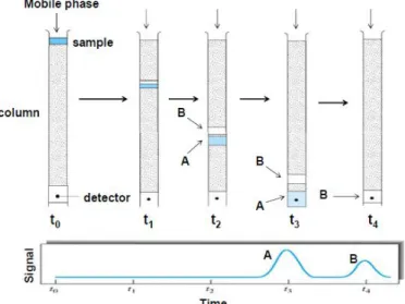
Elution in chromatography is the process in which a sample is dragged by the mobile phase through the stationary phase, which is contained in a chromatographic column. The more affinity a certain compound in the sample has to the composition of the stationary phase, the longer it will be retained in the column, because it will be more difficult for the mobile phase to drag it. If a sample has no affinity to the stationary phase, it will not be retained by it, and will simply move along with the flow of the mobile phase. Thus, the compounds that are less retained by the stationary phase, will flow faster and will exit the column to the detector first. The last compounds detected are the ones that have more affinity to the stationary phase. Figure 9 shows a scheme of the previous description.
Figure 9. Scheme of the chromatographic elution process. The mobile phase flows continuously through the column, which is packed with the stationary phase. Of the compounds in the sample, B
has more affinity to the stationary phase, and so is retained longer. Compound A exits the column and is detected first (t3) and B follows after a certain time (t4), thus being separated. (Taken from [64])
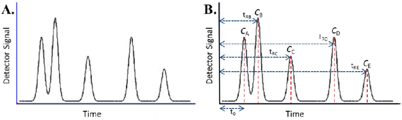
Compound A (CA) in Figure 10 is the unretained species, and so t0 is the dead time, which gives a measure of the mobile phase migration rate [63]. The retention time tR for each compound is actually the sum of the dead time with the time the compound was delayed in exiting the column at regular time with the mobile phase (ts) due to its retention in the stationary phase (Equation 21). Knowing the length of the column (L), the average linear velocities of both the mobile phase (Equation 22) and each solute or compound separated (Equation 23) can be calculated.
Equation 21. Equation 22. Equation 23.
Figure 10. Example of a chromatogram (A) and its basic parameters (B). The retention time tR of
each compound C is the time it takes to travel through the chromatographic column which contains the stationary phase. CA is an unretained species, and so its elution time is the dead time (t0).
The different types of chomatography mainly vary in the physical state of the mobile phase. In GC, it is a gas, and the stationary phase is either a solid, (gas-solid
chromatography) or a liquid (gas-liquid chromatography), making its interaction with compounds an adsorption, or a partition, respectively. In the latter, the compounds are dissolved in the mobile phase, not just attached to its surface like in the former[65]. The sample is vaporized when it is injected in the column and the first compounds to elute tend to be the ones with lowest boiling point or most volatile[66].
The main parameters that affect the resolution or separation ability in GC are the temperature, the flow rate of the mobile phase or carrier gas, the composition of the stationary phase and the column dimensions[67]. The chromatographic system consists in a) a carrier gas supply with pressure and flow rate regulators, b) an injection system c) a column, d) a detector and e) a read out or recorder system (Figure 11).
Figure 11. Scheme of a GC system and its components. (Taken from [66])
The continuos flow of the carrier gas is carefully controlled, resulting in relatively precise retention times. The sample is injected in liquid or gas phase, and once in the injector, it is vaporized and homgenized with the carrier gas and swept by it into the column. The column is usually a tube wound in a spiral of 1 to over 100 m long[63] and is usually inside an oven with a wide range of temperature settings. After the sample has travelled through the entire column, it passes through the detector and then is dispersed in the atmosphere.
1.2.7.2. Mass spectrometry
Although GC offers advantages such as high resolution, speed and relatively low cost, it usually requires the use of spectroscopy to confirm the identities of the peaks[61, 67]. One of the reasons GC and MS are highly compatible is that both need the sample to be in the gas phase[61]. Instead of the dispersion of the sample into the atmosphere after GC analysis, coupling can be carried out by simply connecting the end of the column to the entrance of the MS system wih a transfer line (Figure 12). The vaporization and separation of the components in the sample performed by GC can be considered a “pretreatment” before MS analysis.
Figure 12. Coupling of a gas chromatograph and a mass spectrometer. (Taken from [68])
Fenn et. al. [69] defined MS as “the weighing of individual molecules by tranforming them into ions in vacuo and then measuring the response of their trajectories to electric and magnetic fields or both”. After the sample is introduced in the mass spectrometer, three basic operations take place: 1) ionization, 2) separation of the ions based on their mass-to-charge ratio (m/z) and 3) counting of the number of ions in each seperated group or measuring the ion current during ion formation [63]. The m in m/z refers to the atomic mass of the ion while the z is its elementary charge. Usually the ions formed have a single charge [63]; thus, the m/z in most cases is merely the atomic mass of the ion. The mass spectrometer’s response is represented in a plot of relative intensity in function of m/z (Figure 13).
Although there are many types of mass spectrometers with varying ion sources and mass analyzers, they all consist of the same basic components (Figure 14). The ion source transforms the introduced sample into gaseous ions by bombarding it with electrons, photons, ions, molecules or thermal or electric energy. The ions produced, which are usually positive but can also be negative, are then accelerated into the mass analyzer. Here, the energetically charged ions are continuosly detected and sorted according to their m/z. Finally, the beam of ions is converted into an electric signal by a transducer to be processed and displayed in a further stage. It is important to note that all the components, with the exception of the last, are maintained in a vacuum, or at a pressure lower than the atmosphere’s. The object of this is to reduce the frequency of collisions to ensure the integrity of the ions and electrons produced[63].
Figure 13. Mass spectra of the compound C10H14O shown. (Taken from [70])
Figure 14. Basic components of a mass spectrometer. (Taken from [63])
The resulting mass spectra can be compared with existing spectral libraries until a match is obtained, and thus the compound is identified.
Chromatographic techniques coupled with MS have been recognized as the standard for metabolomic profiling[71, 72]. Of these, the combined advantages of GC-MS mentioned before, as well as the existence of extensive spectral libraries make it an excellent choice for this purpose[71].
2.
EXPERIMENTAL
2.1. METABOLOMIC DATASETS
Three different previously available metabolomics datasets profiled using GC-MS were submitted to analysis. For all of them, the values for the independent variable X matrix were expressed as ratios of peak area over internal standard peak area, while the dependent variable y was a binary response vector.
2.1.1. Type 2 diabetes mellitus dataset (T2DM)
The X matrix in T2DM contains the free fatty acids (FFAs) profiles of 45 type 2 diabetes mellitus patients and 45 healthy controls (size 90 by 21) as obtained by Tan et al. [73]. Diagnosis was based on the criteria of the American Diabetes Association (ADA) [74]. The subjects’ overnight fasting plasma samples were obtained from the Xiangya Hospital of Hunan in Changsha, China. All the patients had at least one month of treatment through diet and athletic activities. The controls were from the same city as the patients, but not blood related.
Immediately after collection, each sample was submitted to centrifugation prior to storage with anticoagulant at -80°C. Sample preparation was carried out according to the procedure described by Yi et al. [75], in which hexane is used for double extraction of lipids obtaining methyl esters of esterified fatty acids (EFA) in the first extraction and of FFAs in the second. Instrumental analysis was carried out with a Shimadzu GC2010A (Kyoto, Japan) gas chromatographer coupled to a GCMS-QP2010 single quadrupole mass spectrometer (Compaq Pro Linear data system, class 5 K software). The GC-MS conditions are summarized in Table 2.
Table 2. Summary of GC-MS conditions used by Tan et al. for the acquisition of T2DM [73]. GC Sample Introduction Carrier Gas Injector Temperature Column Type Internal Diameter Length Film Thickness Temperature program 1:10 split ratio 1.0 µL sample Helium Flow rate: 1.0 mL/min 250°C DB-23 0.25 mm 30 m 0.25µm 70-150°C, 20°C/min 150-180°C, 6°C/min 180-220°C, 20°C/min 150-180°C, 6°C/min,
then held for 9 min
MS
Ionization voltage Ion source temperature Full scan mode mass ranges Velocity
70 eV 200°C 30-450 amu 0.2 s/scan
The National Institute of Standards and Technology (NIST02) spectral library was implemented for the identification of FFAs. Chemometric resolution methods were used to solve overlapping peaks, as described in [73].
2.1.2. Postoperative cognitive dysfunction dataset (POCD)
The X matrix in POCD contains the metabolic profiles of 24 female Sprague Dawley rats after isoflurane anesthesia: 12 diagnosed with POCD and 12 healthy (size 24 by 44) as obtained by Zhang et al. [38]. The subjects were kept under controlled conditions of light and humidity, but free access to food and water for a week prior to the experiments. Since POCD involves loss in one or more components of mental capacity after induction of anesthesia [76], diagnosis was based on the successful or unfavorable completion of the y-maze ethology test [77, 78] to evaluate cognitive function 24 hours after anesthesia. The rats were purchased from Hunan Agricultural University in Changsha, China. The plasma samples were separated from blood through centrifugation and stored at -80°C.
The sample preparation procedure performed by Zhang et al. is described in their work [38] and involves protein precipitation using methanol and vortex and centrifugation to obtain a supernatant that is later evaporated dry. After being reconstituted with methoxyamine hydrochloride solution and incubated at 70°C, the mixture is derivatized with N,O-bis(trimethylsilyl)trifluoroacetamide (BSTFA) and incubated at 70°C. Instrumental analysis was carried out with a Shimadzu GCMS-QP2010 gas