HAL Id: hal-01400395
https://hal.archives-ouvertes.fr/hal-01400395
Submitted on 21 Nov 2016
HAL
is a multi-disciplinary open access
archive for the deposit and dissemination of
sci-entific research documents, whether they are
pub-lished or not. The documents may come from
teaching and research institutions in France or
abroad, or from public or private research centers.
L’archive ouverte pluridisciplinaire
HAL
, est
destinée au dépôt et à la diffusion de documents
scientifiques de niveau recherche, publiés ou non,
émanant des établissements d’enseignement et de
recherche français ou étrangers, des laboratoires
publics ou privés.
Clustering Financial Time Series: How Long is Enough?
Gautier Marti, Sébastien Andler, Frank Nielsen, Philippe Donnat
To cite this version:
Gautier Marti, Sébastien Andler, Frank Nielsen, Philippe Donnat. Clustering Financial Time Series:
How Long is Enough?. Twenty-Fifth International Joint Conference on Artificial Intelligence, IJCAI
2016, Jul 2016, New York, United States. �hal-01400395�
Clustering Financial Time Series: How Long is Enough?
Gautier Marti
Hellebore Capital Ltd
Ecole Polytechnique
S´ebastien Andler
ENS de Lyon
Hellebore Capital Ltd
Frank Nielsen
Ecole Polytechnique
LIX - UMR 7161
Philippe Donnat
Hellebore Capital Ltd
Michelin House, London
Abstract
Researchers have used from 30 days to several years of daily returns as source data for cluster-ing financial time series based on their correlations. This paper sets up a statistical framework to study the validity of such practices. We first show that clustering correlated random variables from their observed values is statistically consistent. Then, we also give a first empirical answer to the much debated question: How long should the time series be? If too short, the clusters found can be spurious; if too long, dynamics can be smoothed out.
1
Introduction
Clustering can be informally described as the task of group-ing objects in subsets (also named clusters) in such a way that objects in the same cluster are more similar to each other than those in different clusters. Since the clustering task is no-tably hard to formalize [Kleinberg, 2003], designing a clus-tering algorithm that solves it perfectly in any cases seems farfetched. However, under strong mathematical assumptions made on the data, desirable properties such as statistical con-sistency, i.e. more data means more accuracy and in the limit a perfect solution, have been shown: Starting from Harti-gan’s proof of Single Linkage [Hartigan, 1981] and Pollard’s proof ofk-means consistency [Pollard and others, 1981] to recent work such as the consistency of spectral clustering [Von Luxburg et al., 2008], or modified k-means [Terada, 2013; Terada, 2014]. These research papers assume thatN
data points are independently sampled from an underlying probability distribution in dimensionTfixed. Clusters can be
seen as regions of high density. They show that in the large sample limit,N → ∞, the clustering sequence constructed by the given algorithm converges to a clustering of the whole underlying space. When we consider the clustering of time series, another asymptotics matter: N fixed andT → ∞.
Clusters gather objects that behave similarly through time. To the best of our knowledge, much fewer researchers have dealt with this asymptotics: [Borysovet al., 2014] show the
consistency of three hierarchical clustering algorithms when dimensionTis growing to correctly gatherN =n+m
obser-vations from a mixture of twoT dimensional Gaussian dis-tributions N(µ1, σ21IT)andN(µ2, σ22IT). [Ryabko, 2010;
Khaleghiet al., 2012] prove the consistency ofk-means for
clustering processes according to theirdistribution. In this
work, motivated by the clustering of financial time series, we will instead consider the consistency of clusteringN
ran-dom variables from theirT observations according to their observedcorrelations.
For financial applications, clustering is usually used as a building block before further processing such as portfolio se-lection [Tolaet al., 2008]. Before becoming a mainstream
methodology among practitioners, one has to provide theo-retical guarantees that the approach is sound. In this work, we first show that the clustering methodology is theoretically valid, but when working with finite length time series extra care should be taken: Convergence rates depend on many factors (underlying correlation structure, separation between clusters, underlying distribution of returns) and implemen-tation choice (correlation coefficient, clustering algorithm). Since financial time series are thought to be approximately stationary for short periods only, a clustering methodology that requires a large sample to recover the underlying clusters is unlikely to be useful in practice and can be misleading. In section 5, we illustrate on simulated time series the empirical convergence rates achieved by several clustering approaches.
Notations
• X1, . . . , XN univariate random variables
• Xt
i is thetthobservation of variableXi
• Xi(t)is thetthsorted observation ofXi
• FXis the cumulative distribution function ofX
• ρij =ρ(Xi, Xj)correlation betweenXi, Xj
• dij =d(Xi, Xj)distance betweenXi, Xj
• Dij=D(Ci, Cj)distance between clustersCi, Cj
• Pk={C (k) 1 , . . . , C (k) lk }is a partition ofX1, . . . , XN • C(k)(X
i)denotes the cluster ofXiin partitionPk
• kΣk∞= maxijΣij
• X =Op(k)meansX/kis stochastically bounded, i.e.
∀ε >0,∃M >0, P(|X/k|> M)< ε.
2
The Hierarchical Correlation Block Model
2.1
Stylized facts about financial time series
Since the seminal work in [Mantegna, 1999], it has been ver-ified several times for different markets (e.g. stocks, forex,
credit default swaps [Martiet al., 2015]) that price time
se-ries of traded assets have a hierarchical correlation structure. Another well-known stylized fact is the non-Gaussianity of daily asset returns [Cont, 2001]. These empirical properties motivate both the use of alternative correlation coefficients described in section 2.2 and the definition of the Hierarchical Correlation Block Model (HCBM) presented in section 2.3.
2.2
Dependence and correlation coefficients
The most common correlation coefficient is the Pearson cor-relation coefficient defined by
ρ(X, Y) = p E[XY]−E[X]E[Y]
E[X2]−E[X]2p
E[Y2]−E[Y]2 (1)
which can be estimated by ˆ ρ(X, Y) = PT t=1(X t−X)(Yt−Y) q PT t=1 Xt−X 2qPT t=1 Yt−Y 2 (2) whereX = T1 PT t=1X
tis the empirical mean ofX. This
coefficient suffers from several drawbacks: it only measures linear relationship between two variables; it is not robust to noise and may be undefined if the distribution of one of these variables have infinite second moment. More robust correla-tion coefficients are copula-based dependence measures such as Spearman’s rho ρS(X, Y) = 12 Z 1 0 Z 1 0 C(u, v)dudv−3 (3) = 12E[FX(X), FY(Y)]−3 (4) = ρ(FX(X), FY(Y)) (5)
and its statistical estimate ˆ ρS(X, Y) = 1− 6 T(T2−1) T X t=1 X(t)−Y(t)2. (6)
These correlation coefficients are robust to noise (since rank statistics normalize outliers) and invariant to monotonous transformations of the random variables (since copula-based measures benefit from the probability integral transform
FX(X)∼ U[0,1]).
2.3
The HCBM model
We assume that the N univariate random variables X1, . . . , XN follow a Hierarchical Correlation Block Model
(HCBM). This model consists in correlation matrices having a hierarchical block structure [Balakrishnanet al., 2011],
[Kr-ishnamurthyet al., 2012]. Each block corresponds to a
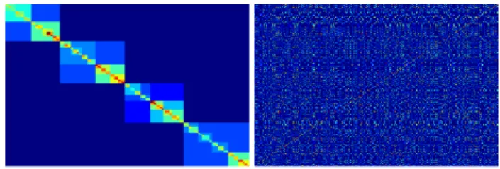
cor-relation cluster that we want to recover with a clustering al-gorithm. In Fig. 1, we display a correlation matrix from the HCBM. Notice that in practice one does not observe the hier-archical block diagonal structure displayed in the left picture, but a correlation matrix similar to the one displayed in the right picture which is identical to the left one up to a permuta-tion of the data. The HCBM defines a set of nested partipermuta-tions
P ={P0⊇P1⊇. . .⊇Ph}for someh∈[1, N], whereP0
is the trivial partition, the partitionsPk ={C
(k) 1 , . . . , C (k) lk }, and Flk i=1C (k) i = {X1, . . . , XN}. For all 1 ≤ k ≤ h,
we define ρk and ρk such that for all 1 ≤ i, j ≤ N, we
have ρk ≤ ρij ≤ ρk when C(k)(Xi) = C(k)(Xj) and
C(k+1)(X
i)6=C(k+1)(Xj), i.e.ρkandρkare the minimum
and maximum correlation respectively within all the clusters
Ci(k)in the partitionPkat depthk. In order to have a proper
nested correlation hierarchy, we must haveρk < ρk+1for all
k. Depending on the context, it can be a Spearman or Pearson
correlation matrix.
Figure 1: (left) hierarchical correlation block model; (right) observed correlation matrix (following the HCBM) identical to the left one up to a permutation of the data
Without loss of generality and for ease of demonstration we will consider the one-level HCBM withKblocks of size n1, . . . , nKsuch thatP
K
i=1ni =N. We explain later how to
extend the results to the general HCBM. We also consider the associated distance matrixd, wheredij =
1−ρij
2 . In practice,
clustering methods are applied on statistical estimates of the distance matrixd, i.e. ondˆ
ij=dij+ij, whereijare noises
resulting from the statistical estimation of correlations.
3
Clustering methods
3.1
Algorithms of interest
Many paradigms exist in the literature for clustering data. We consider in this work only hard (in opposition to soft) cluster-ing methods, i.e. algorithms produccluster-ing partitions of the data (in opposition to methods assigning several clusters to a given data point). Within the hard clustering family, we can classify for instance these algorithms in hierarchical clustering meth-ods (yielding nested partitions of the data) and flat clustering methods (yielding a single partition) such ask-means.
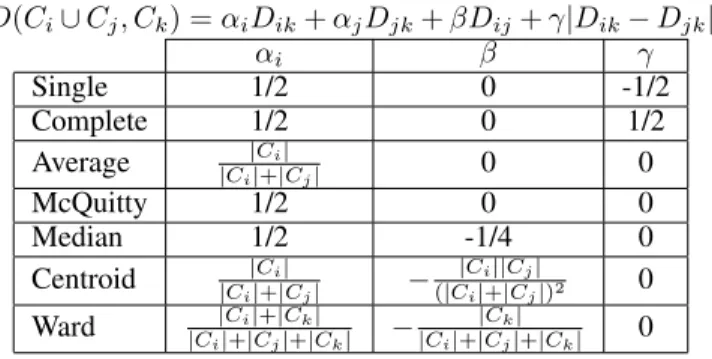
We will consider the infinite Lance-Williams family which further subdivides the hierarchical clustering since many of the popular algorithms such as Single Linkage, Complete Linkage, Average Linkage (UPGMA), McQuitty’s Linkage (WPGMA), Median Linkage (WPGMC), Centroid Linkage (UPGMC), and Ward’s method are members of this family (cf. Table 1 [Murtagh and Contreras, 2012]). It will allow us a more concise and unified treatment of the consistency proofs for these algorithms. Interesting and recently designed hierar-chical agglomerative clustering algorithms such as Hausdorff Linkage [Basaltoet al., 2007] and Minimax Linkage [Aoet al., 2005] do not belong to this family [Bien and Tibshirani,
2011], but their linkage functions share a convenient property for cluster separability.
Table 1: Many well-known hierarchical agglomerative clus-tering algorithms are members of the Lance-Williams family, i.e. the distance between clusters can be written:
D(Ci∪Cj, Ck) =αiDik+αjDjk+βDij+γ|Dik−Djk| αi β γ Single 1/2 0 -1/2 Complete 1/2 0 1/2 Average |Ci| |Ci|+|Cj| 0 0 McQuitty 1/2 0 0 Median 1/2 -1/4 0 Centroid |Ci| |Ci|+|Cj| − |Ci||Cj| (|Ci|+|Cj|)2 0 Ward |Ci|+|Ck| |Ci|+|Cj|+|Ck| − |Ck| |Ci|+|Cj|+|Ck| 0
3.2
Separability conditions for clustering
In our context the distances between the points we want to cluster are random and defined by the estimated correlations. However by definition of the HCBM, each pointXibelongs
to exactly one cluster C(k)(X
i)at a given depthk, and we
want to know under which condition on the distance matrix we will find the correct clusters defined byPk. We call these
conditions the separability conditions. A separability condi-tion for the pointsX1, . . . , XN is a condition on the distance
matrix of these points such that if we apply a clustering pro-cedure whose input is the distance matrix, then the algorithm yields the correct clusteringPk = {C
(k) 1 , . . . , C
(k)
lk }, . For
example, for{X1, X2, X3}if we haveC(X1) = C(X2) 6=
C(X3)in the one-level two-block HCBM, then a separability
condition isd1,2< d1,3andd1,2< d2,3.
Separability conditions are deterministic and depend on the algorithm used for clustering. They are generic in the sense that for any sets of points that satisfy the condition the algo-rithm will separate them in the correct clusters. In the Lance-Williams algorithm framework [Chen and Van Ness, 1996], they are closely related to “space conserving” properties of the algorithm and in particular on the way the distances be-tween clusters change during the clustering process.
Space-conserving algorithms
In [Chen and Van Ness, 1996], the authors define what they call a semi-space-conserving algorithm.
Definition 1(Semi-space-conserving algorithms). An algo-rithm is semi-space-conserving if for all clustersCi,Cj, and
Ck,
D(Ci∪Cj, Ck)∈[min(Dik, Djk),max(Dik, Djk)]
Among the Lance-Williams algorithms we study here, Sin-gle, Complete, Average and McQuitty algorithms are semi-space-conserving. Although Chen and Van Ness only con-sidered Lance-Williams algorithms the definition of a space conserving algorithm is useful for any agglomerative hier-archical algorithm. An alternative formulation of the semi-space-conserving property is:
Definition 2 (Space-conserving algorithms). A linkage ag-glomerative hierarchical algorithm is space-conserving if
Dij ∈
min
x∈Ci,y∈Cjd(x, y),x∈Ci,ymax∈Cjd(x, y)
.
Such an algorithm does not “distort” the space when points are clustered which makes the sufficient separability condi-tion easier to get. For these algorithms the separability con-dition does not depend on the size of the clusters.
The following two propositions are easy to verify.
Proposition 1. The semi-space-conserving Lance-Williams algorithms are space-conserving.
Proposition 2. Minimax linkage and Hausdorff linkage are space-conserving.
For space-conserving algorithms we can now state a suffi-cient separability condition on the distance matrix.
Proposition 3. The following condition is a separability con-dition for space-conserving algorithms:
max 1≤i,j≤N C(i)=C(j) d(Xi, Xj) < min 1≤i,j≤N C(i)6=C(j) d(Xi, Xj) (S1)
The maximum distance is taken over any two points in a same cluster (intra) and the minimum over any two points in differ-ent clusters (inter).
Proof. Consider the set{ds
ij}of distances between clusters
afterssteps of the clustering algorithm (therefore{d0
ij}is the
initial set of distances between the points). Denote{ds inter}
(resp.{ds
intra}) the sets of distances between subclusters
be-longing to different clusters (resp. the same cluster) at step
s. If the separability condition is satisfied then we have the
following inequalities: mind0intra ≤maxd
0 intra<mind 0 inter ≤maxd 0 inter (S2) Then the separability condition implies that the separability condition S2 is verified for all stepsbecause after each step
the updated intra distances are in the convex hull of the intra distances of the previous step and the same is true for the inter distances. Moreover since S2 is verified after each step, the algorithm never links points from different clusters and the
proposition entails.
Ward algorithm
The Ward algorithm is a space-dilating Lance-Williams algo-rithm: D(Ci ∪Cj, Ck) > max(Dik, Djk). This is a more
complicated situation because the structure
mindinter <maxdinter<mindintra<maxdintra
is not necessarily preserved under the conditionmaxd0
inter<
mind0
intra. Points which are not clustered move away from
the clustered points. Outliers, which will only be clustered at the very end, will end up close to each other and far from the clustered points. This can lead to wrong clusters. Therefore a generic separability condition for Ward needs to be stronger and account for the distortion of the space. Since the distor-tion depends on the number of steps the algorithm needs, the separability condition depends on the size of the clusters.
Proposition 4(Separability condition for Ward). The sepa-rability condition for Ward reads:
n[maxd0intra−mind
0 intra]<[mind 0 inter−mind 0 intra]
Proof. LetAandBbe two subsets of theN points of sizea
andbrespectively. Then D(A, B) = ab a+b 2 ab X i∈A j∈B dij− 1 a2 X i∈A i0∈A dii0− 1 b2 X j∈B j0∈B djj0
is a linkage function for the Ward algorithm. To ensure that the Ward algorithm will never merge the wrong subsets it is sufficient that for any setsAandBin a same cluster, andA0,
B0in different clusters, we have:
D(A, B)< D(A0, B0).
Since
(
D(A, B)≤n(maxd0intra−mind
0
intra) + mind
0
intra−1 D(A0, B0)≥(mind0inter−maxd
0
intra) + maxd
0
intra−1
we obtain the condition:
n(maxd0 intra−mind 0 intra)<mind 0 inter−mind 0 intra. k-means
The k-means algorithm is not a linkage algorithm. For the
k-means algorithm we need a separability condition that
en-sures that the initialization will be good enough for the al-gorithm to find the partition. In [Ryabko, 2010] (Theorem 1), the author proves the consistency of the one-step farthest-point initializationk-means [Katsavounidiset al., 1994] with
a distributional distance for clustering processes. The separa-bility condition S1 of Proposition 3 is sufficient fork-means.
4
Consistency of well-known clustering
algorithms
In the previous section we have determined configurations of points such that the clustering algorithm will find the right partition. The proof of the consistency now relies on showing that these configurations are likely. In fact the probability that our points fall in these configurations goes to1asT → ∞.
The precise definition of what we mean by consistency of an algorithm is the following:
Definition 3 (Consistency of a clustering algorithm). Let
(Xt
1, . . . , XNt),t= 1, . . . , T, beN univariate random
vari-ables observedT times. A clustering algorithmAis consis-tent with respect to the Hierarchical Correlation Block Model (HCBM) defining a set of nested partitionsP if the proba-bility that the algorithmA recovers all the partitions inP
converges to1whenT → ∞.
As we have seen in the previous section the correct cluster-ing can be ensured if the estimated correlation matrix verifies some separability condition. This condition can be guaran-teed by requiring the error on each entry of the matrix RˆT to be smaller than the contrast, i.e. ρ1−ρ0
2 , on the
theoreti-cal matrixR. There are classical results on the concentration properties of estimated correlation matrices such as:
Theorem 1(Concentration properties of the estimated
corre-lation matrices [Liuet al., 2012a]). IfΣandΣˆ are the pop-ulation and empirical Spearman correlation matrix respec-tively, then with probability at least1− 1
T2, forN ≥ 24 logT+2, we have kΣˆ−Σk∞≤24 r logN T
The concentration bounds entails that ifT log(N)then the clustering will find the correct partition because the clus-ters will be sufficiently separated with high probability. In financial applications of clustering, we need the error on the estimated correlation matrix to be small enough for relatively short time-windows. However there is a dimensional depen-dency of these bounds [Tropp, 2015] that make them unin-formative for realistic values ofN andT in financial appli-cations, but there is hope to improve the bounds using the special structure of HCBM correlation matrices.
4.1
From the one-level to the general HCBM
To go from the one-level HCBM to the general case we need to get a separability condition on the nested partition model. For both space-conserving algorithms and the Ward algo-rithm, this is done by requiring the corresponding separability condition for each level of the hierarchy.
For all1 ≤k ≤ h, we definedk anddk such that for all
1 ≤ i, j ≤N, we havedk ≤ dij ≤ dk whenC(k)(Xi) =
C(k)(X
j)andC(k+1)(Xi)=6 C(k+1)(Xj). Notice thatdk=
(1−ρk)/2anddk= (1−ρk)/2.
Proposition 5. [Separability condition for space-conserving algorithms in the case of nested partitions] The separability condition reads:
dh< dh−1< . . . < dk+1< dk< . . . < d1.
This condition can be guaranteed by requiring the error on each entry of the matrixΣˆ to be smaller than the lowest con-trast. Therefore the maximum error we can have for space-conserving algorithms on the correlation matrix is
kΣ−Σˆk∞<min
k
ρk+1−ρk
2 .
Proposition 6. [Separability condition for the Ward algo-rithm in the case of nested partitions] Letnk be the size of
the largest cluster at the levelkof the hierarchy. The separability condition reads:
∀k∈ {1, . . . , h}, nk(dk−dh)< dk−1−dh
Therefore the maximum error we can have for space-conserving algorithms on the correlation matrix is
kΣ−Σˆk∞<min
k
ρh−ρk−1−nk(ρh−ρk)
1 + 2nk
,
wherenkis the size of the largest cluster at the levelkof the
hierarchy.
We finally obtain consistency for the presented algorithms with respect to the HCBM from the previous concentration results.
5
Empirical rates of convergence
We have shown in the previous sections that clustering cor-related random variables is consistent under the hierarchical correlation block model. This model is supported by many empirical studies [Mantegna, 1999] where the authors scruti-nize time series of returns for several asset classes. However, it was also noticed that the correlation structure is not fixed and tends to evolve through time. This is why, besides being consistent, the convergence of the methodology needs to be fast enough for the underlying clustering to be accurate. For now, theoretical bounds such as the ones obtained in Theo-rem 1 are uninformative for realistic values ofN andT. For
example, for N = 265 and T = 2500(roughly 10 years of historical daily returns) with a separation between clusters of d = 0.2, we are confident with probability greater than
1−2N2e−T d2/24≈ −2176that the clustering algorithm has
recovered the correct clusters. These bounds will eventually converge to0 with rateOP(
√
logN /√T). In addition, the convergence rates also depend on many factors, e.g. the num-ber of clusters, their relative sizes, their separations, whose influence is very specific to a given clustering algorithm, and thus difficult to consider in a theoretical analysis.
To get an idea of the minimal amount of data one should use in applications to be confident with the clustering results, we suggest to design realistic simulations of financial time series and determine the sample critical size from which the clustering approach “always” recovers the underlying model. We illustrate such an empirical study in the following section.
5.1
Financial time series models
For the simulations, implementation and tutorial available atwww.datagrapple.com/Tech, we will consider two
models:
• The standard but debated model of quantitative finance,
the Gaussian random walk model whose increments are realizations from aN-variate Gaussian:X ∼ N(0,Σ).
The Gaussian model does not generate heavy-tailed behavior (strong unexpected variations in the price of an asset) which can be found in many asset returns [Cont, 2001] nor does it generate tail-dependence (strong variations tend to occur at the same time for several assets). This oversimplified model provides an empirical convergence rate for clustering that is unlikely to be exceeded on real data.
• The increments are realizations from aN-variate Stu-dent’s t-distribution, with degree of freedom ν = 3:
X ∼tν(0,ν−ν2Σ).
TheN-variate Student’st-distribution (ν = 3) captures both the heavy-tailed behavior (since marginals are univariate Stu-dent’s t-distribution with the same parameter ν = 3) and the tail-dependence. It has been shown that this distribution yields a much better fit to real returns than the Gaussian dis-tribution [Hu and Kercheval, 2010].
The Gaussian andt-distribution are parameterized by a
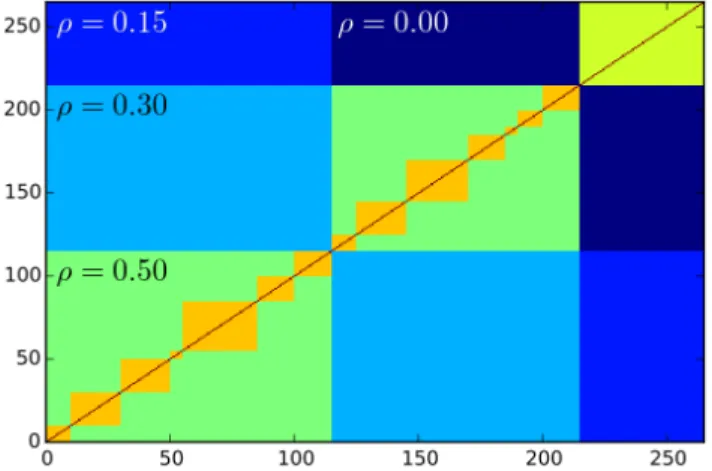
co-variance matrixΣ. We defineΣsuch that the underlying cor-relation matrix has the structure depicted in Figure 2. This correlation structure is inspired by the real correlations be-tween credit default swap assets in the European “investment
Figure 2: Illustration of the correlation structure used for sim-ulations: European assets (numbered0, . . . ,214) are
subdi-vided into2 clusters which are themselves subdivided into 7clusters each; Japanese assets (numbered215. . . ,264) are
weakly correlated to the European markets: ρ = 0.15with “investment grade” assets,ρ= 0.00with “high-yield” assets grade”, European “high-yield” and Japanese markets. More precisely, this correlation matrix allows us to simulate the re-turns time series forN = 265assets divided into
• a “European investment grade” cluster composed of115 assets, subdivided into
– 7 industry-specific clusters of sizes 10, 20, 20, 5, 30, 15, 15; the pairwise correlation inside these 7 clusters is0.7;
• a “European high-yield” cluster composed of100assets, subdivided into
– 7industry-specific clusters of sizes 10, 20, 25, 15, 5, 10, 15; the pairwise correlation inside these 7 clusters is0.7;
• a “Japanese” cluster composed of50assets whose pair-wise correlation is0.6.
We can then sample time series from these two models.
5.2
Experiment: Recovering the initial clusters
For each model, for everyTranging from10to500, we sam-ple L = 103 datasets ofN = 265 time series with length
T from the model. We count how many times the clustering
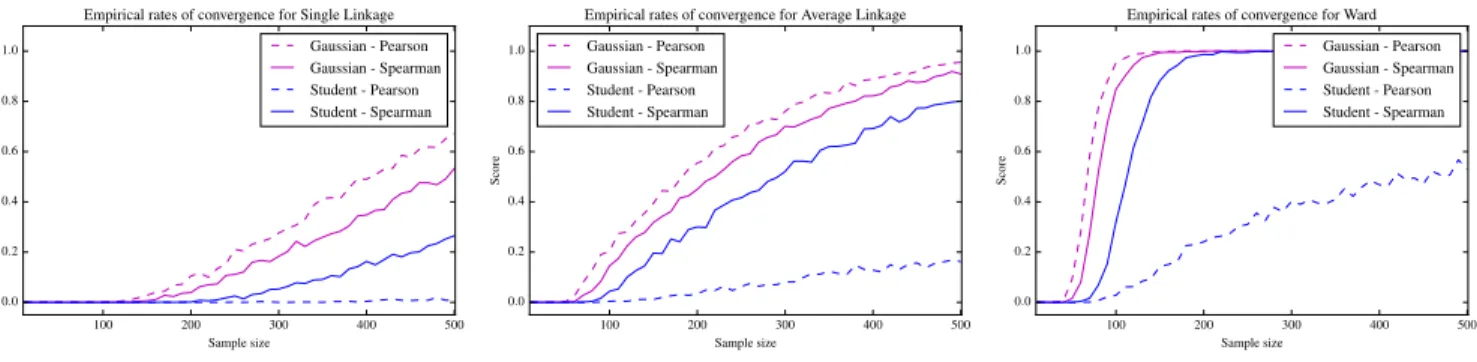
methodology (here, the choice of an algorithm and a corre-lation coefficient) is able to recover the underlying clusters defined by the correlation matrix. In Figure 3, we display the results obtained usingSingle Linkage(motivated in Mantegna et al.’s research [Mantegna and Stanley, 1999] by the
metric space hypothesis and the related subdominant ultra-metric given by the minimum spanning tree),Average Link-age(which is used to palliate against the unbalanced effect of
Single Linkage, yet unlike Single Linkage, it is sensitive to monotone transformations of the distancesdij) and theWard
method leveraging either the Pearson correlation coefficient
100 200 300 400 500 Sample size 0.0 0.2 0.4 0.6 0.8 1.0 Score
Empirical rates of convergence for Single Linkage Gaussian - Pearson Gaussian - Spearman Student - Pearson Student - Spearman 100 200 300 400 500 Sample size 0.0 0.2 0.4 0.6 0.8 1.0 Score
Empirical rates of convergence for Average Linkage Gaussian - Pearson Gaussian - Spearman Student - Pearson Student - Spearman 100 200 300 400 500 Sample size 0.0 0.2 0.4 0.6 0.8 1.0 Score
Empirical rates of convergence for Ward Gaussian - Pearson Gaussian - Spearman Student - Pearson Student - Spearman
Figure 3: Single Linkage (left), Average Linkage (mid), Ward method (right) are used for clustering the simulated time series; Dashed lines represent the ratio of correct clustering over the number of trials when using Pearson coefficient, solid lines for the Spearman one; Magenta lines are used when the underlying model is Gaussian, blue lines for thet-distribution
5.3
Conclusions from the empirical study
As expected, the Pearson coefficient yields the best results when the underlying distribution is Gaussian and the worst when the underlying distribution is heavy-tailed. For such elliptical distributions, rank-based correlation estimators are more relevant [Liuet al., 2012b; Han and Liu, 2013].
Con-cerning clustering algorithm convergence rates, we find that Average Linkage outperforms Single Linkage for T N
andT ' N. One can also notice that both Single Linkage and Average Linkage have not yet converged after 500 real-izations (roughly 2 years of daily returns) whereas the Ward method, which is not mainstream in the econophysics liter-ature, has converged after 250 realizations (about a year of daily returns). Its variance is also much smaller. Based on this empirical study, a practitioner working with N = 265 assets whose underlying correlation matrix may be similar to the one depicted in Figure 2 should use the Ward + Spearman methodology on a sliding window of lengthT = 250.
6
Discussion
In this contribution, we only show consistency with respect to a model motivated by empirical evidence. All models are wrongand this one is no exception to the rule: random walk
hypothesis, real correlation matrices are not that “blocky”. We identified several theoretical directions for the future:
• The theoretical concentration bounds are not sharp enough for usual values of N, T. Since the intrinsic
dimension of the correlation matrices in the HCBM is low, there might be some possible improvements [Tropp, 2015].
• “Space-conserving”, “space-dilating” is a coarse
classi-fication that does not allow to distinguish between sev-eral algorithms with different behaviors. Though Single Linkage (which is nearly “space-contracting”) and Aver-age LinkAver-age have different convergence rates as shown by the empirical study, they share the same theoretical bounds.
And also directions for experimental studies:
• It would be interesting to study spectral clustering tech-niques which are less greedy than the hierarchical
clus-Figure 4: Heatmap encoding the ratio of correct clustering over the number of trials for the Ward + Spearman method-ology as a function ofρandT; underlying model is a
Gaus-sian distribution parameterized by a 2-block-uniform-ρ cor-relation matrix; red color represents a perfect and systematic recovering of the underlying two clusters, deep blue encodes 0 correct clustering; notice the clear-cut isoquants
tering algorithms. In [Tumminelloet al., 2007], authors
show that they are less stable with respect to statistical uncertainty than hierarchical clustering. Less stability may imply a slower convergence rate.
• We notice that there are isoquants of clustering accuracy for many sets of parameters, e.g. (N, T),(ρ, T). Such isoquants are displayed in Figure 4. Further work may aim at characterizing these curves. We can also observe in Figure 4 that forρ≤0.08, the critical value forT
ex-plodes. It would be interesting to determine this asymp-totics asρtends to 0.
Finally, we have provided a guideline to help the prac-titioner set the critical window-size T for a given
cluster-ing methodology. One can also investigate which consistent methodology provides the correct clustering the fastest. How-ever, much work remains to understand the convergence be-haviors of clustering algorithms on financial time series.
References
[Aoet al., 2005] Sio Iong Ao, Kevin Yip, Michael Ng,
David Cheung, Pui-Yee Fong, Ian Melhado, and Pak C Sham. Clustag: hierarchical clustering and graph methods for selecting tag snps. Bioinformatics, 21(8):1735–1736,
2005.
[Balakrishnanet al., 2011] Sivaraman Balakrishnan, Min
Xu, Akshay Krishnamurthy, and Aarti Singh. Noise thresholds for spectral clustering. InAdvances in Neural Information Processing Systems, pages 954–962, 2011.
[Basaltoet al., 2007] Nicolas Basalto, Roberto Bellotti,
Francesco De Carlo, Paolo Facchi, Ester Pantaleo, and Saverio Pascazio. Hausdorff clustering of financial time series. Physica A: Statistical Mechanics and its Applica-tions, 379(2):635–644, 2007.
[Bien and Tibshirani, 2011] Jacob Bien and Robert Tibshi-rani. Hierarchical clustering with prototypes via minimax linkage. Journal of the American Statistical Association,
106(495):1075–1084, 2011.
[Borysovet al., 2014] Petro Borysov, Jan Hannig, and
JS Marron. Asymptotics of hierarchical clustering for growing dimension. Journal of Multivariate Analysis,
124:465–479, 2014.
[Chen and Van Ness, 1996] Zhenmin Chen and John W Van Ness. Space-conserving agglomerative algorithms.
Journal of classification, 13(1):157–168, 1996.
[Cont, 2001] Rama Cont. Empirical properties of asset re-turns: stylized facts and statistical issues. 2001.
[Han and Liu, 2013] Fang Han and Han Liu. Optimal rates of convergence for latent generalized correlation matrix estimation in transelliptical distribution. arXiv preprint arXiv:1305.6916, 2013.
[Hartigan, 1981] John A Hartigan. Consistency of single linkage for high-density clusters.Journal of the American Statistical Association, 76(374):388–394, 1981.
[Hu and Kercheval, 2010] Wenbo Hu and Alec N Kercheval. Portfolio optimization for student t and skewed t returns.
Quantitative Finance, 10(1):91–105, 2010.
[Katsavounidiset al., 1994] Ioannis Katsavounidis, C-C
Jay Kuo, and Zhen Zhang. A new initialization technique for generalized Lloyd iteration.Signal Processing Letters, IEEE, 1(10):144–146, 1994.
[Khaleghiet al., 2012] Azadeh Khaleghi, Daniil Ryabko,
J´er´emie Mary, and Philippe Preux. Online clustering of processes. InInternational Conference on Artificial Intel-ligence and Statistics, pages 601–609, 2012.
[Kleinberg, 2003] Jon Kleinberg. An impossibility theorem for clustering. Advances in neural information processing systems, pages 463–470, 2003.
[Krishnamurthyet al., 2012] Akshay Krishnamurthy,
Sivaraman Balakrishnan, Min Xu, and Aarti Singh. Efficient active algorithms for hierarchical clustering.
International Conference on Machine Learning, 2012.
[Liuet al., 2012a] Han Liu, Fang Han, Ming Yuan, John
Lafferty, Larry Wasserman, et al. High-dimensional semi-parametric gaussian copula graphical models. The Annals of Statistics, 40(4):2293–2326, 2012.
[Liuet al., 2012b] Han Liu, Fang Han, and Cun-hui Zhang.
Transelliptical graphical models. InAdvances in Neural Information Processing Systems, pages 809–817, 2012.
[Mantegna and Stanley, 1999] Rosario N Mantegna and H Eugene Stanley. Introduction to econophysics: corre-lations and complexity in finance. Cambridge university
press, 1999.
[Mantegna, 1999] Rosario N Mantegna. Hierarchical struc-ture in financial markets. The European Physical Journal B-Condensed Matter and Complex Systems, 11(1):193–
197, 1999.
[Martiet al., 2015] Gautier Marti, Philippe Very, Philippe
Donnat, and Frank Nielsen. A proposal of a methodologi-cal framework with experimental guidelines to investigate clustering stability on financial time series. In14th IEEE International Conference on Machine Learning and Appli-cations, ICMLA 2015, Miami, FL, USA, December 9-11, 2015, pages 32–37, 2015.
[Murtagh and Contreras, 2012] Fionn Murtagh and Pedro Contreras. Algorithms for hierarchical clustering: an overview. Wiley Interdisciplinary Reviews: Data Mining and Knowledge Discovery, 2(1):86–97, 2012.
[Pollard and others, 1981] David Pollard et al. Strong con-sistency ofk-means clustering. The Annals of Statistics,
9(1):135–140, 1981.
[Ryabko, 2010] D. Ryabko. Clustering processes. InProc. the 27th International Conference on Machine Learning (ICML 2010), pages 919–926, Haifa, Israel, 2010.
[Terada, 2013] Yoshikazu Terada. Strong consistency of fac-torial k-means clustering. Annals of the Institute of Statis-tical Mathematics, 67(2):335–357, 2013.
[Terada, 2014] Yoshikazu Terada. Strong consistency of re-duced k-means clustering.Scandinavian Journal of Statis-tics, 41(4):913–931, 2014.
[Tolaet al., 2008] Vincenzo Tola, Fabrizio Lillo, Mauro
Gal-legati, and Rosario N Mantegna. Cluster analysis for port-folio optimization. Journal of Economic Dynamics and Control, 32(1):235–258, 2008.
[Tropp, 2015] Joel A Tropp. An introduction to matrix con-centration inequalities. arXiv preprint arXiv:1501.01571,
2015.
[Tumminelloet al., 2007] Michele Tumminello, Fabrizio
Lillo, and Rosario N Mantegna. Kullback-leibler distance as a measure of the information filtered from multivariate data.Physical Review E, 76(3):031123, 2007.
[Von Luxburget al., 2008] Ulrike Von Luxburg, Mikhail
Belkin, and Olivier Bousquet. Consistency of spectral clustering.The Annals of Statistics, pages 555–586, 2008.