Learning-based Nonlinear Model Predictive
Control
?
D. Limon∗J. Calliess∗∗J.M. Maciejowski∗∗
∗Universidad de Sevilla. [email protected]
∗∗University of Cambridge.{jpc73,jmm}@cam.ac.uk
Abstract
This paper presents stabilizing Model Predictive Controllers (MPC) in which prediction models are inferred from experimental data of the inputs and outputs of the plant. Using a nonparametric machine learning technique called LACKI, the estimated (possibly nonlinear) model function together with an estimation of H¨older constant is provided. Based on these, a number of predictive controllers with stability guaranteed by design are proposed. Firstly, the case when the prediction model is estimated off-line is considered and robust stability and recursive feasibility is ensured by using tightened constraints in the optimisation problem. This controller has been extended to the more interesting and complex case: the online learning of the model, where the new data collected from feedback is added to enhance the prediction model. An on-line learning MPC based on a double sequence of predictions is proposed.
Keywords:MPC; Data-based control; Machine learning; Input-to-state stability. 1. INTRODUCTION
Model-based control design, and particularly Model Predictive Control (MPC), rely on the availability of an accurate descrip-tion of the plant. When a model of the plant dynamics is un-available a priori, machine learning methods can be employed to devise such models automatically from observational data. The objective of this paper is to design a predictive controller based on such learning methods. Here, the learning method should be flexible enough to learn rich classes of dynamical systems, while at the same time, offer bounds on its predictive performance.
The latter is important in the predictive control setting if one wishes to give guarantees on the performance and feasibility of the learning-based controller.
Motivated by these desiderata, previous work on learning-based MPC Canale et al. (2014) has utilised Nonlinear Set Member-ship (NSM) methods Sukharev (1978); Milanese and Novara (2004) for learning. These methods are capable of learning any Lipschitz continuous function with a known, given Lipschitz constant and provide bounds around the predictions of the learned model. In their data-based Nonlinear MPC (NMPC) method, Canale et al. (2014) presuppose a bound on the worst-case estimation error for the data set which they call the radius of information. Assuming that a stabilizing nominal MPC for the estimated prediction model has been designed, the authors prove that this controller is robustly stable. However, to do so, the authors not only need to assume that the bound on the Lipschitz constant and the radius of information are known, but they also assume that the nonlinear MPC optimization problem
? The authors would like to ackowledge to the Spanish MINECO Grant
PRX15-00300 and projects DPI2013-48243-C2-2-R and DPI2016-76493-C3-1-R as well as to the Engineering and Physical Research Council, grant no. EP/J012300/1 for funding this work.
happens to be recursively feasible, in spite of the prediction errors.
An alternative approach to learning-based MPC that is more independent of the concrete learning paradigm was proposed in Aswani et al. (2013). Here, the authors assumed that the true model was given by a linear model plus a function to be learned. The amplitude of the latter function had to be limited and small since it was considered to be an exogenous disturbance for the robust design of the linear robust MPC. The trained nonlinear model only entered the cost function while the nominal linear model was considered for the constraint satisfaction. Thus, the resulting feasibility region is convex, which allows the authors to derive robust stability provided that learning methods are employed that provide bounds around their predictions. Since the uncertainty must enclose the estimation error and the mismatch between the linear and nonlinear dynamics, the resulting design might be quite conservative Furthermore, the stability proof relies on the convexity of the constraints of the optimisation problem which cannot be extended to nonlinear models where convexity may not hold, requiring appropriate stability conditions.
In our paper, we improve on this existing state of affairs in several ways. Firstly, we propose to utilise nonlinear prediction models based on a recent improvement on NSM learning ap-proach called LACKI Calliess (2016) which estimates Lipschitz constants from the data while still offering worst-case pre-diction error bounds. Secondly, we design our learning-based NMPC approach in a manner that ensures robust stability and recursive feasibility w.r.t. the estimation error. Thirdly, we also consider the online learning setting where the learning model is updated repeatedly during the runtime of the controller. Using a similar idea to Aswani et al. (2013), two predicted trajectories are entertained in the optimisation problem: one is based on the offline learned model and guarantees the robust constraint satisfaction while the second is calculated by the on-line learn-ing method and it is used for the calculation of the cost
func-tion. Since in our case the prediction models are nonlinear and the resulting optimization problem is non-convex, the proof of Aswani et al. (2013) cannot be used for our case. Instead, we have derived input-to-state stability under mild assumptions on the estimator.
The rest of the paper is structured as follows: Following this introduction, a brief rehearsal of some of the learning methods this work could build upon is provided, followed by an intro-duction to the data-based control problem and a derivation of our predictive controller.
In the first part of the remainder of the paper, the controller is based on a fully trained learning model based on data that has been collected offline. That is, the sample is collected once, before control is attempted, on the basis of which the model is trained, without further updates during the operation of the controller. The LACKI method provides the estimated prediction model together with an estimation of the Lipschitz constant. Based on these ingredients and on the bound of the worst-case estimation error, a NMPC is proposed such that robust stability and recursive feasibility is ensured by design. In the second part of the paper, we lift this assumption and the case of online learning. Here the sample is repeatedly updated during the runtime of the controller in order to learn a contin-uously more accurate model of the plant and improve control performance. The previous data-based MPC controller has been extended to the online learning data-based NMPC, which al-lows us to use a continuously updated prediction model which provides better closed loop performance while robust stability and recursive feasibility are still guaranteed. The proofs have been omitted due to the lack of space. A preliminary version of the proofs can be found in the technical report Limon et al. (2017).
Notation and terminology
Let a, b be two column vectors and (a, b) denote the vector [aT, bT]T. Given two sets A, B, the Minkowski sumA⊕B is defined as the set {a + b : a ∈ A, b ∈ B} and the Pontryagin difference A B is defined as the set {c : c+
b ∈ A, ∀b ∈ B}. The set of the integers contained in the interval [a, b] with b ≥ a is denoted as Ia,b. A function
θ : R≥0 → R≥0 is a K-function if it is strictly increasing
and θ(0) = 0. If aK-function is such that lim
s→∞θ(s) = ∞
then it is called a K∞-function. Remember, a pseudo-metric
dX(·,·) : X2 →
R on a space X is a symmetric, positive
mapping that adheres to the triangle-inequality. In contrast, to full metrics, a pseudo-metric does not require definiteness. That is, it is possible that dX(x, x0) = 0even ifx6=x0. A mapping
f :X→Ybetween pseudo-metric spaces(X,dX)and(Y,dY) is H¨older continuous with H¨older constant Land exponent p
if dY(f(x), f(x0)) ≤ LdX(x, x0)p,∀x, x0 ∈ X. The smallest
H¨older constant off will be denoted byL∗.
2. LEARNING WITH WORST-CASE PREDICTION BOUNDS
In this work, we will design a controller whose prediction model is inferred (i.e. learned) from data employing machine learning (i.e. regression) techniques. As the controller is in-tended to come with robustness guarantees, it is important that the predictions of the learned model come with deterministic
worst-case prediction error bounds. This limits our choice of learning methods to those for which such bounds are currently known.
A class of learning rules, for which this is the case, and which have been proposed in the context of control, are sometimes referred to as Kinky Inference [Calliess (2014)] which en-compass Lipschitz Interpolation [Sukharev (1978); Beliakov (2006)] and Nonlinear Set Interpolation [Milanese and Novara (2004)]. These methods will be briefly rehearsed next.
Setting. Let X, Y be two spaces endowed with (pseudo-) metrics dX : X2 →
R≥0,dY : Y2 → R≥0, respectively.
SpacesX,Ywill be referred to asinput spaceandoutput space, respectively. It will be convenient to restrict our attention to input and output spaces that are additive abelian groups and which aretranslation-invariantwith respect to their (pseudo) metrics. That is, for the input space X, we assume dX(x+
x0, x00+x0) = d(x, x00),∀x, x0, x00∈X.
For simplicity, throughout the remainder of this work, we will assume the output space is the canonical Hilbert spaceY=Rm
(m∈N)endowed with the dY(y, y0) =ky−y0k∞,∀y, y0 ∈
Y.
Letf :X→Ybe atargetorground-truthfunction we desire to learn. For our purposes, learning means regression. That is, we utilise the data to construct a computable function that allows us predict values of the target function at any given input. Assume that, at time stepn, we have access to a sample or
data setDn :={ si,f˜i
|i= 1, . . . , Nn}containingNn ∈N
(possibly erroneous) sample vectorsf˜i ∈ Yoftarget function
f at sample input si ∈ X. The sampled function values are allowed to have interval-boundedobservational error ornoise
given by a bound e : X → Rm≥0. That is, all we know is
thatf(si) ∈ Oi := [f1(si), f1(si)]×. . .×[fd(si), fd(si)] wheref
j(si) := ˜fi,j−ej(si),f(si) := ˜fi,j+ej(si)and ˜
fi,j denotes thejth component of vectorf˜i. The interpretation of these errors depends on the given application and this “noise” may be deterministic or stochastic. For instance, in the context of system identification, the sample might be based on noisy measurements of velocities and it may be due to sensor noise or may capture numerical approximation error, as well as input uncertainty Calliess (2014).
Learning.It is our aim to learn target functionf in the sense that, combining prior knowledge aboutfwith the observed data
Dn, we infer predictions ˆfn(x)of f(x) at unobservedquery inputsx /∈XDn. Here,XDn={si|i= 1. . . , Nn}refers to the
(not necessarily regular)gridof sample inputs. In our context, the evaluation ofˆfnis what we refer to as(inductive) inference orprediction. The entire functionˆfnthat is learned to facilitate
predictions is referred to as thepredictor.
A typicaldesideratumof a good predictor is that it is efficiently
computableandconverges to the target(up to the observational error given bye) in the limit of increasingly dense data sets. In our context, we will understand amachine learning algo-rithmto implement a computable function that maps a data set
In this work we will expand on the basis of the following class of predictors to perform learning as inference over unobserved function values:
Definition 1.(Kinky Inference (KI) rule ). Let R∞ := R ∪
{−∞,∞}andXbe some space endowed with a pseudo-metric
dX. Let B,B¯ : X → Y ⊆ Rm∞ denote lower- and upper bound functions, that can be specified in advance and assume
B(x)≤ B¯(x),∀x∈I⊂Xcomponent-wise. Furthermore, let
edenote a parameter that specifies a deterministic belief about the true observational error bounde. Given sample setDn, we define the predictive functions ˆfn:X→Y,vˆn:X→Rm≥0to
perform inference over function values. Forj = 1, . . . , m, their
jth output components are given by: ˆfn,j(x) :=1 2min{ ¯ Bj(x),un,j(x;L(n) } +1 2max{Bj(x),ln,j(x;L(n) }, ˆ vn,j(x) := 1 2min{ ¯ Bj(x),un,j x;L(n) } −1 2max{Bj,ln,j x;L(n) }. Here,un ·;L(n) ,ln ·;L(n)
: X → Rm are called ceiling and floor functions, respectively. Their jth component func-tions are given by
un,j x;L(n) := min i=1,...,Nn ˜ fi,j+Lj(n)dp(x, si) +ej(x) and ln,j x;L(n):= max i=1,...,Nn ˜ fi,j−Lj(n)dp(x, si)−ej(x), respectively. Herep∈R, L(n)∈Rm,∀n∈N0and functions
B,B, e¯ :X→Rm∞are parameters that have to be specified in
advance. To disable restrictions of boundedness, it is allowed to specify the upper and lower bound functions to constants ∞ or −∞, respectively. Function ˆfn is the predictor that is
to be utilised for predicting/inferring function values at unseen inputs. Function ˆvn(x)is meant to quantify the uncertainty of
predictionˆfn(x).
Note, that while generallyL(n)is a vector, we will simplify our exposition in the remainder of this paper by assuming that all its components are equal or, equivalently, that it is a real number. To provide an intuition, consider the following special case where we have access to a noise-free sampleDn and suppose the target f is a real-valued L∗−pH¨older continuous
func-tion. Observing the noise-free sample point(si, fi)constrains the set of function values f(x) to the set Si(x) = {φ ∈
Y|dY(φ, fi) ≤ L∗dX(si, x)}. Considering a set of sample points Dn, target value f(x) is constrained to lie in the in-tersection S(x) = ∩Nn
i=1Si(x). It is easy to see that the floor and ceiling functions are tight lower and upper bounds ofS(x)
withS(x) := {φ ∈ Y|ln(x;L∗) ≤ φ ≤ un(x;L∗)}. In other words, setting parameterL(n)to the best H¨older constantL∗
and bounds B = −∞,B¯ = +∞ yields a predictor ˆfn(x)
that for every queryxchooses the mid-point of the setS(x)of
those function values that can possibly be assumed by a H¨older continuous function that interpolates the observed sample. Pre-diction error ˆvn(x)simply is the radius of the set.
For the case of p = 1, this approach is known as Lipschitz interpolationBeliakov (2006); Zabinsky et al. (2003). Since a set is utilised for interpolation, the approach is also known as
Nonlinear Set InterpolationMilanese and Novara (2004).
Spec-ification of B, B¯ allows us to incorporate additional knowl-edge and constrain our set S(x) further. For instance, when
learning friction models we might incorporate the knowledge of dealing with negative functions by setting B¯ = 0, yielding
S(x) ={φ|φ≤0} ∩Ni=1n Si(x).
When choosingL(n)to coincide with a H¨older constant of the target function, one can give strong guarantees of convergence to the target as on the tightness of the prediction bounds [e.g. Calliess (2014)]. In case a H¨older constant is unknown a priori, Milanese and Novara (2004) have proposed to utilise a proxy regression model to estimate the constant from the data. Unfortunately, as far as we can tell, all convergence guarantees and uncertainty bounds are lost in the process. On the other hand, ifL(n)was chosen to a very conservatively large constant then the resulting predictor tends to overfit to the noise and hence, exhibit poor prediction performance [Calliess (2016)]. As an alternative, Calliess (2014) has proposed to set
L(n) := max i,j=1,...,NndX(si,sj)>0 ˜ fi−f˜j ∞−2¯e dX(si, sj)
where¯e := supx|e(x)|is an upper bound on the (zero-mean) noise. The resulting predictor, referred to asLACKI has been investigated by Calliess (2016). For cases where¯eis known the authors derived parameter settings for the LACKI inference rule for which the following prediction error bound was derived:
dY ˆfn(x), f(x)
∈
0,2` rpx(n) + 2¯e
. (1)
whererx(n) = mins∈Gn dX(x, s)is the distance of the query
inputx to the input data and` ∈ R, ` ≥ L∗ is any H¨older
constant of the target functionf. Note, that while the prediction errorboundstill depends on knowledge of a H¨older constant, the predictorˆfnitself only depends on the empirical estimator.
Therefore,`could be chosen conservatively large without caus-ing the predictions to be prone to overfit to observational noise Calliess (2016).
3. DATA-BASED PREDICTION MODEL
Let the manipulable inputs of the plant at sampling time step
k ∈ Nbeu(k) ∈ IRmand the controlled outputs bey(k) ∈
IRn. It is assumed that the output signal is measured and can be used to describe the model of the system by means of the followingNARXmodel of the plant
y(k+ 1) =g(x(k), u(k)) +e(k) (2) where x(k) = (y(k),· · ·, y(k−na), u(k −1),· · ·, u(k−
nb)) ∈ X := Y(na+1) ×Unb ⊂ Rnx with n
x = (na + 1)n+nbm, for some memory horizon lengthsna, nb∈N. The
signale(k)models output noise and is assumed to be confined in a compact setE. For notational convenience, we sometimes aggregate the inputs ofginto a joint inputξ:= (x, u)∈Ξ :=
X×U. So, we can writeg: Ξ→Y.
It is assumed that the origin is the equilibrium point of the system (i.e.g(0,0) = 0) where the plant must be stabilized. Furthermore, the system is subject to constraints that must be satisfied at each sampling time:
u(k)∈U, y(k)∈Y (3) whereUandYare compact sets.
(1) The pseudo-metricsdX:X×X→R≥0anddY:Y×Y→
R≥0are such that forx= (y1,· · · , yna+1,0,· · ·,0), the
following condition holds
dX(x,0)≤dY(y1,0) +· · ·dY(yna+1,0).
(2) The functiong(·), referred to asground truth function, is H¨older continuous. That is, there exists someLg >0and
p∈(0,1)such that
dY(g(x1, u), g(x2, u))≤LgdX(x1, x2)p (4)
wheredYstands for a pseudo-metric defined in the set of outputsY, anddX stands for a pseudo-metric defined in the set of the states of the model functionX=Y(na+1)×
Unb. The lowest constantL
gthat satisfies this condition is called the H¨older constant,L∗g.
In this paper we assume that the prediction model will be inferred from a set of pairs of input-output experimental data
D={(y(j), u(j))|j= 1,· · ·, ND}.
This data may be extracted from some experiments or from stored historical data of the plant.
Notice that the data set can be recast asDg = { ξ(j), y(j+ 1)
j = j0,· · ·, ND − 1}, where j0 = max(na + 1, nb). We can define ΞD := { ξ(j)
j = j0,· · ·, ND −1} and
YD := { y(j)j = j0,· · ·, ND−1} as the available inputs and output samples ofgavailable in the data.
If the required H¨older constant is not known a priori, it can be estimated from the data setD with a noise-robust version Calliess (2014, 2016) of Strongin’s method Strongin (1973). This estimate, denoted byLD, can be utilised as a parameter in thekinky inferencemethod of Calliess (2014, 2016) to obtain a predictorgˆof the ground-truthg, yielding the output prediction:
ˆ
y(k+ 1) = ˆg(x(k), u(k);LD). (5) This estimated function will be used as the prediction model in the design of a model-predictive controller that is presented in the next section. Before, this is derived however, we will conclude the present section with a brief discussion of the necessity of requiring worst-case estimation bounds of the learners in a stabilizing MPC setting.
3.1 Necessity of the worst case estimation error
In general, a nonlinear system, even in the case of no uncer-tainty and no constraints, might not be globally asymptotically stabilized, but only in a certain region. This is the case of the systems that are subject to constraints on the inputs and/or the states. These constraints can be inherent to the system to be controlled or to the control law to be used.
Model-predictive control requires repeated optimisation of the predicted control inputs subject to constraints. Therefore, in order to give guarantees on the controller’s closed-loop perfor-mance, we need to ensure recursive feasibility. That is, we need to ensure that all constraints remain satisfiable during runtime, or equivalently, to guarantee that the controlled system will not leave the controllable region. However, since our controller will be based not on the ground-truth dynamicsg, but on the learned modelgˆinferred from a sample of the ground-truth, recursive feasibility can only be guaranteed if a bound on the discrepancy betweengandgˆis known a priori and taken into account by the controller.
In this paper it is assumed that a bound for the worst-case estimation error is available.
Assumption 2. It is assumed that a bound on the error between the estimated output and the real output is known. That is, there exists an a priori prediction error boundµ >0with
dY(ˆg(x, u;LD), g(x, u) +e)≤µ (6) for allx∈Yna+1×Unb,u∈Uande∈E.
Remark 2. As explained above, if some upper bound`gof the smallest H¨older constantLgof mappinggis available then the worst-case prediction error boundµof the estimated model is can be given (cf. Eq. 1) as per
µ= 2`gRpD+ 2¯e (7) where RD = supξ∈Ξinfξ0∈Ξ
D dX(ξ, ξ
0) is the worst-case
distance of query inputs to sample inputs in the data and¯e
is the bound of the noise,¯e = supe∈EdY(e,0). If the true H¨older constant is not available, then the constant could be estimated by means of a (probabilistic) validation technique from experimental data (Alamo et al. (2015)).
4. STABILIZING OFF-LINE LEARNING BASED NMPC In this section, a model predictive controller based on predic-tion model learned from off-line data of the plant is derived. Since the prediction model is not accurate, the effect of the estimation error on the predictions must be analyzed to be taken into account in the design of the controller.
For this analysis, it is convenient to define the model of the plant in a state-space description as follows (Canale et al. (2014)):
x(k+ 1) =F(x(k), u(k)) +w(k) (8) y(k) =M x(k) (9) where F(x(k), u(k)) = (g(x(k), u(k)), y(k),· · · , y(k−na+ 1), u(k),· · ·, u(k−nb+ 1)) M= [In,0,· · · ,0] andw(k) = (e(k),0,· · · ,0).
Based on the set of data obtained offlineDand the estimated H¨older constant LD, a model gˆ(x, u;LD,D) is obtained by learning. Then we can forecast the evolution of the system along a given prediction horizon N, for a given sequence of future inputsu(k+j),j= 0,· · ·, N−1at a certain state
x(k) = (y(k),· · ·, y(k−na), u(k−1),· · · , u(k−nb)).
The output forecasted at sampling time k+j based on the information at k is denoted as yˆ(j|k). Given the regressive nature of the dynamic model, the predicted state is given by
ˆ
x(j|k) = (ˆy(j|k),· · ·,yˆ(1|k), y(k),· · · , y(k+j−na),
u(k+j−1),· · ·, u(k+j−nb)) This predicted state is derived from the recursion
ˆ
x(j+ 1|k) = ˆF(ˆx(j|k), u(k+j)) (10) where
ˆ F(ˆx(j|k), u(k+j)) = (ˆg(ˆx(j|k), u(k+j), LD), ˆ y(j|k),· · ·, y(k),· · · , y(k+j−na+ 1),· · · , u(k+j),· · · , u(k+j−nb+ 1)). This prediction model depends on the learned modelˆgand then depends on the provided data setDand the estimated H¨older constant LD, but this dependence is omitted for the sake of clarity.
Since the estimated model differs from the true dynamics of the system, there exists an error between the predicted state using the approximate model and the real state for a given sequence of future control inputs. Based on Assumption 2, the effect of the estimation error on the predictions is analyzed in the following lemma:
Lemma 3. Assume that at the sampling timekthe state of the plant isx(k)and a sequence of future control inputsu(k+i) fori∈I0,N−1is given.
Let xˆ(j|k) and yˆ(j|k) be the predicted states and outputs respectively derived from (10) for the given sequence of future control inputs and the current statex(k), i.e.xˆ(0|k) =x(k). Assume that at sampling timek+ 1, the current outputy(k+ 1) is measured, and then the current statex(k+1)is known. Based on these new measurements, an updated sequence of states and outputsxˆ(j|k+ 1)andyˆ(j|k+ 1)are predicted based on (10) withxˆ(0|k+ 1) =x(k+ 1)and the remaining sequence of the given future control inputs.
Then the error between both predictions are such that
dY(ˆy(j−1|k+ 1),yˆ(j|k))≤cj (11)
dX(ˆx(j−1|k+ 1),xˆ(j|k))≤dj (12) wherecjansdjcan be calculated from the recursion
cj=LDdpj−1
dj+1=dj+LDdpj withc1=d1=µandj∈I1,N.
Remark 4. It is easy to derive that for p = 1, the constants
cj and dj are directly calculated by the following formulas
dj= (1 +LD)j−1µ, andcj=LD(1 +LD)j−1µ.
Remark 5. It can be proved that the same result holds if the error boundµis replaced by the current value of the estimation errordY(y(k+ 1),yˆ(1|k)).
Based on the derived bounds on the prediction error, the prob-lem of robust constraint satisfaction is analyzed next. Firstly, the following balls are defined:
By(δ) ={y∈ IRn :dY(y,0)≤δ}
Bx(γ) ={x∈ IRnx :d
X(x,0)≤γ}. Then, the following set of tightened constraints is defined
Yj=Y By(dj). (13) This set is said to betightenedsinceYj⊆Yand, for any output
ycontained in the tightened sety∈Yjand for all perturbations ∆y ∈By(dj)on the output, the perturbed output is contained in the original setY, i.e.y+ ∆y ∈Y. As will be shown later, the set of tightened constraints will be useful to counteract the effect of the estimation error in the predictions Limon et al. (2002).
Therefore, the tightened setYj yields sufficient conditions on recursive robust constraint satisfaction (which can be utilised in the statement of the optimisation problems of the proposed controller later on):
Lemma 6. The setsYj are such that for ally ∈Yj and for all ∆y∈By(cj),y+ ∆y∈Yj−1.
In order to ensure that the proposed controller is feasible, the tightened set of constraints must be non-empty along the prediction horizon. This is stated in the following assumption:
Assumption 3. The prediction horizon N and the estimation error boundµare such that the setYN−1is non empty.
Then the optimization problemPN(x(k), LD,D) of the pro-posed predictive controller is the following
min u VN(x(k),u) = N−1 X i=0 `(ˆy(i|k), u(i)) +Vf(ˆx(N|k)) s.t.xˆ(0|k) =x(k) (14) ˆ x(j+ 1|k) = ˆF(ˆx(j|k), u(j)), j∈I0,N−1 (15) ˆ y(j|k) =Mxˆ(j|k) (16) u(j)∈U (17) ˆ y(j|k)∈Yj (18) ˆ x(N|k)∈Xf (19)
We require the ingredients of this optimization problem to meet the following assumption:
Assumption 4.
(1) The stage cost function `(y, u) is a continuous positive definite function for all y ∈ Y and u ∈ U such that
`(y, u)≥αy(kyk)for a certainKfunctionαy.
(2) There exists a local control lawu=κf(x), a functionVf and a pair of setsΩ, Xf ⊆ IRnxsuch that:
(a) For allx∈Ωthe following conditions hold: ˆ
F(x, κf(x))∈Ω Bx(dN)
κf(x)∈U
M x∈YN−1;
(b) Xf = Ω Bx(dN);
(c) Vf is a continuous positive definite function such that
αf(kxk)≤Vf(x)≤βf(kxk)
Vf( ˆF(x, κf(x)))−Vf(x)≤ −`(M x, κf(x)) for allx∈Xf.
The following theorem presents the main result of this paper:
Theorem 7. Assume that Assumptions 2, 3 and 4 hold for the optimization problem PN(·). Let κN(x) be the control law derived from the solution ofPN(x)applied using a receding horizon policy. Then, for any feasible initial state x(0), the system controlled by the control lawu(k) =κN(x(k))is input-to-state stable w.r.t the estimation error and the constraints are always satisfied, i.e.y(k)∈Y,∀k.
4.1 Relaxation by means of soft constraints
Our previous results were based upon knowledge of the a priori prediction boundµ. If learning is done with the LACKI method
and bounds on the H¨older constant and observational errors are given thenµcould be chosen as per(7). In practice however, cases may arise where the necessary bounds may be difficult or even impossible to know beforehand. In this case it is worth remarking that theorem 7 holds as long as the uncertainty of the closed loop trajectory is such that
dY(y(k+ 1),gˆ(x(k), u(k), LD))≤µ.ˆ
If this is not the case, as was previously discussed, the satis-faction of the hard constraints cannot be ensured in general. A sensible solution to avoid feasibility problems is to relax the constraints by considering soft constraints and design the stabilizing ingredientsXfandVfas proposed in Assumption 4 using the estimated boundµˆ.
The resulting optimization problem is the following:
min u,v N−1 X i=0 `(ˆy(i|k), u(i)) +αvi +Vf(ˆx(N|k)) s.t.xˆ(0|k) =x(k) (20) ˆ x(j+ 1|k) = ˆF(ˆx(j|k), u(j)), j∈I0,N−1 (21) ˆ y(j|k) =Mxˆ(j|k) (22) u(j)∈U (23) ˆ y(j|k)∈Yj⊕By(vj) (24) vj≥0 (25) ˆ x(N|k)∈Xf (26)
Using the results on the exact penalty functions Luenberger (1984), for a sufficiently large value of α, the derived con-troller guarantees the robust constraint satisfaction when pos-sible while the constraints are relaxed when they cannot be fulfilled. The stability of the proposed controller can be derived from Theorem 7 as long as the uncertainty of the closed loop trajectory is such thatdY(y(k+ 1),gˆ(x(k), u(k), LD))≤µ.ˆ If this is not the case then the recursive feasibility of the terminal constraint cannot be ensured in the case that the model mismatch is larger than expected. This issue can be relaxed taking into account that the terminal constraint can be removed if the terminal cost function is weighted by an appropriate positive constant λ > 0 Limon et al. (2006); Rawlings and Mayne (2009). The new optimization control problem is the following min u,v N−1 X i=0 `(ˆy(i|k), u(i)) +αvi +λVf(ˆx(N|k)) s.t. xˆ(0|k) =x(k) (27) ˆ x(j+ 1|k) = ˆF(ˆx(j|k), u(j)), j∈I0,N−1 (28) ˆ y(j|k) =Mˆx(j|k) (29) u(j)∈U (30) ˆ y(j|k)∈Yj⊕By(vj) (31) vj≥0 (32)
The resulting control law would be recursively feasible, but the stability of the closed-loop system would be potentially ensured only in a (potentially not small) neighborhood of the origin Limon et al. (2006).
5. STABILIZING ON-LINE LEARNING BASED NMPC Throughout the evolution of the controlled system, new pairs of input-output data could potentially be added to the data set, yielding to an enhanced estimation of the H¨older constant. This update could be done at each sampling time or every certain number of sampling times. This is the base of the LACKI method proposed in Calliess (2016), which allows us to get estimations of the H¨older constant that are refined at each update stage, providing an enhanced estimation of the ground-truth function.
LetD(k)denote the set of all data compiled until the sampling timekand letL(k)be the estimated H¨older constant for that set provided by the LACKI algorithm. Similarly to Aswani et al. (2013), we will use two different prediction models:
• The initial or off-line learning model: ˆ
x(k+ 1) = ˆF(x(k), u(k), L0,D0)
This model is derived off-line from the historical data
D0:=D(0)available before closing the loop (i.e. at time
k = 0) and it is assumed that a guaranteed bound on the estimation error is available. The prior model is utilised to provide guaranteed estimations of the real plant and it will be used to ensure robust constraint satisfaction.
• The updated or on-line learning model: ˆ
x(k+ 1) = ˆF(x(k), u(k), L(k),D(k))
This model may provide a probably more accurate esti-mation of the real plant, but no guarantee of the estiesti-mation error is given. Subsequently, this model will be used to enhance the closed-loop behavior of the controlled plant using the updated predictions to derive the control law. Based on these prediction models, the following optimization problemPu N(x;L0,D0, L(k),D(k))is proposed: min u,L N−1 X i=0 `(ˆyu(i|k), u(i)) +Vf(ˆxu(N|k)) s.t. xˆu(0|k) =x(k) ˆ xu(j+ 1|k) = ˆF(ˆxu(j|k), u(j), L(k),D(k)), j∈I0,N−1 ˆ yu(j|k) =Mxˆu(j|k) ˆ xs(j+ 1|k) = ˆF(ˆxs(j|k), u(j), L0,D0), j∈I0,N−1 ˆ ys(j|k) =Mxˆs(j|k) u(j)∈U ˆ ys(j|k)∈Yj ˆ xs(N|k)∈Xf
In order to derive the robust stability of the proposed controller, the following assumption on the estimation method is required
Assumption 5. There exists a certain time instantk∗such that ˆ
g(x, u, L(k),D(k))∈gˆ(x, u, L0,D0)⊕B(µ)
or equivalently,
dY(ˆg(x, u, L(k),D(k)),ˆg(x, u, L0,D0))≤µ
for allx,u.
Notice that from this assumption we have that
It can be proved that the LACKI method satisfies this assump-tion.
Based on this assumption, the following lemma can be derived:
Lemma 8. Assume that Assumption 5 holds and that at the sampling timek ≥ k∗ and consider that the state of the plant is x(k) and the sequence of future control inputs is known. Let ˆxs(j|k) and yˆs(j|k) be the predicted states and outputs respectively corresponding to the given sequence of future control inputs using the guaranteed prior model.
Assume that at sampling timek+1, the states and the outputs of the plant are predicted for the remaining sequence of the given future control inputs taking into account the measured output
y(k+ 1). Letxˆs(j|k+ 1) andyˆs(j|k+ 1)be the sequences of states and outputs predicted with the prior model and let ˆ
xu(j|k+ 1)andyˆu(j|k+ 1)be the predicted sequences using the updated model atk+ 1.
Then the errors between both predictions are such that
dX(ˆxu(j−1|k+ 1),xˆs(j|k))≤dj (33) wheredjis as defined in Lemma 3.
Based on this lemma, we are ready to state the closed-loop stability of the proposed controller
Theorem 9. Consider that Assumptions 3, 4 and 5 hold. Let
κuN(x)be the control law derived from the solution ofPNu(x) applied using a receding horizon policy. Then for all feasi-ble x(0), the system controlled by the control law u(k) =
κu
N(x(k))is input-to-state stable w.r.t to the estimation error of the LACKI model and the constraints are satisfied along the time, i.e.y(k)∈Y.
6. AN ILLUSTRATION
Most of the theoretical derivations thus far were concerned with robust MPC design in a manner such that the controller and its guarantees can be connected to learning methods such as LACKI. When using such a learning method for identifying the dynamics of the underlying plant, we expect our adaptive controller to improve its performance the more data becomes available. To illustrate this behaviour, as well as the viability of our approach in general, we will now attend to a simple example:
We simulated the discrete-time version of a torque-actuated single-pendulum with continuous-time dynamicsx˙ = a(x) +
b(x)uwherea(x) :=−glsin(x1)−mlr2x2andb(x) = m l12.
Here,x1=q, x2= ˙q∈Rare joint angle position and velocity, r= 0.01denotes a friction coefficient,g= 9.81is acceleration due to gravityl= 1is the length andm= 0.1the mass of the pendulum.
The control inputu∈[−.5, .5]applies a torque to the joint that corresponds to joint-angle acceleration. The pendulum could be controlled by application of a torque uto its pivotal point.
q = 0encodes the pendulum pointing downward andq = π
denotes the position in which the pendulum is upward. Given an initial configurationx0= [0,0]we desired to steer the state to
a terminal configurationξ= [π,0]. The bounds on the control inputs were set so that the controller cannot lift up the pendulum directly to the goal position but has to plan ahead to perform a swing up. To convert the system to a discrete-time system, we chose a first-order Euler approximation with sample time ∆ = 0.1[sec.].
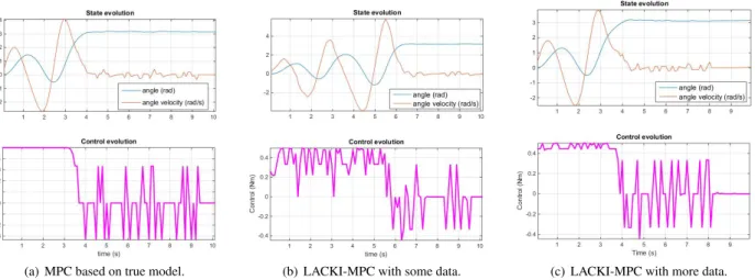
As a first test of the viability of nonlinear MPC in this setting, we designed an MPC controller as per Eq. 27-32 but where the dynamicsFˆ were set to coincide with the true dynamics. Furthermore, we chose a prediction horizon ofN = 5 time steps and, and tuned the parameters ofV andλvia linearisation around the equilibrium point. To solve the nonlinear optimi-sation problem in each step of the receding horizon control process, we employed the DIRECT global optimisation method [Jones et al. (1991)] with a computational budget of 2000 function evaluations. The resulting trajectory is depicted in Fig. 1(a). As can be seen from the plots, the controller was capable of performing the swing up and stabilising the pendulum in the up-right position (up to some jitter). We explain the remaining jitter to be an artefact of the optimisation method failing to find the global optima within the given budget.
As a first test of our learning-based MPC, we next modified the MPC, substituting the true dynamics with a LACKI predictorˆfn
trained on a data set on an even-spaced grid such that that train-ing inputs had a distance ofRDn= maxi,jksi−sjk∞= 0.6. We then repeated the simulation with this learning-based con-roller, LACKI-MPC, controlling the torques. The resulting tra-jectories are depicted in Fig.1(b). As can be seen, the controller again managed to perform the swing-up and stabilisation. How-ever, this time, most-likely due to the model inaccuracies of the trained LACKI predictor, the pendulum had to swing-back and forth repeatedly until the swing up succeeded.
To illustrate the benefit of additional data, we once more re-peated the experiment in the same setup but where LACKI was given more training data. In this second run of LACKI-MPC, the LACKI learner was trained on a finer grid with RDn = 0.4. As can be seen in Fig. 1(c), the controller managed to achieve the swing-up quicker. And, the closed-loop behaviour very closely mimicked the characteristics of those of the plant controlled by the MPC with access to the true dynamics (as per Fig. 1(a)).
7. CONCLUSIONS
In this paper, a new learning-based MPC control approach was proposed. Here control actions were based on a sequence of nonlinear MPC optimisation problems whose prediction mod-els were learned on the basis of input-output observations of the underlying plant. Several assumptions were discussed un-der which input-to-state stability of the resulting closed-loop dynamics can be proven. In contrast to some of the earlier work going in the same direction as ours, our analysis also gives guarantees on recursive feasibility of unrestricted (but typically continuous) nonlinear dynamics without having to make model assumptions that in effect limit the constraints to be convex. A crucial requirement for our guarantees to hold was that worst-case bounds around the predictions of the trained learning mod-els could be given. Providing an example of such a learning method, we considered to employ LACKI to this end [Calliess (2014, 2016)], a recently developed extension to NSM and Lipschitz interpolation methods [Sukharev (1978); Milanese and Novara (2004)] that had previously been proposed to be utilised in learning-based MPC [Canale et al. (2014)]. To illus-trate the viability of our ideas, simulations of a torque actuated pendulum were provided. Here the learning-based MPC proved capable of learning how to swing up and stabilise in the pres-ence of sufficient learning experipres-ence.
(a) MPC based on true model. (b) LACKI-MPC with some data. (c) LACKI-MPC with more data.
Figure 1. Simulations of a single pendulum. Left: Controlled by a nonlinear MPC knowing the true nonlinear dynamics. Centre: The trajectories resulting from utilising our MPC controller with soft constraints based on a coarse LACKI model trained on offline data. Right: LACKI-MPC based on a refined model.
7.1 Future work.
While the theoretical results are encouraging, a lot of avenues of further investigation remain open. For instance, we have found that in our simulations, especially in higher-dimensional sys-tems, the performance of the controller appeared to be sensitive to the computational budget and chosen nonlinear optimisation algorithm. This is especially true since the NSM and LACKI methods are not smooth. Future work will investigate alter-native optimisation algorithms that are more suitable for such function classes. From the other end, we will investigate the utilisation of smooth regression methods such as neuronal net-works or Gaussian processes [Rasmussen and Williams (2006); Kocijan and Murray-Smith (2005)] within the learning-based MPC. While we already have conducted first experiments in that regard that are encouraging, we yet have to investigate in how far these learning approaches can be proven to meet the as-sumptions required to connect to our theory. We will also study more carefully the on-line methods as well as techniques to reduce the conservativeness of the proposed approaches. Other directions are to investigate the addition of learning-oriented cost terms into the MPC objective function [e.g. similar in spirit to Alpcan (2011) ] that facilitate exploration or explic-itly encourage exploitation, giving preference to trajectories that traverse better-explored regions of state-control space over more uncertain ones.
REFERENCES
Alamo, T., Tempo, R., Luque, A., and Ramirez, D.R. (2015). Randomized methods for design of uncertain systems: Sam-ple comSam-plexity and sequential algorithms. Automatica, 52, 160–172.
Alpcan, T. (2011). Dual control with active learn-ing uslearn-ing Gaussian process regression. Arxiv preprint arXiv:1105.2211.
Aswani, A., Gonzalez, H., Sastry, S.S., and Tomlin, C. (2013). Provably safe and robust learning-based model predictive control. Automatica, 49(5), 1216–1226.
Beliakov, G. (2006). Interpolation of Lipschitz functions.
Journal of Computational and Applied Mathematics. Calliess, J.P. (2014). Conservative decision-making and
infer-ence in uncertain dynamical systems. Ph.D. thesis, Univer-sity of Oxford.
Calliess, J.P. (2016). Lazily adapted constant kinky inference for regression and nonparametric model-reference adaptive control.ArXiv pre-print, arXiv:1701.00178.
Canale, M., Fagiano, L., and Signorile, M.C. (2014). Nonlin-ear model predictive control from data: a set membership approach. International Journal of Robust and Nonlinear Control, 24(1), 123–139.
Jones, D., Peritunen, C., and Stuckman, B. (1991). Lipschitzian optimization without the Lipschitz constant.JOTA, 79(1). Kocijan, J. and Murray-Smith, R. (2005). Nonlinear Predictive
Control with a Gaussian.Lecture Notes in Computer Science 3355, Springer, 185–200.
Limon, D., Alamo, T., and Camacho, E. (2002). Input-to-state stable mpc for constrained discrete-time nonlinear systems with bounded additive uncertainties. InDecision and Con-trol, 2002, Proceedings of the 41st IEEE Conference on, volume 4, 4619–4624. IEEE.
Limon, D., Alamo, T., Salas, F., and Camacho, E.F. (2006). On the stability of MPC without terminal constraint. 42, 832– 836.
Limon, D., Callies, J., and Maciejowski, J. (2017). Stabilizing design of data-based nonlinear MPC. preliminary results. Technical report, ArXiv pre-print.
Luenberger, D.E. (1984).Linear and Nonlinear Programming. Addison-Wesley.
Milanese, M. and Novara, C. (2004). Set membership identifi-cation of nonlinear systems.Automatica.
Rasmussen, C. and Williams, C.K.I. (2006). Gaussian Pro-cesses for Machine Learning. MIT Press.
Rawlings, J.B. and Mayne, D.Q. (2009).Model Predictive Con-trol: Theory and Design. Nob-Hill Publishing, 1st edition. Strongin, R.G. (1973). On the convergence of an algorithm for
finding a global extremum.Engineering in Cybernetics. Sukharev, A. (1978). Optimal method of constructing best
uni-form approximation for functions of a certain class.Comput. Math. and Math. Phys.
Zabinsky, Z.B., Smith, R.L., and Kristinsdottir, B.P. (2003). Optimal estimation of univariate black-box Lipschitz func-tions with upper and lower bounds. Computers and Opera-tions Research.