energies
ArticleMethodology for Tuning MTDC Supervisory and
Frequency-Response Control Systems at Terminal
Level under Over-Frequency Events
Marta Haro-Larrode1,* , Maider Santos-Mugica2 , Agurtzane Etxegarai1and Pablo Eguia1
1 Department of Electrical Engineering, University of the Basque Country (Spain), 48013 Bilbao, Spain;
[email protected] (A.E.); [email protected] (P.E.)
2 Tecnalia Research and Innovation (Spain), 48160 Derio, Spain; [email protected] * Correspondence: [email protected]; Tel.:+34-630-665-715
Received: 25 April 2020; Accepted: 27 May 2020; Published: 1 June 2020
Abstract:This paper proposes a methodology for tuning a supervisory and frequency-response outer loop control system of a multi-terminal direct current (MTDC) grid designed to transmit offshore wind energy to an onshore AC grid, and to provide frequency support during over-frequency events. The control structure is based on a master–slave scheme and ensures the achievement of frequency response, with specific implementation of the UK national grid code limited-frequency sensitive (LFSM) and frequency-sensitive (FSM) modes. The onshore AC grid is modelled with an equivalent frequency-response model to simulate the onshore AC grid dynamics under frequency deviations. The main innovation of this paper is the development of a methodology for tuning simultaneously two hierarchical levels of a MTDC coordinated control structure, i.e., the MTDC supervisor, given by the active power set point for slave terminal, and the slope of frequency-response functions at onshore terminals. Based on these two hierarchical levels, different strategies are evaluated in terms of frequency peak reductions and change of the frequency order type. Moreover, tuning guidance is given when a different MTDC control structure or different synchronous generator characteristics of the onshore AC grid are considered.
Keywords: multi-terminal HVDC grids; ancillary services; coordinated frequency control; grid code; frequency response; outer loop; master–slave; synchronous characteristics
1. Introduction
The compliance with grid codes is a mandatory aspect in renewable energy integration and each country decides upon their governing rules [1]. It is the task of the control architecture not only to guarantee the evacuation of energy in efficient and secure conditions, but also to meet technical requirements as indicated by the grid codes. Technical regulations must follow changes in network structures and advances in equipment features. In this respect, with the advent of multi-terminal direct current (MTDC) networks, in charge of conveying huge amounts of renewable energy from remote areas, grid codes are expected to evolve and to consider the variable nature of transmitted renewable energy.
Grid codes are nowadays designed for the operation of AC grids, without a specific focus on the connection to high-voltage direct current (HVDC) grids. For those HVDC grids, the European network of transmission system operators for electricity (ENTSOE) establishes requirements for long-distance DC connections [2]. However, when studying the interaction of AC grids with MTDC grids there are several differences in the control principles that ensure stability. On the one hand, the variable that determines the stability in AC grids is the frequency, that is common for the whole AC system
Energies2020,13, 2807 2 of 20
and gives information about the overall active power balance. On the other hand, DC voltage is the variable that determines stability in MTDC grids and gives information about the DC power balance in the grid. Moreover, DC voltage differs in each terminal due to losses in DC lines. Thus, each HVDC terminal must receive a different voltage set point.
There are different possibilities for controlling DC voltage within an MTDC grid, which can be classified into centralised or decentralised/distributed control. In [3], a decentralised DC voltage control is implemented for a multi-terminal HVDC grid to contribute to AC grid voltage and frequency stability, by using instantaneous primary reserve power. A decentralised controller is designed to share primary AC frequency control reserves through MTDC grids in [4]. Also in [5], different control architectures for AC/DC grids are tested in order to minimize the overall transmission losses, via the calculation of the optimal power flow while the compliance with grid codes is also considered. The main disadvantage of decentralised DC voltage control structures is that active power (P) and DC voltage (VDC) set points cannot be fixed directly in each terminal. This disadvantage is solved by centralised control. However, in a pure centralised control scheme, disturbances in the AC side can provoke the master terminal to lose its control capability and, consequently, the shutdown of the entire DC grid [6].
An intermediate solution can be found by using complementary P-VDC droop functions in the slave terminal of a centralised control structure [7–11]. In [7], a hybrid centralised DC voltage control based on a master–slave architecture and complemented withP-VDCdroop functions in the
slave terminal is proposed, in contrast to [8–11], for a multi-terminal HVDC. The present paper is a continuation of the work presented in [7] by investigating the effects of including grid code compliance frequency requirements in the control scheme, in contrast to [8–13] where no grid code is considered. Besides, a proportional resonant current control is used in the HVDC converters, instead of operating the entire control schemes in the most common dq coordinates [8–10].
Important active power mismatches in AC grids can result in significant temporary frequency excursions, which might jeopardize power system stability. In this respect, several generation assets, control, and protection systems can contribute to mitigate the problem efficiently in a cooperative way. The work presented in [14] gives an overview of the frequency support ancillary services markets existing in several European countries with a viewpoint of wind power participation. Apart from this, MTDC networks can also contribute to AC system frequency support, while ensuring compliance with local grid codes. This has been the object of study in previous literature. In [15], a coordinated MTDC converter control strategy that maximizes the share of frequency containment reserve from offshore wind farm is proposed to reduce the contribution of other AC grids. The application of a MTDC network to integrate wind energy and provide system frequency support is examined in [16]. In addition, the authors focus on reaching an adequate control interaction that must be observed between the MTDC grid and the AC grid. Thus, the tuning of control parameters is performed adequately to ensure the stability of interaction, by including a general perspective of grid code compliance criteria regarding frequency response. Apart from this, the authors of [17] study the key stability and performance issues associated with the active power control of HVDC voltage source converters (VSCs), by examining the dynamic interactions between the active power control design and the DC voltage droop control. The results of this investigation are guidelines for the design of controller structure and the setting of bandwidth for power control and its outer loops. However, these studies do not focus on any specific grid code. In this paper, the inclusion of UK national grid code requirements in the frequency control schemes implies the definition of different droop slopes with are dependent on the frequency deviation magnitude, namely those corresponding to the limited-frequency sensitive mode (LFSM) and frequency-sensitive mode (FSM) bands. The proper combination of both modes, mandatory LFSM and optional FSM, enhances the frequency stability at the point of common coupling (PCC) during LFSM events.
Therefore, the focus of this paper is the analysis of the role of MTDC networks to contribute to ancillary services to improve the operation of AC grids, by using a hierarchical master–slave control structure for the MTDC grid, which is validated against an onshore AC grid dynamic model. Based
Energies2020,13, 2807 3 of 20
on the role of MTDC networks to provide ancillary services, a methodology which combines two hierarchical control levels within the MTDC grid is designed. The selection of a specific DC power reference commanded by the supervisory control and the implementation of LFSM/FSM frequency responses in outer loops at terminal level will determine different tuning strategies for dealing with over-frequency deviations in safe conditions.
The paper is organised as follows. In Section2an overview of the main frequency-response aspects, as indicated in the UK national grid code, is introduced. In Section3the MTDC topology and control systems used in the paper, along with the coordinated control system for frequency support, are described. The open-loop behaviour of coordinated MTDC structure is verified in Section 4, by means of a test recommended by the UK national grid code. In Section5, the equivalent onshore AC grid model with system frequency response (SFR) is described. Both the MTDC grid scheme configuration, the control schematics at supervisor and terminal level and the equivalent onshore AC grid model, that are explained in Sections3and5respectively, come from already published papers [7,18] by the same authors of the present paper, and the novelty of the present study is detailed from Section6on. In Section6, the methodology proposed in the present paper is presented by means of a flowchart. In Section7the proposed methodology is applied to a case study consisting in the previous MTDC+onshore AC grid model. In Section7.1., the impact of several tuning strategies is evaluated in terms of frequency peak reductions and modifications of the frequency signal order type. In Section7.2., the system is subjected to a sensitivity analysis for a certain variation of synchronous generator’s parameters that belongs to the onshore AC grid model. Finally, the main conclusions of the study are included in Section8.
2. Frequency Response According to United Kingdom (UK) National Grid Code Requirements The grid code used in the present paper is the UK national grid code [19,20] since it is one of the European grid codes with special focus on offshore wind farms. Regarding active power/frequency response, the code dictates a set of requirements whenever a frequency excursion is observed in the AC grid. Thus, the LFSM band is defined, which is compulsory and should be always enabled. Nevertheless, this mode only acts when frequency exceeds a certain range depending on whether the terminal is in rectifier or inverter mode, according to [20].
It is important to note that the LFSM frequency response is mandatory. In rectifier mode, the power extracted from the grid must be limited by the terminal in case of a low-frequency event (<49.5 Hz), whereas in inverter mode the terminal must limit the power yielded to the grid only in case of a high frequency event (>50.4 Hz). As specified in the CC.6.3.3 of the UK national grid code, the DC converter in rectifier mode must decrease its active power output power with a linear relationship starting from 49.5 Hz. In the case of a high-frequency event, with the DC converter in inverter mode, the active power output must decrease a minimum of 2% of the output set point for every 0.1 Hz increment above 50.4 Hz, according to BC.3.7.1.
The second mode defined by the UK national grid code is the FSM band, which allows the DC converter to react to frequency changes according to a droop characteristic and a dead band, as reported in [20]. This mode is considered for the provision of an ancillary service to be negotiated with the utility grid. If FSM is agreed, when the frequency lies at the FSM band, the DC converter must scale the active power output according to the agreed droop characteristic (between 3–5%) and dead band (<0.03 Hz), when facing any frequency change between 49.5 Hz and 50.5 Hz. However, if the system frequency is outside of the range within 49.5 Hz to 50.5 Hz, only LFSM applies. If the frequency lies between 50.4 Hz and 50.5 Hz, a combined effect of LFSM and FSM can be applied. The minimum requirement for frequency response as specified by the UK national grid code in CC.A.3.1 is 10% of registered capacity reachable for primary (<10 s), secondary (>30 s), low-frequency and high-frequency (<10 s) response. This value ensures that the suitable contribution to maintain frequency correction is given by the plant when connected to the system and operating in the FSM frequency band.
Energies2020,13, 2807 4 of 20
Furthermore, LFSM and FSM frequency droop functions for outer loop control level are defined in next Sections under the concept of frequency-response function orkFSM, for the sake of simplicity.
This will define one aspect of the strategies proposed by the developed methodology.
The main requirements of the considered grid code in this paper have been described through this Section. However, there have been recent and minor modifications of this grid code, which can be consulted in [21].
3. Multi-Terminal Direct Current (MTDC) Grid Topology and Control Systems
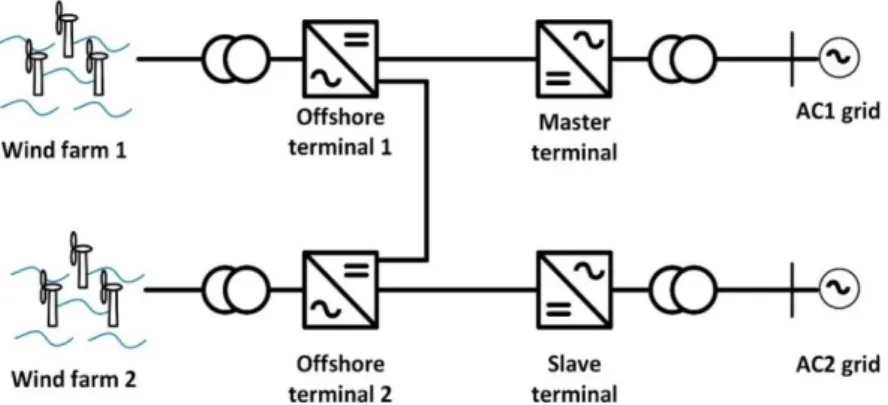
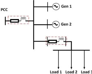
The MTDC network under study evacuates offshore wind energy to two onshore AC grids and is presented in Figure1. The MTDC network is composed by 2 onshore (master–slave) and 2 offshore VSC terminals. By means of HVDC links, each offshore VSC terminal is coupled to one onshore VSC terminal and both offshore terminals are coupled at the offshore side. Each HVDC link is made via bipolar HVDC cables with a length of 100 km and a rated voltage and current of 320 kV and 2373 kA, respectively. Each offshore VSC terminal is connected to an offshore wind farm composed by 100 wind turbines of 5.5 MVA each and with a 0.9 inductive-capacitive power factor range.
Energies 2020, 13, x FOR PEER REVIEW 4 of 21
The main requirements of the considered grid code in this paper have been described through this Section. However, there have been recent and minor modifications of this grid code, which can be consulted in [21].
3. Multi-Terminal Direct Current (MTDC) Grid Topology and Control Systems
The MTDC network under study evacuates offshore wind energy to two onshore AC grids and is presented in Figure 1. The MTDC network is composed by 2 onshore (master–slave) and 2 offshore VSC terminals. By means of HVDC links, each offshore VSC terminal is coupled to one onshore VSC terminal and both offshore terminals are coupled at the offshore side. Each HVDC link is made via bipolar HVDC cables with a length of 100 km and a rated voltage and current of 320 kV and 2373 kA, respectively. Each offshore VSC terminal is connected to an offshore wind farm composed by 100 wind turbines of 5.5 MVA each and with a 0.9 inductive-capacitive power factor range.
Figure 1. Multi-terminal direct current (MTDC) grid topology .
The HVDC links are also coupled to the onshore AC grid, whose maximum short circuit power is 30000 MVA and R/X ratio is 0.1.
Average models for onshore and offshore converters can be selected to simulate onshore faults with sufficient accuracy, since the present system is not equipped with fast offshore grid voltage reduction-based fault-ride-through function, as concluded in [22]. Therefore, a modular multilevel converter (MMC) average model is used to model the four terminals of the MTDC grid.
3.1. MTDC Grid Supervisory Control System
Before digging in details of the control systems at terminal level, an overview of the MTDC supervisory control system [7] is given. The MTDC supervisory control is responsible for the distribution of power references within the MTDC grid to convey wind energy from the offshore terminals into the onshore terminals in safe conditions. For this purpose, the role of the exchange mode is to set the DC power reference for the slave terminal, which is a function of the wind energy production coming from the two wind farms,
P
WF,1 andP
WF,2, by means of a proportional constantk
PRO, as Equation (1) shows.𝑃
, ,= 𝑘
(𝑃
,+ 𝑃
,) 0 𝑝. 𝑢. < 𝑃
, ,< 𝑃
, (1)Whenever there is a connection or disconnection event, the distribution of active power will be changed, and the slave terminal will increase or reduce its absorbed active power.
3.2. Control Systems at Terminal Level
At terminal level, the MTDC grid is composed, on the one hand, of two onshore terminals, i.e., the master and slave terminals, which are in charge of controlling the DC voltage and DC power,
Figure 1.Multi-terminal direct current (MTDC) grid topology.
The HVDC links are also coupled to the onshore AC grid, whose maximum short circuit power is 30,000 MVA and R/X ratio is 0.1.
Average models for onshore and offshore converters can be selected to simulate onshore faults with sufficient accuracy, since the present system is not equipped with fast offshore grid voltage reduction-based fault-ride-through function, as concluded in [22]. Therefore, a modular multilevel converter (MMC) average model is used to model the four terminals of the MTDC grid.
3.1. MTDC Grid Supervisory Control System
Before digging in details of the control systems at terminal level, an overview of the MTDC supervisory control system [7] is given. The MTDC supervisory control is responsible for the distribution of power references within the MTDC grid to convey wind energy from the offshore terminals into the onshore terminals in safe conditions. For this purpose, the role of the exchange mode is to set the DC power reference for the slave terminal, which is a function of the wind energy production coming from the two wind farms,PWF,1andPWF,2, by means of a proportional constant kPRO, as Equation (1) shows.
PDC,re f,slave = kPRO(PWF,1+PWF,2) 0p.u.<PDC,re f,slave<Pnom,slave (1)
Whenever there is a connection or disconnection event, the distribution of active power will be changed, and the slave terminal will increase or reduce its absorbed active power.
Energies2020,13, 2807 5 of 20
3.2. Control Systems at Terminal Level
At terminal level, the MTDC grid is composed, on the one hand, of two onshore terminals, i.e., the master and slave terminals, which are in charge of controlling the DC voltage and DC power, respectively. On the other hand, it is composed by two offshore terminals that convey the power produced by offshore wind farms.
3.2.1. Onshore Terminals
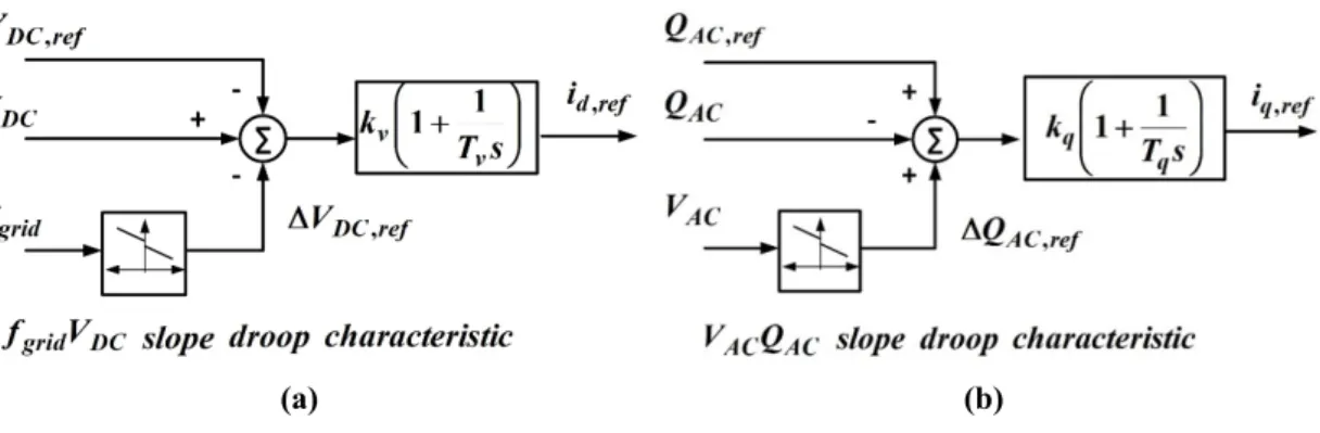
As mentioned previously, being the onshore master terminal responsible for controlling the DC voltage, it uses aVDCQscheme. By following this scheme, the DC voltage is controlled by means of id,ref(Figure2a) and includes afgridVDCslope characteristic where the LFSM/FSM frequency-response function is implemented by means of thekFSMparameter. Besides and according to theVDCQscheme, the reactive power is controlled by means ofiq,ref, where aVACQACslope droop function is included to
contribute to AC voltage stability of the AC grid (Figure2b).
Energies 2020, 13, x FOR PEER REVIEW 5 of 21
respectively. On the other hand, it is composed by two offshore terminals that convey the power produced by offshore wind farms.
3.2.1. Onshore Terminals
As mentioned previously, being the onshore master terminal responsible for controlling the DC voltage, it uses a
V
DCQ
scheme. By following this scheme, the DC voltage is controlled by means ofid,ref
(Figure 2a) and includes afgridVDC
slope characteristic where the LFSM/FSM frequency-response function is implemented by means of thek
FSM parameter. Besides and according to theV
DCQ
scheme,the reactive power is controlled by means of
i
q,ref, where aV
ACQ
AC slope droop function is includedto contribute to AC voltage stability of the AC grid (Figure 2b).
(a) (b)
Figure 2. Onshore master terminal control VDCQ scheme. Generation of: (a)
i
d,refand (b)i
q,ref.The onshore slave terminal oversees the active power and includes a
fgridPAC
characteristic where thek
FSM frequency-response function is implemented to comply with the frequency requirementsspecified in the UK national grid code, as in the master terminal. The slave terminal also contributes to DC voltage stability by means of a droop
VDCPAC
characteristic with dead band around the DC voltage reference. For this purpose, it follows aPQ
scheme where the control of reactive power is the same as in the onshore master terminal (Figure 2b). The difference with the master terminal is found at the generation of thei
d,ref, where active power magnitudes are operated instead of DC voltagevariables, as shown in Figure 3.
Figure 3. Onshore slave terminal with PQ scheme: generation of
id,ref
.The frequency-response functions in onshore master and slave terminals ensure the LFSM response and FSM modes already described in Section 2. The tuning parameters for achieving these
Figure 2.Onshore master terminal controlVDCQscheme. Generation of: (a)id,refand (b)iq,ref.
The onshore slave terminal oversees the active power and includes afgridPACcharacteristic where thekFSM frequency-response function is implemented to comply with the frequency requirements
specified in the UK national grid code, as in the master terminal. The slave terminal also contributes to DC voltage stability by means of a droopVDCPACcharacteristic with dead band around the DC voltage reference. For this purpose, it follows aPQscheme where the control of reactive power is the same as in the onshore master terminal (Figure2b). The difference with the master terminal is found at the generation of theid,ref, where active power magnitudes are operated instead of DC voltage variables, as shown in Figure3.
Energies 2020, 13, x FOR PEER REVIEW 5 of 21
respectively. On the other hand, it is composed by two offshore terminals that convey the power produced by offshore wind farms.
3.2.1. Onshore Terminals
As mentioned previously, being the onshore master terminal responsible for controlling the DC voltage, it uses a
VDCQ
scheme. By following this scheme, the DC voltage is controlled by means ofi
d,ref (Figure 2a) and includes af
gridV
DC slope characteristic where the LFSM/FSM frequency-responsefunction is implemented by means of the
k
FSM parameter. Besides and according to theV
DCQ
scheme,the reactive power is controlled by means of
iq,ref
, where aVACQAC
slope droop function is included to contribute to AC voltage stability of the AC grid (Figure 2b).(a) (b)
Figure 2. Onshore master terminal control VDCQ scheme. Generation of: (a)
id,ref
and (b)iq,ref
.The onshore slave terminal oversees the active power and includes a
f
gridP
ACcharacteristic wherethe
k
FSM frequency-response function is implemented to comply with the frequency requirementsspecified in the UK national grid code, as in the master terminal. The slave terminal also contributes to DC voltage stability by means of a droop
VDCPAC
characteristic with dead band around the DC voltage reference. For this purpose, it follows aPQ
scheme where the control of reactive power is the same as in the onshore master terminal (Figure 2b). The difference with the master terminal is found at the generation of theid,ref
, where active power magnitudes are operated instead of DC voltage variables, as shown in Figure 3.Figure 3. Onshore slave terminal with PQ scheme: generation of
i
d,ref.The frequency-response functions in onshore master and slave terminals ensure the LFSM response and FSM modes already described in Section 2. The tuning parameters for achieving these
Energies2020,13, 2807 6 of 20
The frequency-response functions in onshore master and slave terminals ensure the LFSM response and FSM modes already described in Section2. The tuning parameters for achieving these frequency droop loops are equal for both FSM and LFSM modes, thus implyingkFSM=kLFSM, and for the sake of simplicitykFSMis used from now on.
Furthermore, both master and slave terminals present the same inner proportional resonant control, already described in [7], and whose control parameters are detailed in AppendixA.
3.2.2. Offshore Terminals
The control scheme of the offshore terminals is depicted in Figure4. Each offshore terminal has a voltage controller in charge of regulating the amplitude and frequency of the AC voltage at each wind farm. This is done by means of a proportional integral (PI) controller, which obtains the modulation index required by the offshore converter, according to [7]. In order to limit the power generated by the whole farm during DC over-voltages due to contingencies, such as the loss of terminals or DC links, aVDCfgridcharacteristic is added, which allows to modify the wind farm grid frequency, taking advantage of the capability of the wind generators to change their generation against frequency variations.
Energies 2020, 13, x FOR PEER REVIEW 6 of 21
frequency droop loops are equal for both FSM and LFSM modes, thus implying
kFSM
=kLFSM
, and for the sake of simplicityk
FSMis used from now on.Furthermore, both master and slave terminals present the same inner proportional resonant control, already described in [7], and whose control parameters are detailed in Appendix.
3.2.2. Offshore Terminals
The control scheme of the offshore terminals is depicted in Figure 4.Each offshore terminal has a voltage controller in charge of regulating the amplitude and frequency of the AC voltage at each wind farm. This is done by means of a proportional integral (PI) controller, which obtains the modulation index required by the offshore converter, according to [7]. In order to limit the power generated by the whole farm during DC over-voltages due to contingencies, such as the loss of terminals or DC links, a
V
DCf
grid characteristic is added, which allows to modify the wind farm gridfrequency, taking advantage of the capability of the wind generators to change their generation against frequency variations.
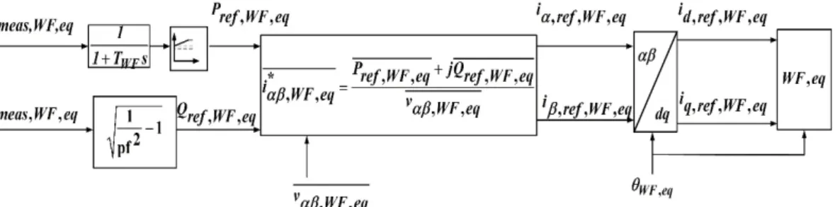
The control scheme for the offshore terminals is presented in [7], can also be complemented with the control of the offshore wind farm. The offshore wind farms in the present paper follows a control scheme presented in Figure 4, which corresponds to an equivalent wind farm model obtained by a simple aggregation technique. Therefore, the equivalent wind farm model consists in a single wind generator whose apparent power is the apparent power of a single wind generator multiplied by the number of wind generators of the wind farm.
Figure 4. Control schematic for the equivalent aggregated wind farm generator.
In Figure 4, the frequency and the active power of the aggregated wind farm model,
fmeas,WF,eq
and
P
meas,WF,eq, are measured to calculated the active and reactive power references of the aggregatedwind generator,
Pref,WF,eq
andQref,WF,eq
.The frequency measurement is first filtered by a first order delay, defined by
TWF
, which is aimed at attenuating oscillations provoked by the phase-locked loop (PLL).For frequency measurements, the PLL is adjusted to have an integral gain of 1 and a proportional gain of 10. Hereupon, the filtered frequency measurement is converted into active power magnitude by means of a
f-P
droop characteristic. This relates the offshore frequency variations with changes in the wind farm active power. The result of this operation turns to be the active power reference of the aggregated wind farm generator,P
ref,WF,eq.The active power at the output of the aggregated wind generator is measured to calculate the reactive power reference,
Qref,WF,eq
. Since the offshore wind farms follow a fixed power factor control, the reactive power reference is obtained from the measured active power and the chosen power factor.The current references in αβ frame,
i
α,ref,WF,eqandi
β,ref,WF,eq, are calculated by using the previouslycalculated,
Pref,WF,eq
andQref,WF,eq
magnitudes, jointly with the voltage vector, also in αβ frame, measured at the output of the aggregated wind farm generator,𝑣
𝛼𝛽,𝑊𝐹,𝑒𝑞. According to theFigure 4.Control schematic for the equivalent aggregated wind farm generator.
The control scheme for the offshore terminals is presented in [7], can also be complemented with the control of the offshore wind farm. The offshore wind farms in the present paper follows a control scheme presented in Figure4, which corresponds to an equivalent wind farm model obtained by a simple aggregation technique. Therefore, the equivalent wind farm model consists in a single wind generator whose apparent power is the apparent power of a single wind generator multiplied by the number of wind generators of the wind farm.
In Figure4, the frequency and the active power of the aggregated wind farm model,fmeas,WF,eqand
Pmeas,WF,eq, are measured to calculated the active and reactive power references of the aggregated wind
generator,Pref,WF,eqandQref,WF,eq.
The frequency measurement is first filtered by a first order delay, defined byTWF, which is aimed at attenuating oscillations provoked by the phase-locked loop (PLL).
For frequency measurements, the PLL is adjusted to have an integral gain of 1 and a proportional gain of 10. Hereupon, the filtered frequency measurement is converted into active power magnitude by means of af-Pdroop characteristic. This relates the offshore frequency variations with changes in the wind farm active power. The result of this operation turns to be the active power reference of the aggregated wind farm generator,Pref,WF,eq.
The active power at the output of the aggregated wind generator is measured to calculate the reactive power reference,Qref,WF,eq. Since the offshore wind farms follow a fixed power factor control, the reactive power reference is obtained from the measured active power and the chosen power factor. The current references inαβframe,iα,ref,WF,eqandiβ,ref,WF,eq, are calculated by using the previously
calculated,Pref,WF,eqandQref,WF,eqmagnitudes, jointly with the voltage vector, also inαβframe, measured at the output of the aggregated wind farm generator,vαβ,WF,eq. According to the operation shown in
Energies2020,13, 2807 7 of 20
Figure4, the current references in theαβframe are transformed into dq frame by means of the Park transform, considering the angle measured by the PLL,θWF,eq.
Finally, the aggregated wind farm generator is controlled by the dq current references,id,ref,WF,eq
andiq,ref,WF,eq, and theθWF,eqangle.
The aggregated wind-farm generator is modelled as a static generator and this implies that no dynamic functions of the wind turbines are included. This approach has been justified previously as adequate in the literature for the case of wind farms connected by means of an HVDC link [22], since the present study only deals with onshore faults. If offshore faults were considered, a more detailed wind turbine model would be necessary.
4. Open-Loop Frequency Response of the MTDC Grid
The control structure presented in Section3has been tested against the set of frequency steps recommended by the UK national grid code to validate the behaviour of the system under frequency excursions. This test is specified for testing the frequency response of power park modules and offshore transmission system user [19]. This test should be programmed when 95% of the power park units within a power park module is in service, according to [19], where the terms designed as power park units and module are properly defined. Furthermore, the simulated frequency deviations should be applied into the frequency controller reference summing junction, when the frequency controller is in FSM or LFSM mode [19]. In addition to this, the ability of the power park module to deliver a requested steady-state power output needs to be demonstrated [19].
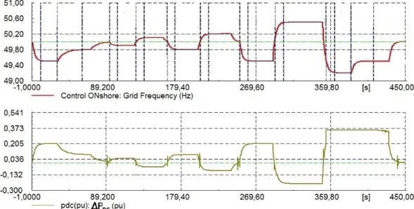
In Figure5, the frequency signal measured at the PCC and the power absorbed from the master terminal (∆PDC(p.u.)) are shown as a final proof of compliance with the frequency response. Different settling times have been obtained to reach set points of 10 s and 30 s as well as holding times of 20 s to maintain the frequency at a constant value at several stages of the sequence. The simulation results show that the proposed control structure is compliant with the grid code requirements.
Energies 2020, 13, x FOR PEER REVIEW 7 of 21
operation shown in Figure 4, the current references in the αβ frame are transformed into dq frame by means of the Park transform, considering the angle measured by the PLL,
θ
WF,eq.Finally, the aggregated wind farm generator is controlled by the dq current references,
id,ref,WF,eq
and
iq,ref,WF,eq
, and theθWF,eq
angle.The aggregated wind-farm generator is modelled as a static generator and this implies that no dynamic functions of the wind turbines are included. This approach has been justified previously as adequate in the literature for the case of wind farms connected by means of an HVDC link [22], since the present study only deals with onshore faults. If offshore faults were considered, a more detailed wind turbine model would be necessary.
4. Open-Loop Frequency Response of the MTDC Grid
The control structure presented in Section 3 has been tested against the set of frequency steps recommended by the UK national grid code to validate the behaviour of the system under frequency excursions. This test is specified for testing the frequency response of power park modules and offshore transmission system user [19]. This test should be programmed when 95% of the power park units within a power park module is in service, according to [19], where the terms designed as power park units and module are properly defined. Furthermore, the simulated frequency deviations should be applied into the frequency controller reference summing junction, when the frequency controller is in FSM or LFSM mode [19]. In addition to this, the ability of the power park module to deliver a requested steady-state power output needs to be demonstrated [19].
In Figure 5, the frequency signal measured at the PCC and the power absorbed from the master terminal (
Δ
P
DC (p.u.)) are shown as a final proof of compliance with the frequency response. Differentsettling times have been obtained to reach set points of 10 s and 30 s as well as holding times of 20 s to maintain the frequency at a constant value at several stages of the sequence. The simulation results show that the proposed control structure is compliant with the grid code requirements.
Figure 5. Response to frequency steps to UK grid code requirements.
In Figure 5, the green line corresponds to the level of 50 Hz and detailed information of the events can be consulted in [19].
5. Onshore Alternating Current (AC) Grid Model to Emulate Frequency Response
The test performed in Section 4 is an open-loop validation of the control against simulated frequency variations. In order to analyse the closed-loop response, additional validation tests are needed. In several countries, compliance with grid code requirements is allowed to be evaluated by
Figure 5.Response to frequency steps to UK grid code requirements.
In Figure5, the green line corresponds to the level of 50 Hz and detailed information of the events can be consulted in [19].
5. Onshore Alternating Current (AC) Grid Model to Emulate Frequency Response
The test performed in Section 4is an open-loop validation of the control against simulated frequency variations. In order to analyse the closed-loop response, additional validation tests are
Energies2020,13, 2807 8 of 20
needed. In several countries, compliance with grid code requirements is allowed to be evaluated by computer simulations, provided that the simulation models of the generating units are validated with real measurements during tests [1]. This happens, for example in Germany and Spain with the FGW-TG3 and the response of wind farms in the event of voltage dips (PVVC) procedure, respectively, according to [1]. For that purpose, in the literature frequency events have been introduced by random load increase or decrease events [15,16,23], random generation loss events for the study of under-frequency response [24,25], or by power system models such as the 3-bus great britain (GB) model and the simplified GB model in [26].
In the present paper, these disturbances will be introduced at the PCC of the onshore grid (AC1 in Figure6), replaced by an equivalent grid model parameterised for specific frequency events, with identical short-circuit power. The topology of this equivalent model is shown in Figure6.
Energies 2020, 13, x FOR PEER REVIEW 8 of 21
computer simulations, provided that the simulation models of the generating units are validated with real measurements during tests [1]. This happens, for example in Germany and Spain with the FGW-TG3 and the response of wind farms in the event of voltage dips (PVVC) procedure, respectively, according to [1]. For that purpose, in the literature frequency events have been introduced by random load increase or decrease events [15,16,23], random generation loss events for the study of under-frequency response [24,25], or by power system models such as the 3-bus great britain (GB) model and the simplified GB model in [26].
In the present paper, these disturbances will be introduced at the PCC of the onshore grid (AC1 in Figure 6), replaced by an equivalent grid model parameterised for specific frequency events, with identical short-circuit power. The topology of this equivalent model is shown in Figure 6.
Figure 6.Equivalent AC grid model for frequency event.
The PCC point shown in Figure 6 corresponds to the point of common coupling between the onshore master terminal and the AC1 grid corresponding to Figure 1.
The model is based on a SFR model, which represents an aggregate load-frequency behaviour following load-generation unbalance [27]. With the equivalent grid model, an under-frequency event can be emulated by the connection of an additional load (Load 3 in Figure 6) or the disconnection of a small generator (Gen 2 in in Figure 6). Therefore, a deficit in generation and excess of demand will be observed and an under-frequency event will occur. By contrast, an over-frequency event can be emulated by a partial load shedding (Load 2 in Figure 6, or by the connection of a small generator (Gen 2 in in Figure 6). This imposes an excess of generation and a deficit of demand, resulting in an over-frequency event. The inertia constant of the equivalent power system is represented by a single generating unit (generator Gen 1 in Figure 6), where a simplified first-order governor and excitation system models are used, based on [28]
Hence, several of the onshore grid model characteristic depend on the frequency event to emulate. Thus, a wide range of events can be simulated. By parameterising the equivalent model, frequency events can be simulated with specific frequency characteristics of rate-of-change-of-frequency (ROCOF), minimum/maximum frequency value (frequency nadir) and frequency deviation in steady-state. All three magnitudes can be calculated by using Equations (2), (3) and (4), respectively. The adjustment is based on an active power mismatch
Δ
P
0, which will be a generationtrip for under-frequency events and a load trip for over-frequency events.
In a power system with multiple generators, when part of the generation is lost, system frequency starts to drop. Assuming that all generators remain in synchronism, they slow down at approximately the same ROCOF as indicated in Equation (2).
∆𝑃 = 2
𝐻 𝑆
𝑆
𝑅𝑂𝐶𝑂𝐹 = 2𝐻 𝑅𝑂𝐶𝑂𝐹
(2)Figure 6.Equivalent AC grid model for frequency event.
The PCC point shown in Figure6corresponds to the point of common coupling between the onshore master terminal and the AC1 grid corresponding to Figure1.
The model is based on a SFR model, which represents an aggregate load-frequency behaviour following load-generation unbalance [27]. With the equivalent grid model, an under-frequency event can be emulated by the connection of an additional load (Load 3 in Figure6) or the disconnection of a small generator (Gen 2 in in Figure6). Therefore, a deficit in generation and excess of demand will be observed and an under-frequency event will occur. By contrast, an over-frequency event can be emulated by a partial load shedding (Load 2 in Figure6, or by the connection of a small generator (Gen 2 in in Figure6). This imposes an excess of generation and a deficit of demand, resulting in an over-frequency event. The inertia constant of the equivalent power system is represented by a single generating unit (generator Gen 1 in Figure6), where a simplified first-order governor and excitation system models are used, based on [28].
Hence, several of the onshore grid model characteristic depend on the frequency event to emulate. Thus, a wide range of events can be simulated. By parameterising the equivalent model, frequency events can be simulated with specific frequency characteristics of rate-of-change-of-frequency (ROCOF), minimum/maximum frequency value (frequency nadir) and frequency deviation in steady-state. All three magnitudes can be calculated by using Equations (2)–(4), respectively. The adjustment is based on an active power mismatch∆P0, which will be a generation trip for under-frequency events
Energies2020,13, 2807 9 of 20
In a power system with multiple generators, when part of the generation is lost, system frequency starts to drop. Assuming that all generators remain in synchronism, they slow down at approximately the sameROCOFas indicated in Equation (2).
∆P0 = 2 n X i=1 HiSi ST ROCOF = 2HeqROCOF (2)
In Equation (2),∆P0is the active power mismatch,Hi, andSithe inertia constant and the apparent
power of the individual generators making up the system,STthe total capacity in the system andHeq
the equivalent inertia of the system. The computation of frequency deviation in the steady-state value in a power system with several generators is also straightforward by applying Equation (3).
∆P0 = n X i=1 1 Rdroop,i +Dt ∆fss = 1 Rdroop,eq +Dt ! ∆fss (3)
In Equation (3),Rdroop,iis the droop constant of the individual generators making up the system,
Dt, the damping constant in the system, andRdroop,eqthe equivalent droop constant in the system.
The calculation of the minimum frequency after an active power mismatch depends on the frequency-response strategies of the network assets, such as conventional generating units, renewable generating units, storage systems or demand assets. Therefore, the equivalent SFR model results in a complex function dependent on several variables. Consequently, several authors have introduced simplifying hypotheses in order to compute frequency response in a power system [22,23].
In the present case, the equivalent power system is represented by a single generating unit with a simplified first-order governor and excitation system model. Therefore, the adjustment for the frequency minimum/maximum value results in Equation (4):
∆P0 = ∆fmin
Dt+Keq
1+e−√ςωntmin
1−ς2
Teqωnsin(ωrtmin)−sin(ωrtmin+θ1)
(4)
In Equation (4),ωr,ωn,ζ, andθ1can be calculated based on [16] and considering a first-order
system.KeqandTeqare respectively the gain and time constant of the first-order governor in Gen 1 and
tminis calculated with Equation (5):
tmin =
1
ωratan
ωnTeqp1−ς2
ωnTeqς−1 (5)
The values of the control parameters for the onshore AC grid model are summarised in AppendixA. 6. Novel Methodology to Tune MTDC Supervisory and Frequency-Response Control Functions at Terminal Level in Over-Frequency Events
In this section the novelty of the present paper is described, i.e., the methodology to tune jointly the supervisory and frequency-response control functions of outer loops at terminal level. In Figure7, the complete system of the MTDC grid connected to the onshore AC grid model is depicted. This contains the MTDC grid, described in Section3, connected to the onshore AC grid model to simulate the frequency events applied at the PCC point shown in Figure7.
Energies2020,13, 2807 10 of 20
Energies 2020, 13, x FOR PEER REVIEW 10 of 21
Figure 7. Closed-loop MTDC system connected to the considered equivalent onshore AC grid model.
In Figure 8, a flowchart of the methodology, applied to the system in Figure 7, is exposed, where the supervisory control and the frequency-response functions of the onshore terminals are two major aspects to define the tuning strategies in order to obtain reductions in the frequency peak. Besides, for certain levels of
kFSM
value, even the order type of the frequency signal may be reduced from 2nd order to 1st order.Therefore, the flowchart in Figure 8 allows two control levels of the hierarchical MTDC coordinated control structure to be tuned simultaneously.
On the one hand, it allows the MTDC supervisory control to be tuned, by means of choosing the proper active power exchange set point (from now on,
PDC,ref,slave
). The values tested forPDC,ref,slave
have been selected according to four equal shares of the maximum capacity of the slave terminal.On the other hand, it allows the outer loop control of onshore terminals to be parameterised by means of setting the proper slope for the frequency response (
kFSM
). The values thatkFSM
adopts are chosen among those recommended by the UK national grid code [19,20] (3%–5%), and even trying greater values such as 7.5% to check for further improvements.Figure 7.Closed-loop MTDC system connected to the considered equivalent onshore AC grid model. In Figure8, a flowchart of the methodology, applied to the system in Figure7, is exposed, where the supervisory control and the frequency-response functions of the onshore terminals are two major aspects to define the tuning strategies in order to obtain reductions in the frequency peak. Besides, for certain levels ofkFSMvalue, even the order type of the frequency signal may be reduced from 2nd
order to 1st order.Energies 2020, 13, x FOR PEER REVIEW 11 of 21
Figure 8. Diagram of novel methodology to design MTDC master and slave terminal outer loop control.
The definition of tuning strategies is detailed in Table 1, where the values for both
P
DC,ref,slave andk
FSM are clarified.Table 1. Definition of tuning strategies according to kFSM and PDC,ref,slave. Strategies kFSM PDC,ref,slave
Strategy 1 0%
0.25 0.5 0.75 1 Strategy 2 5%
Strategy 3 7.5%
These tuning strategies are aimed at reducing the frequency peak at the PCC of the onshore AC grid. Indeed, the proper combination of both
P
DC,ref,slave or thek
FSM values can also transform the 2ndorder nature of the frequency excursion into a 1st order nature.
Furthermore, the sensitivity of the tuning strategies must be checked against variations in the parameters of the synchronous generator, such as the equivalent inertia or damping. According to this sensitivity analysis, the peak of frequency will also experience changes and therefore, the optimal strategy may vary.
If the frequency peak is not sufficiently smoothed by a strategy for a specific case, then
P
DC,ref,slaveor the
k
FSM values can be readjusted and reductions of the frequency peak at PCC can be checked.For this purpose, a threshold value for frequency can be selected and the established limit for the LFSM band, i.e., 50.4 Hz, is proposed. In this way, this limit bounds the frequency signal out of the LFSM compulsory band, and therefore, the risk of instability is reduced.
Figure 8.Diagram of novel methodology to design MTDC master and slave terminal outer loop control. Therefore, the flowchart in Figure8allows two control levels of the hierarchical MTDC coordinated control structure to be tuned simultaneously.
Energies2020,13, 2807 11 of 20
On the one hand, it allows the MTDC supervisory control to be tuned, by means of choosing the proper active power exchange set point (from now on,PDC,ref,slave). The values tested forPDC,ref,slave
have been selected according to four equal shares of the maximum capacity of the slave terminal. On the other hand, it allows the outer loop control of onshore terminals to be parameterised by means of setting the proper slope for the frequency response (kFSM). The values thatkFSM adopts are chosen among those recommended by the UK national grid code [19,20] (3–5%), and even trying greater values such as 7.5% to check for further improvements.
The definition of tuning strategies is detailed in Table1, where the values for bothPDC,ref,slaveand
kFSMare clarified.
Table 1.Definition of tuning strategies according tokFSMandPDC,ref,slave. Strategies kFSM PDC,ref,slave
Strategy 1 0%
0.25 0.5 0.75 1
Strategy 2 5%
Strategy 3 7.5%
These tuning strategies are aimed at reducing the frequency peak at the PCC of the onshore AC grid. Indeed, the proper combination of bothPDC,ref,slaveor thekFSMvalues can also transform the 2nd order nature of the frequency excursion into a 1st order nature.
Furthermore, the sensitivity of the tuning strategies must be checked against variations in the parameters of the synchronous generator, such as the equivalent inertia or damping. According to this sensitivity analysis, the peak of frequency will also experience changes and therefore, the optimal strategy may vary.
If the frequency peak is not sufficiently smoothed by a strategy for a specific case, thenPDC,ref,slave
or thekFSMvalues can be readjusted and reductions of the frequency peak at PCC can be checked. For this purpose, a threshold value for frequency can be selected and the established limit for the LFSM band, i.e., 50.4 Hz, is proposed. In this way, this limit bounds the frequency signal out of the LFSM compulsory band, and therefore, the risk of instability is reduced.
Each of the strategies can be ranked upon the reduction of maximum frequency peak they can achieve. Therefore, most of the novelty of the proposed methodology is based on the implication of different control levels jointly for proper tuning of the control structure and the verification of the improvements by means of maximum frequency peak reductions.
7. Application Case of the Methodology to the Considered MTDC+Onshore AC Grid
The methodology proposed in the present paper is applied to a case study consisting in the system presented in Figure7, by means of electro-magnetic transient (EMT) simulations carried out in DIgSILENT PF software. (Version 2019 SP3 (x64), DIgSILENT GmbH, Gomaringen, Germany) This system is tested under constant wind energy production, where each wind farm produces 400 MW. For this purpose, the coordinated control structure is tested against frequency excursions using the AC grid equivalent model introduced in Section5. The control parameters selected for both MTDC and onshore AC grid are detailed in AppendixA. A short-circuit ratio of 20.5 measured at the PCC has been considered. The analysed system consists of two loads of 890.5 MW and 250 MW, Load 1 and Load 2 respectively, as shown in Figure7. When the 250 MW load is disconnected, an over-frequency deviation (>50.4 Hz) is observed at the PCC, making the system work under the LFSM frequency band. The system enters the over-frequency FSM band by disconnecting Load 2 in Figure7. In this case, 120 MW is the load value considered to disconnect, since the provoked frequency excursions are within FSM bonds, i.e., lower than 50.5 Hz and higher than 50.015 Hz in case of over-frequency.
Energies2020,13, 2807 12 of 20
7.1. Impact of Tuning Strategies on the Reduction of the Frequency Peak
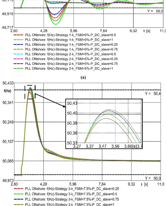
The benefit of implementing a frequency response at onshore terminal level, i.e., the reduction of transient frequency oscillation amplitude, is shown Figure9a,b, by means of the implementation of diEnergies fferent tuning strategies according to Table2020, 13, x FOR PEER REVIEW 1. 13 of 21
Figure 9. Frequency peak values for different strategies (
kFSM
) andPDC,ref,slave
values: (a) strategies 1 and 2 and (b) strategy 3.In Figure 10, the reductions in frequency peak among strategies are compared by taking into account the
PDC,ref,slave
values. The greatest improvements in frequency peak are observed for strategy 3 withk
FSM = 7.5% andP
DC,ref,slave= 0.25, reaching 50.39 Hz , and the worst case is observed for strategy1 with
P
DC,ref,slave= 1, reaching 50.66 Hz, as seen in Figure 10. (a)(b)
Figure 9.Frequency peak values for different strategies (kFSM) andPDC,ref,slavevalues: (a) strategies 1
Energies2020,13, 2807 13 of 20
In Figure9a, the reduction of the frequency peak value when a frequency-response function is implemented, namelykFSM=5% (strategy 2) can be observed with respect to the original system without
frequency-response function, i.e.,kFSM=0% (strategy 1). Both tuning strategies are parameterised according to differentPDC,ref,slavevalues, in order to further reduce the peak value in a more moderate manner than with the change ofkFSM, so that the lowestPDC,ref,slavevalue yields to the greatest peak frequency reduction.
Furthermore, in Figure9a, the inclusion of the frequency-response function not only reduces the frequency peak, but also changes the frequency curve order from second-order type withkFSM=0% to first-order type withkFSM =5%. An intermediate value ofkFSM =3% has been also simulated
and this presents a second-order type, but for the sake of clarity it has been removed from Figure9a. ThekFSM=5% is the limit value up to which the frequency curve is a second-order type. For larger values, such askFSM=7.5%, the first order type curve is still maintained and further greater reductions in the frequency peak are shown, as depicted in Figure9b.
Therefore, bothPDC,ref,slaveandkFSMvariables contribute to this peak reduction slightly and more
considerably, respectively, beingkFSM even capable of changing the polynomial order type of the frequency signal andPDC,ref,slave values able to slightly modify the final peak value derived from
kFSMvariation.
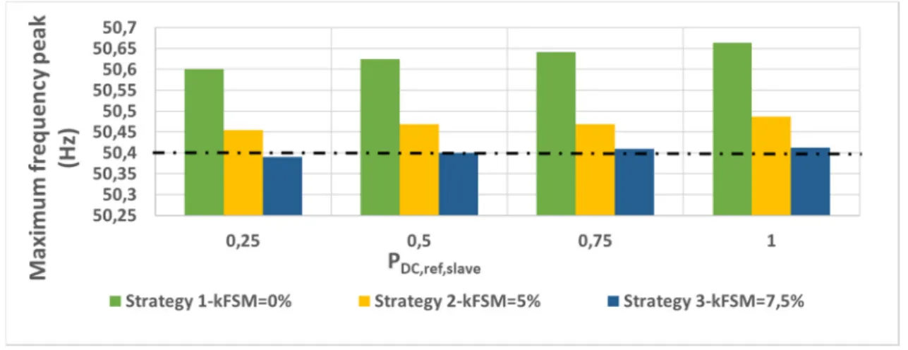
In Figure10, the reductions in frequency peak among strategies are compared by taking into account thePDC,ref,slavevalues. The greatest improvements in frequency peak are observed for strategy 3 withkFSM=7.5% andPDC,ref,slave=0.25, reaching 50.39 Hz, and the worst case is observed for strategy 1 withPDC,ref,slave=1, reaching 50.66 Hz, as seen in Figure10.
Energies 2020, 13, x FOR PEER REVIEW 14 of 21
Figure 10. Comparison of frequency peak values among curves in Figure 9.
If the strategies are compared within the same
k
FSM value, one can distinguish that for 0, 5 and7.5%, the greatest
PDC,ref,slave
value leads to the largest frequency peak value. Therefore, those strategies which employ highPDC,ref,slave
set points lead to worst case scenarios for a givenkFSM
. This can be especially observed in frequency peak reduction provided by strategy 1, which presents the greatest improvements made byP
DC,ref,slavevalues from all the selected cases, as the target variablesare reduced more drastically when
PDC,ref,slave
is decreased from 1 to 0.25.If the strategies are compared within the same
PDC,ref,slave
set point value, greater reductions in frequency peaks are obtained as far ask
FSM is increased. Moreover, severalP
DC,ref,slavevalues achievein strategy 3 frequency peak values lower than 50.4 Hz, namely,
PDC,ref,slave
= 0.25 andPDC,ref,slave
= 0.5. These combinations ensure that the complete frequency signal is out of the LFSM compulsory zone, where mandatory extra frequency response should be added if frequency values greater than 50.4 Hz are maintained.The benefits of having implemented the combined effects of both kFSMand
PDC,ref,slave
valuescorrespond to a case where an optional FSM ancillary service would be contracted. When the frequency-response function is contracted with the electrical utility as an ancillary service, several considerations must be addressed. In [29], a typical frequency response for a synchronous area under frequency disturbances for effective primary control is shown. In [29], the response is exemplified with an under-frequency event where the transient behaviour is characterised by oscillations and a time response from 15 s to 30 s. Therefore, it is important to test these reductions for a certain variation of the synchronous generator parameters. Among tuning strategies, strategy 2 (
k
FSM = 5%) is chosendue to its intermediate reduction of the frequency peak and being
kFSM
= 5% a limit value for the first-order behaviour of the frequency curve at PCC.7.2. Guidance for Tuning
k
FSM andP
DC,ref,slavewhen Different MTDC Control Structure and Synchronous Generator Characteristics Are ConsideredIn this Section, the frequency peak reduction is analysed within a specific strategy chosen from the previous analysis conducted in Section 7.1. The main objective of this Section is to give systematic guidance for adjusting the two control-level parameters,
k
FSMandP
DC,ref,slave, when the controlstructure of the MTDC grid is varied, i.e. instead of master–slave, a distributed control scheme, or the onshore AC grid characteristics are modified.
Strategy 2, while encompassing the whole range of
PDC,ref,slave
, implies a moderate tuning of the frequency-response function,k
FSM = 5%, of onshore terminals.According to CC.6.3.7(c)(ii) in [19,20], the
k
FSM for the LFSM mode has to be at least 2% per each0.1 Hz. In principle, for those frequency ranges that belong to the LFSM band there would be no
Figure 10.Comparison of frequency peak values among curves in Figure9.
If the strategies are compared within the samekFSMvalue, one can distinguish that for 0, 5 and
7.5%, the greatestPDC,ref,slavevalue leads to the largest frequency peak value. Therefore, those strategies
which employ highPDC,ref,slaveset points lead to worst case scenarios for a givenkFSM. This can be especially observed in frequency peak reduction provided by strategy 1, which presents the greatest improvements made byPDC,ref,slavevalues from all the selected cases, as the target variables are reduced
more drastically whenPDC,ref,slaveis decreased from 1 to 0.25.
If the strategies are compared within the samePDC,ref,slaveset point value, greater reductions in frequency peaks are obtained as far askFSMis increased. Moreover, severalPDC,ref,slavevalues achieve in strategy 3 frequency peak values lower than 50.4 Hz, namely,PDC,ref,slave=0.25 andPDC,ref,slave=0.5.
These combinations ensure that the complete frequency signal is out of the LFSM compulsory zone, where mandatory extra frequency response should be added if frequency values greater than 50.4 Hz are maintained.
Energies2020,13, 2807 14 of 20
The benefits of having implemented the combined effects of bothkFSMandPDC,ref,slavevalues correspond to a case where an optional FSM ancillary service would be contracted. When the frequency-response function is contracted with the electrical utility as an ancillary service, several considerations must be addressed. In [29], a typical frequency response for a synchronous area under frequency disturbances for effective primary control is shown. In [29], the response is exemplified with an under-frequency event where the transient behaviour is characterised by oscillations and a time response from 15 s to 30 s. Therefore, it is important to test these reductions for a certain variation of the synchronous generator parameters. Among tuning strategies, strategy 2 (kFSM=5%) is chosen due to its intermediate reduction of the frequency peak and beingkFSM=5% a limit value for the
first-order behaviour of the frequency curve at PCC.
7.2. Guidance for Tuning kFSMand PDC,ref,slavewhen Different MTDC Control Structure and Synchronous Generator Characteristics Are Considered
In this Section, the frequency peak reduction is analysed within a specific strategy chosen from the previous analysis conducted in Section7.1. The main objective of this Section is to give systematic guidance for adjusting the two control-level parameters,kFSMandPDC,ref,slave, when the control structure
of the MTDC grid is varied, i.e., instead of master–slave, a distributed control scheme, or the onshore AC grid characteristics are modified.
Strategy 2, while encompassing the whole range ofPDC,ref,slave, implies a moderate tuning of the frequency-response function,kFSM=5%, of onshore terminals.
According to CC.6.3.7(c)(ii) in [19,20], thekFSM for the LFSM mode has to be at least 2% per each 0.1 Hz. In principle, for those frequency ranges that belong to the LFSM band there would be no problem since,kFSM =7.5% exceeds this recommended minimum slope of 2% per each 0.1 Hz.
However, for those frequency values belonging to the FSM band, the recommendedkFSMvalue lays
between 3% and 5% per each 0.1 Hz, as reported in [20]. By contrast, these boundaries forkFSMwithin the FSM band are neither justified in the grid code [19] nor in the guidance note for DC converter stations [20].
To the best knowledge of the authors,kFSM=7.5% could imply a bit aggressive control, considering
that the FSM frequency range is narrower than the LFSM range. Moreover, although not considered in this paper,kFSMcan also present an opposite sign, as it should also consider under-frequency values with respect to 50 Hz. However, this could be more critical for a more complex distributed frequency control structure with a specifically located centre of inertia; nevertheless, the present paper considers a hierarchical master–slave structure. Therefore, more moderate values ofkFSMare recommended for distributed control structures than in master–slave structures, whilePDC,ref,slavecan be varied for the entire range, as it conducts to lower peak reductions or just peak amendment.
As for the onshore AC grid characteristics, several parameters of the main synchronous generator of the onshore AC grid are varied to extract guidelines on how to tune jointly the MTDC supervisory and outer loop frequency-response functions. According to the previous discussion, a moderatekFSM
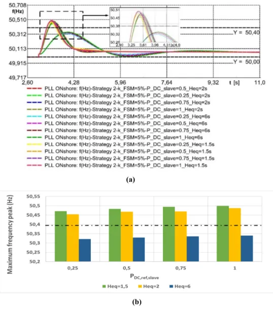
value is recommended and thus strategy 2 of Table1has been chosen. Therefore, strategy 2 is selected to be evaluated against a variation of the Gen 1 synchronous generator characteristics, such as the total inertia,Heq, and the damping,Dt, according to Equations (2)–(4). Strategy 2 is tested against a variation ofHeq, adopting the values of 1.5 s, 2 s and 6 s, and the impact on the frequency peak is shown in Figure11a.
In Figure11a, theHeq=6 s conducts to the slowest set of curves as well as the greatest reductions (50.32 Hz withPDC,ref,slave=0.25), whileHeq=1.5 s conducts to the fastest profiles and smaller reductions of the peak (50.49 Hz withPDC,ref,slave=1).
According to Figure11b thePDC,ref,slavevalues also contribute to the decrease of the peak values,
as far as they are reduced. TheHeq=6 s value yields to frequency values out of the compulsory LFSM zone since the peak values are lower than 50.4 Hz. This strategy would ensure that the complete
Energies2020,13, 2807 15 of 20
frequency signal is out of the LFSM compulsory zone, where mandatory extra frequency response should be added if frequency values greater than 50.4 Hz are maintained.
Energies 2020, 13, x FOR PEER REVIEW 15 of 21
problem since,
k
FSM = 7.5% exceeds this recommended minimum slope of 2% per each 0.1 Hz.However, for those frequency values belonging to the FSM band, the recommended
kFSM
value lays between 3% and 5% per each 0.1 Hz, as reported in[20]. By contrast, these boundaries forkFSM
within the FSM band are neither justified in the grid code [19] nor in the guidance note for DC converter stations [20].To the best knowledge of the authors,
kFSM
= 7.5% could imply a bit aggressive control, considering that the FSM frequency range is narrower than the LFSM range. Moreover, although not considered in this paper,k
FSM can also present an opposite sign, as it should also considerunder-frequency values with respect to 50Hz. However, this could be more critical for a more complex distributed frequency control structure with a specifically located centre of inertia; nevertheless, the present paper considers a hierarchical master–slave structure. Therefore, more moderate values of
k
FSM are recommended for distributed control structures than in master–slave structures, whileP
DC,ref,slavecan be varied for the entire range, as it conducts to lower peak reductions or just peakamendment.
As for the onshore AC grid characteristics, several parameters of the main synchronous generator of the onshore AC grid are varied to extract guidelines on how to tune jointly the MTDC supervisory and outer loop frequency-response functions. According to the previous discussion, a moderate
kFSM
value is recommended and thus strategy 2 of Table 1 has been chosen. Therefore, strategy 2 is selected to be evaluated against a variation of the Gen 1 synchronous generator characteristics, such as the total inertia,H
eq, and the damping,D
t, according to Equations (2)–(4).Strategy 2 is tested against a variation of
H
eq, adopting the values of 1.5 s, 2 s and 6 s, and the impacton the frequency peak is shown in Figure 11a.
(a)
Energies 2020, 13, x FOR PEER REVIEW 16 of 21
Figure 11. Sensitivity analysis for the variation of
Heq
: (a)frequency curves for strategy 2 for differentP
DC,ref,slaveset points and Heq values and (b) comparison of frequency peak values among curves in (a).In Figure 11a, the Heq = 6 s conducts to the slowest set of curves as well as the greatest reductions
(50.32 Hz with PDC,ref,slave = 0.25), while Heq = 1.5 s conducts to the fastest profiles and smaller reductions
of the peak (50.49 Hz with PDC,ref,slave=1).
According to Figure 11b the PDC,ref,slavevalues also contribute to the decrease of the peak values,
as far as they are reduced. The Heq = 6 s value yields to frequency values out of the compulsory LFSM
zone since the peak values are lower than 50.4 Hz. This strategy would ensure that the complete frequency signal is out of the LFSM compulsory zone, where mandatory extra frequency response should be added if frequency values greater than 50.4 Hz are maintained.
Therefore, for Heqvalues close to 6 s, it may be sufficient to tune PDC,ref,slavevalues to smooth the
peak and ensure the frequency signal outside the LFSM range. In contrast, for Heqvalues close to 1.5–
2 s, the curves are transiently inside of the LFSM zone, but getting out of this area thanks to the frequency-response function. Therefore, for large Heq values, a smaller kFSM value than 5% could also
provoke reductions in the peak, while PDC,ref, slave is kept to a minimum. For lower Heq values, a
substantially greater kFSM value would be needed, in order to achieve greater peak reductions.
As for the sensitivity against the variation of
D
t, the complete model has been tested whenD
tadopts the values of 0, 1.25 and 2.5, which would lead to a system without and with damping, respectively. In Figure 12a, the effect of these variations on the frequency behaviour is shown, and in Figure 12b, the peak values are compared.
In Figure 12a, two sets of curves are derived, one corresponding to
D
t = 0, with the greatest peakvalues, and another with
D
t = 2.5, leading to peak reductions. Apart from this, the decrease of thePDC,ref,slave
values contribute to the peak reduction. WithDt
= 2.5, the frequency peak is outside the LFSM compulsory area when thePDC,ref,slave
value equals to 0.25.Therefore, for a null
D
t value, a greaterk
FSM value than 5% has a great influence in achievingpeak reductions in a more efficient way than
P
DC,ref, slave. However, for greaterD
t values, just bymaintaining a low
PDC,ref, slave
value, the peak reduction is easily obtained, without the need for increasing thek
FSM slope.(b)
Figure 11.Sensitivity analysis for the variation ofHeq: (a) frequency curves for strategy 2 for different PDC,ref,slaveset points andHeqvalues and (b) comparison of frequency peak values among curves in (a).
Therefore, forHeqvalues close to 6 s, it may be sufficient to tunePDC,ref,slavevalues to smooth the peak and ensure the frequency signal outside the LFSM range. In contrast, forHeqvalues close to 1.5–2 s, the curves are transiently inside of the LFSM zone, but getting out of this area thanks to the frequency-response function. Therefore, for largeHeqvalues, a smallerkFSMvalue than 5% could
also provoke reductions in the peak, whilePDC,ref, slaveis kept to a minimum. For lowerHeqvalues, a substantially greaterkFSMvalue would be needed, in order to achieve greater peak reductions.
As for the sensitivity against the variation ofDt, the complete model has been tested when
Dtadopts the values of 0, 1.25 and 2.5, which would lead to a system without and with damping, respectively. In Figure12a, the effect of these variations on the frequency behaviour is shown, and in Figure12b, the peak values are compared.