Chapter 1
The Riemann Integral
I know of some universities in England where the Lebesgue integral is taught in the first year of a mathematics degree instead of the Riemann integral, but I know of no universities in England where students learn the Lebesgue integral in the first year of a mathematics degree. (Ap-proximate quotation attributed to T. W. K¨orner)
Let f : [a, b] → R be a bounded (not necessarily continuous) function on a compact (closed, bounded) interval. We will define what it means for f to be Riemann integrable on [a, b] and, in that case, define its Riemann integral Rb
a f.
The integral off on [a, b] is a real number whose geometrical interpretation is the signed area under the graph y =f(x) fora ≤x≤b. This number is also called the definite integral off. By integratingf over an interval [a, x] with varying right end-point, we get a function ofx, called the indefinite integral off.
The most important result about integration is the fundamental theorem of calculus, which states that integration and differentiation are inverse operations in an appropriately understood sense. Among other things, this connection enables us to compute many integrals explicitly.
Integrability is a less restrictive condition on a function than differentiabil-ity. Roughly speaking, integration makes functions smoother, while differentiation makes functions rougher. For example, the indefinite integral of every continuous function exists and is differentiable, whereas the derivative of a continuous function need not exist (and generally doesn’t).
The Riemann integral is the simplest integral to define, and it allows one to integrate every continuous function as well as some not-too-badly discontinuous functions. There are, however, many other types of integrals, the most important of which is the Lebesgue integral. The Lebesgue integral allows one to integrate unbounded or highly discontinuous functions whose Riemann integrals do not exist, and it has better mathematical properties than the Riemann integral. The defini-tion of the Lebesgue integral requires the use of measure theory, which we will not 1
describe here. In any event, the Riemann integral is adequate for many purposes, and even if one needs the Lebesgue integral, it’s better to understand the Riemann integral first.
1.1. Definition of the Riemann integral
We say that two intervals are almost disjoint if they are disjoint or intersect only at a common endpoint. For example, the intervals [0,1] and [1,3] are almost disjoint, whereas the intervals [0,2] and [1,3] are not.
Definition 1.1. LetIbe a nonempty, compact interval. A partition ofIis a finite collection{I1, I2, . . . , In}of almost disjoint, nonempty, compact subintervals whose
union is I.
A partition of [a, b] with subintervals Ik = [xk−1, xk] is determined by the set
of endpoints of the intervals
a=x0< x1< x2<· · ·< xn−1< xn =b.
Abusing notation, we will denote a partitionP either by its intervals P ={I1, I2, . . . , In}
or by the set of endpoints of the intervals
P ={x0, x1, x2, . . . , xn−1, xn}.
We’ll adopt either notation as convenient; the context should make it clear which one is being used. There is always one more endpoint than interval.
Example 1.2. The set of intervals
{[0,1/5],[1/5,1/4],[1/4,1/3],[1/3,1/2],[1/2,1]}
is a partition of [0,1]. The corresponding set of endpoints is
{0,1/5,1/4,1/3,1/2,1}. We denote the length of an intervalI= [a, b] by
|I|=b−a.
Note that the sum of the lengths|Ik|=xk−xk−1of the almost disjoint subintervals in a partition{I1, I2, . . . , In}of an intervalIis equal to length of the whole interval.
This is obvious geometrically; algebraically, it follows from the telescoping series
n X k=1 |Ik|= n X k=1 (xk−xk−1) =xn−xn−1+xn−1−xn−2+· · ·+x2−x1+x1−x0 =xn−x0 =|I|.
Suppose that f : [a, b] → R is a bounded function on the compact interval I= [a, b] with
M = sup
I
f, m= inf
1.1. Definition of the Riemann integral 3
IfP ={I1, I2, . . . , In} is a partition ofI, let
Mk = sup Ik
f, mk = inf Ik
f.
These suprema and infima are well-defined, finite real numbers sincef is bounded. Moreover,
m≤mk≤Mk≤M.
If f is continuous on the intervalI, then it is bounded and attains its maximum and minimum values on each subinterval, but a bounded discontinuous function need not attain its supremum or infimum.
We define the upper Riemann sum off with respect to the partitionP by U(f;P) = n X k=1 Mk|Ik|= n X k=1 Mk(xk−xk−1),
and the lower Riemann sum off with respect to the partitionP by L(f;P) = n X k=1 mk|Ik|= n X k=1 mk(xk−xk−1).
Geometrically,U(f;P) is the sum of the areas of rectangles based on the intervals Ik that lie above the graph off, andL(f;P) is the sum of the areas of rectangles
that lie below the graph off. Note that
m(b−a)≤L(f;P)≤U(f;P)≤M(b−a).
Let Π(a, b), or Π for short, denote the collection of all partitions of [a, b]. We define the upper Riemann integral of f on [a, b] by
U(f) = inf
P∈ΠU(f;P).
The set {U(f;P) : P ∈ Π} of all upper Riemann sums of f is bounded from below by m(b−a), so this infimum is well-defined and finite. Similarly, the set
{L(f;P) :P ∈Π}of all lower Riemann sums is bounded from above by M(b−a), and we define the lower Riemann integral off on [a, b] by
L(f) = sup
P∈Π
L(f;P).
These upper and lower sums and integrals depend on the interval [a, b] as well as the functionf, but to simplify the notation we won’t show this explicitly. A commonly used alternative notation for the upper and lower integrals is
U(f) = Z b a f, L(f) = Z b a f.
Note the use of “lower-upper” and “upper-lower” approximations for the inte-grals: we take the infimum of the upper sums and the supremum of the lower sums. As we show in Proposition 1.13 below, we always haveL(f)≤U(f), but in general the upper and lower integrals need not be equal. We define Riemann integrability by their equality.
Definition 1.3. A bounded functionf : [a, b]→Ris Riemann integrable on [a, b] if its upper integral U(f) and lower integral L(f) are equal. In that case, the Riemann integral off on [a, b], denoted by
Z b a f(x)dx, Z b a f, Z [a,b] f or similar notations, is the common value ofU(f) andL(f).
An unbounded function is not Riemann integrable. In the following, “grable” will mean “Riemann integrable, and “integral” will mean “Riemann inte-gral” unless stated explicitly otherwise.
1.2. Examples of the Riemann integral
Let us illustrate the definition of Riemann integrability with a number of examples. Example 1.4. Definef : [0,1]→Rby f(x) = ( 1/x if 0< x≤1, 0 ifx= 0. Then Z 1 0 1 xdx
isn’t defined as a Riemann integral becuasef is unbounded. In fact, if 0< x1< x2<· · ·< xn−1<1
is a partition of [0,1], then
sup [0,x1]
f =∞, so the upper Riemann sums off are not well-defined.
An integral with an unbounded interval of integration, such as
Z ∞
1 1 xdx,
also isn’t defined as a Riemann integral. In this case, a partition of [1,∞) into finitely many intervals contains at least one unbounded interval, so the correspond-ing Riemann sum is not well-defined. A partition of [1,∞) into bounded intervals (for example,Ik = [k, k+ 1] withk∈N) gives an infinite series rather than a finite
Riemann sum, leading to questions of convergence.
One can interpret the integrals in this example as limits of Riemann integrals, or improper Riemann integrals,
Z 1 0 1 xdx= limǫ→0+ Z 1 ǫ 1 xdx, Z ∞ 1 1 xdx= limr→∞ Z r 1 1 xdx,
but these are not proper Riemann integrals in the sense of Definition 1.3. Such improper Riemann integrals involve two limits — a limit of Riemann sums to de-fine the Riemann integrals, followed by a limit of Riemann integrals. Both of the improper integrals in this example diverge to infinity. (See Section 1.10.)
1.2. Examples of the Riemann integral 5
Next, we consider some examples of bounded functions on compact intervals. Example 1.5. The constant functionf(x) = 1 on [0,1] is Riemann integrable, and
Z 1
0
1dx= 1.
To show this, letP ={I1, I2, . . . , In} be any partition of [0,1] with endpoints {0, x1, x2, . . . , xn−1,1}. Sincef is constant, Mk = sup Ik f = 1, mk = inf Ik f = 1 fork= 1, . . . , n, and therefore U(f;P) =L(f;P) = n X k=1 (xk−xk−1) =xn−x0= 1.
Geometrically, this equation is the obvious fact that the sum of the areas of the rectangles over (or, equivalently, under) the graph of a constant function is exactly equal to the area under the graph. Thus, every upper and lower sum off on [0,1] is equal to 1, which implies that the upper and lower integrals
U(f) = inf
P∈ΠU(f;P) = inf{1}= 1, L(f) = supP∈ΠL(f;P) = sup{1}= 1 are equal, and the integral off is 1.
More generally, the same argument shows that every constant functionf(x) =c is integrable and
Z b
a
c dx=c(b−a).
The following is an example of a discontinuous function that is Riemann integrable. Example 1.6. The function
f(x) =
(
0 if 0< x≤1 1 ifx= 0 is Riemann integrable, and
Z 1
0
f dx= 0.
To show this, letP ={I1, I2, . . . , In} be a partition of [0,1]. Then, sincef(x) = 0
forx >0, Mk = sup Ik f = 0, mk = inf Ik f = 0 fork= 2, . . . , n. The first interval in the partition isI1= [0, x1], where 0< x1≤1, and
M1= 1, m1= 0,
sincef(0) = 1 andf(x) = 0 for 0< x≤x1. It follows that U(f;P) =x1, L(f;P) = 0. Thus,L(f) = 0 and
so U(f) = L(f) = 0 are equal, and the integral of f is 0. In this example, the infimum of the upper Riemann sums is not attained andU(f;P)> U(f) for every partitionP.
A similar argument shows that a functionf : [a, b]→Rthat is zero except at finitely many points in [a, b] is Riemann integrable with integral 0.
The next example is a bounded function on a compact interval whose Riemann integral doesn’t exist.
Example 1.7. The Dirichlet functionf : [0,1]→Ris defined by f(x) =
(
1 ifx∈[0,1]∩Q, 0 ifx∈[0,1]\Q.
That is, f is one at every rational number and zero at every irrational number. This function is not Riemann integrable. IfP ={I1, I2, . . . , In}is a partition
of [0,1], then Mk= sup Ik f = 1, mk= inf Ik = 0,
since every interval of non-zero length contains both rational and irrational num-bers. It follows that
U(f;P) = 1, L(f;P) = 0
for every partitionP of [0,1], soU(f) = 1 andL(f) = 0 are not equal.
The Dirichlet function is discontinuous at every point of [0,1], and the moral of the last example is that the Riemann integral of a highly discontinuous function need not exist.
1.3. Refinements of partitions
As the previous examples illustrate, a direct verification of integrability from Defi-nition 1.3 is unwieldy even for the simplest functions because we have to consider all possible partitions of the interval of integration. To give an effective analysis of Riemann integrability, we need to study how upper and lower sums behave under the refinement of partitions.
Definition 1.8. A partition Q ={J1, J2, . . . , Jm} is a refinement of a partition
P ={I1, I2, . . . , In} if every intervalIk in P is an almost disjoint union of one or
more intervalsJℓin Q.
Equivalently, if we represent partitions by their endpoints, then Qis a refine-ment of P ifQ⊃P, meaning that every endpoint of P is an endpoint of Q. We don’t require that every interval — or even any interval — in a partition has to be split into smaller intervals to obtain a refinement; for example, every partition is a refinement of itself.
Example 1.9. Consider the partitions of [0,1] with endpoints
P ={0,1/2,1}, Q={0,1/3,2/3,1}, R={0,1/4,1/2,3/4,1}. Thus,P,Q, andRpartition [0,1] into intervals of equal length 1/2, 1/3, and 1/4, respectively. ThenQis not a refinement ofP but Ris a refinement ofP.
1.3. Refinements of partitions 7
Given two partitions, neither one need be a refinement of the other. However, two partitions P, Q always have a common refinement; the smallest one is R = P∪Q, meaning that the endpoints ofR are exactly the endpoints of P or Q (or both).
Example 1.10. LetP ={0,1/2,1}and Q={0,1/3,2/3,1}, as in Example 1.9. Then Q isn’t a refinement of P and P isn’t a refinement of Q. The partition S=P∪Q, or
S={0,1/3,1/2,2/3,1},
is a refinement of both P and Q. The partition S is not a refinement of R, but T =R∪S, or
T ={0,1/4,1/3,1/2,2/3,3/4,1}, is a common refinement of all of the partitions{P, Q, R, S}.
As we show next, refining partitions decreases upper sums and increases lower sums. (The proof is easier to understand than it is to write out — draw a picture!) Theorem 1.11. Suppose thatf : [a, b]→Ris bounded,P is a partitions of [a, b], andQis refinement ofP. Then
U(f;Q)≤U(f;P), L(f;P)≤L(f;Q). Proof. Let
P={I1, I2, . . . , In}, Q={J1, J2, . . . , Jm}
be partitions of [a, b], whereQis a refinement ofP, som≥n. We list the intervals in increasing order of their endpoints. Define
Mk = sup Ik f, mk = inf Ik f, M′ ℓ= sup Jℓ f, m′ ℓ= inf Jℓ f.
Since Qis a refinement of P, each interval Ik in P is an almost disjoint union of
intervals inQ, which we can write as Ik=
qk
[
ℓ=pk
Jℓ
for some indices pk ≤ qk. If pk < qk, then Ik is split into two or more smaller
intervals inQ, and ifpk=qk, thenIkbelongs to bothP andQ. Since the intervals
are listed in order, we have
p1= 1, pk+1=qk+ 1, qn=m.
Ifpk ≤ℓ≤qk, thenJℓ⊂Ik, so
M′
ℓ≤Mk, mk≥mℓ′ forpk ≤ℓ≤qk.
Using the fact that the sum of the lengths of the J-intervals is the length of the correspondingI-interval, we get that
qk X ℓ=pk Mℓ′|Jℓ| ≤ qk X ℓ=pk Mk|Jℓ|=Mk qk X ℓ=pk |Jℓ|=Mk|Ik|.
It follows that U(f;Q) = m X ℓ=1 Mℓ′|Jℓ|= n X k=1 qk X ℓ=pk Mℓ′|Jℓ| ≤ n X k=1 Mk|Ik|=U(f;P) Similarly, qk X ℓ=pk m′ ℓ|Jℓ| ≥ qk X ℓ=pk mk|Jℓ|=mk|Ik|, and L(f;Q) = n X k=1 qk X ℓ=pk m′ ℓ|Jℓ| ≥ n X k=1 mk|Ik|=L(f;P),
which proves the result.
It follows from this theorem that all lower sums are less than or equal to all upper sums, not just the lower and upper sums associated with the same partition. Proposition 1.12. Iff : [a, b]→R is bounded and P, Q are partitions of [a, b], then
L(f;P)≤U(f;Q).
Proof. LetRbe a common refinement ofP andQ. Then, by Theorem 1.11, L(f;P)≤L(f;R), U(f;R)≤U(f;Q).
It follows that
L(f;P)≤L(f;R)≤U(f;R)≤U(f;Q).
An immediate consequence of this result is that the lower integral is always less than or equal to the upper integral.
Proposition 1.13. Iff : [a, b]→Ris bounded, then L(f)≤U(f). Proof. Let
A={L(f;P) :P ∈Π}, B={U(f;P) :P∈Π}.
From Proposition 1.12,a≤bfor everya∈Aandb∈B, so Proposition 2.9 implies
that supA≤infB, orL(f)≤U(f).
1.4. The Cauchy criterion for integrability
The following theorem gives a criterion for integrability that is analogous to the Cauchy condition for the convergence of a sequence.
Theorem 1.14. A bounded function f : [a, b]→R is Riemann integrable if and only if for everyǫ >0 there exists a partition P of [a, b], which may depend onǫ, such that
1.4. The Cauchy criterion for integrability 9
Proof. First, suppose that the condition holds. Letǫ >0 and choose a partition P that satisfies the condition. Then, sinceU(f)≤ U(f;P) andL(f;P)≤L(f), we have
0≤U(f)−L(f)≤U(f;P)−L(f;P)< ǫ.
Since this inequality holds for everyǫ >0, we must haveU(f)−L(f) = 0, andf is integrable.
Conversely, suppose thatf is integrable. Given anyǫ >0, there are partitions Q,Rsuch that
U(f;Q)< U(f) + ǫ
2, L(f;R)> L(f)− ǫ 2. LetP be a common refinement of QandR. Then, by Theorem 1.11,
U(f;P)−L(f;P)≤U(f;Q)−L(f;R)< U(f)−L(f) +ǫ.
SinceU(f) =L(f), the condition follows.
If U(f;P)−L(f;P)< ǫ, then U(f;Q)−L(f;Q)< ǫ for every refinement Q of P, so the Cauchy condition means that a function is integrable if and only if its upper and lower sums get arbitrarily close together for all sufficiently refined partitions.
It is worth considering in more detail what the Cauchy condition in Theo-rem 1.14 implies about the behavior of a Riemann integrable function.
Definition 1.15. The oscillation of a bounded functionf on a setAis osc
A f = supA f−infA f.
Iff : [a, b]→Ris bounded andP ={I1, I2, . . . , In}is a partition of [a, b], then
U(f;P)−L(f;P) = n X k=1 sup Ik f· |Ik| − n X k=1 inf Ik f· |Ik|= n X k=1 osc Ik f · |Ik|.
A functionf is Riemann integrable if we can makeU(f;P)−L(f;P) as small as we wish. This is the case if we can find a sufficiently refined partitionP such that the oscillation off on most intervals is arbitrarily small, and the sum of the lengths of the remaining intervals (where the oscillation off is large) is arbitrarily small. For example, the discontinuous function in Example 1.6 has zero oscillation on every interval except the first one, where the function has oscillation one, but the length of that interval can be made as small as we wish.
Thus, roughly speaking, a function is Riemann integrable if it oscillates by an arbitrary small amount except on a finite collection of intervals whose total length is arbitrarily small. Theorem 1.87 gives a precise statement.
One direct consequence of the Cauchy criterion is that a function is integrable if we can estimate its oscillation by the oscillation of an integrable function. Proposition 1.16. Suppose that f, g: [a, b]→Rare bounded functions andg is integrable on [a, b]. If there exists a constantC≥0 such that
osc
I f ≤CoscI g
Proof. IfP ={I1, I2, . . . , In} is a partition of [a, b], then U(f;P)−L(f;P) = n X k=1 sup Ik f−inf Ik f · |Ik| = n X k=1 osc Ik f· |Ik| ≤C n X k=1 osc Ik g· |Ik| ≤C[U(g;P)−L(g;P)].
Thus,f satisfies the Cauchy criterion in Theorem 1.14 ifgdoes, which proves that
f is integrable ifg is integrable.
We can also give a sequential characterization of integrability.
Theorem 1.17. A bounded function f : [a, b]→R is Riemann integrable if and only if there is a sequence (Pn) of partitions such that
lim n→∞[U(f;Pn)−L(f;Pn)] = 0. In that case, Z b a f = lim n→∞U(f;Pn) = limn→∞L(f;Pn).
Proof. First, suppose that the condition holds. Then, given ǫ > 0, there is an n ∈ N such that U(f;Pn)−L(f;Pn) < ǫ, so Theorem 1.14 implies that f is
integrable andU(f) =L(f).
Furthermore, sinceU(f)≤U(f;Pn) andL(f;Pn)≤L(f), we have
0≤U(f;Pn)−U(f) =U(f;Pn)−L(f)≤U(f;Pn)−L(f;Pn).
Since the limit of the right-hand side is zero, the ‘squeeze’ theorem implies that lim
n→∞U(f;Pn) =U(f) =
Z b
a
f It also follows that
lim
n→∞L(f;Pn) = limn→∞U(f;Pn)−nlim→∞[U(f;Pn)−L(f;Pn)] =
Z b
a
f. Conversely, if f is integrable then, by Theorem 1.14, for every n ∈ N there exists a partitionPn such that
0≤U(f;Pn)−L(f;Pn)< 1
n,
andU(f;Pn)−L(f;Pn)→0 asn→ ∞.
Note that if the limits ofU(f;Pn) andL(f;Pn) both exist and are equal, then
lim
n→∞[U(f;Pn)−L(f;Pn)] = limn→∞U(f;Pn)−nlim→∞L(f;Pn),
so the conditions of the theorem are satisfied. Conversely, the proof of the theorem shows that if the limit ofU(f;Pn)−L(f;Pn) is zero, then the limits ofU(f;Pn)
1.5. Integrability of continuous and monotonic functions 11
andL(f;Pn) both exist and are equal. This isn’t true for general sequences, where
one may have lim(an−bn) = 0 even though liman and limbn don’t exist.
Theorem 1.17 provides one way to prove the existence of an integral and, in some cases, evaluate it.
Example 1.18. LetPn be the partition of [0,1] into n-intervals of equal length
1/nwith endpoints xk =k/nfork = 0,1,2, . . . , n. If Ik = [(k−1)/n, k/n] is the
kth interval, then sup Ik f =x2k, inf Ik =x2k−1
sincef is increasing. Using the formula for the sum of squares
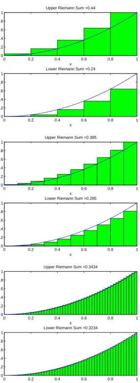
n X k=1 k2=1 6n(n+ 1)(2n+ 1), we get U(f;Pn) = n X k=1 x2k· 1 n = 1 n3 n X k=1 k2= 1 6 1 + 1 n 2 + 1 n and L(f;Pn) = n X k=1 x2k−1· 1 n = 1 n3 n−1 X k=1 k2= 1 6 1− 1 n 2− 1 n . (See Figure 1.18.) It follows that
lim
n→∞U(f;Pn) = limn→∞L(f;Pn) = 1 3, and Theorem 1.17 implies thatx2 is integrable on [0,1] with
Z 1
0
x2dx=1 3.
The fundamental theorem of calculus, Theorem 1.45 below, provides a much easier way to evaluate this integral.
1.5. Integrability of continuous and monotonic functions
The Cauchy criterion leads to the following fundamental result that every continu-ous function is Riemann integrable. To prove this, we use the fact that a continucontinu-ous function oscillates by an arbitrarily small amount on every interval of a sufficiently refined partition.
Theorem 1.19. A continuous function f : [a, b] → R on a compact interval is Riemann integrable.
Proof. A continuous function on a compact set is bounded, so we just need to verify the Cauchy condition in Theorem 1.14.
Letǫ >0. A continuous function on a compact set is uniformly continuous, so there existsδ >0 such that
|f(x)−f(y)|< ǫ
0 0.2 0.4 0.6 0.8 1 0 0.2 0.4 0.6 0.8 1 x y
Upper Riemann Sum =0.44
0 0.2 0.4 0.6 0.8 1 0 0.2 0.4 0.6 0.8 1 x y
Lower Riemann Sum =0.24
0 0.2 0.4 0.6 0.8 1 0 0.2 0.4 0.6 0.8 1 x y
Upper Riemann Sum =0.385
0 0.2 0.4 0.6 0.8 1 0 0.2 0.4 0.6 0.8 1 x y
Lower Riemann Sum =0.285
0 0.2 0.4 0.6 0.8 1 0 0.2 0.4 0.6 0.8 1 x y
Upper Riemann Sum =0.3434
0 0.2 0.4 0.6 0.8 1 0 0.2 0.4 0.6 0.8 1 x y
Lower Riemann Sum =0.3234
Figure 1. Upper and lower Riemann sums for Example 1.18 withn= 5,10,50 subintervals of equal length.
1.5. Integrability of continuous and monotonic functions 13
Choose a partitionP ={I1, I2, . . . , In} of [a, b] such that|Ik|< δ for everyk; for
example, we can takenintervals of equal length (b−a)/nwithn >(b−a)/δ. Since f is continuous, it attains its maximum and minimum values Mk and
mk on the compact interval Ik at points xk and yk in Ik. These points satisfy |xk−yk|< δ, so
Mk−mk=f(xk)−f(yk)<
ǫ b−a. The upper and lower sums off therefore satisfy
U(f;P)−L(f;P) = n X k=1 Mk|Ik| − n X k=1 mk|Ik| = n X k=1 (Mk−mk)|Ik| < ǫ b−a n X k=1 |Ik| < ǫ,
and Theorem 1.14 implies thatf is integrable.
Example 1.20. The function f(x) = x2 on [0,1] considered in Example 1.18 is integrable since it is continuous.
Another class of integrable functions consists of monotonic (increasing or de-creasing) functions.
Theorem 1.21. A monotonic function f : [a, b] → R on a compact interval is Riemann integrable.
Proof. Suppose thatf is monotonic increasing, meaning thatf(x)≤f(y) forx≤
y. LetPn={I1, I2, . . . , In}be a partition of [a, b] intonintervalsIk = [xk−1, xk],
of equal length (b−a)/n, with endpoints xk =a+ (b−a) k n, k= 0,1, . . . , n−1, n. Sincef is increasing, Mk = sup Ik f =f(xk), mk = inf Ik f =f(xk−1).
Hence, summing a telescoping series, we get U(f;Pn)−L(U;Pn) = n X k=1 (Mk−mk) (xk−xk−1) =b−a n n X k=1 [f(xk)−f(xk−1)] =b−a n [f(b)−f(a)].
It follows thatU(f;Pn)−L(U;Pn)→0 asn→ ∞, and Theorem 1.17 implies that
0 0.2 0.4 0.6 0.8 1 0 0.2 0.4 0.6 0.8 1 1.2 x y
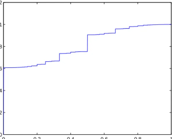
Figure 2. The graph of the monotonic function in Example 1.22 with a count-ably infinite, dense set of jump discontinuities.
The proof for a monotonic decreasing functionf is similar, with sup
Ik
f =f(xk−1), inf Ik
f =f(xk),
or we can apply the result for increasing functions to −f and use Theorem 1.23
below.
Monotonic functions needn’t be continuous, and they may be discontinuous at a countably infinite number of points.
Example 1.22. Let {qk : k ∈N} be an enumeration of the rational numbers in
[0,1) and let (ak) be a sequence of strictly positive real numbers such that
∞ X k=1 ak= 1. Definef : [0,1]→Rby f(x) = X k∈Q(x) ak, Q(x) ={k∈N:qk ∈[0, x)}.
for x > 0, andf(0) = 0. That is, f(x) is obtained by summing the terms in the series whose indiceskcorrespond to the rational numbers 0≤qk< x.
For x = 1, this sum includes all the terms in the series, so f(1) = 1. For every 0 < x < 1, there are infinitely many terms in the sum, since the rationals are dense in [0, x), andf is increasing, since the number of terms increases withx. By Theorem 1.21, f is Riemann integrable on [0,1]. Although f is integrable, it has a countably infinite number of jump discontinuities at every rational number in [0,1), which are dense in [0,1], The function is continuous elsewhere (the proof is left as an exercise).
1.6. Properties of the Riemann integral 15
Figure 2 shows the graph off corresponding to the enumeration
{0,1/2,1/3,2/3,1/4,3/4,1/5,2/5,3/5,4/5,1/6,5/6,1/7, . . .}
of the rational numbers in [0,1) and ak =
6 π2k2.
1.6. Properties of the Riemann integral
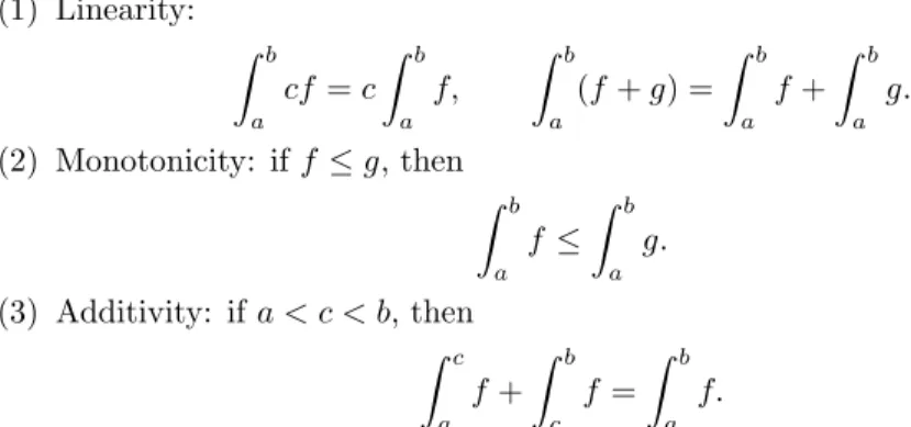
The integral has the following three basic properties. (1) Linearity: Z b a cf=c Z b a f, Z b a (f+g) = Z b a f+ Z b a g. (2) Monotonicity: iff ≤g, then Z b a f ≤ Z b a g. (3) Additivity: if a < c < b, then Z c a f+ Z b c f = Z b a f.
In this section, we prove these properties and derive a few of their consequences. These properties are analogous to the corresponding properties of sums (or convergent series): n X k=1 cak =c n X k=1 ak, n X k=1 (ak+bk) = n X k=1 ak+ n X k=1 bk; n X k=1 ak≤ n X k=1 bk ifak ≤bk; m X k=1 ak+ n X k=m+1 ak= n X k=1 ak.
1.6.1. Linearity. We begin by proving the linearity. First we prove linearity with respect to scalar multiplication and then linearity with respect to sums. Theorem 1.23. Iff : [a, b]→Ris integrable andc∈R, thencf is integrable and
Z b a cf=c Z b a f.
Proof. Suppose thatc≥0. Then for any setA⊂[a, b], we have sup A cf=csup A f, inf A cf =cinfA f,
so U(cf;P) =cU(f;P) for every partitionP. Taking the infimum over the set Π of all partitions of [a, b], we get
U(cf) = inf
Similarly,L(cf;P) =cL(f;P) andL(cf) =cL(f). Iff is integrable, then U(cf) =cU(f) =cL(f) =L(cf),
which shows thatcf is integrable and
Z b a cf=c Z b a f. Now consider−f. Since
sup A (−f) =−inf A f, infA(−f) =−supA f, we have U(−f;P) =−L(f;P), L(−f;P) =−U(f;P). Therefore U(−f) = inf P∈ΠU(−f;P) = infP∈Π[−L(f;P)] =−Psup∈ΠL(f;P) =−L(f), L(−f) = sup P∈Π L(−f;P) = sup P∈Π [−U(f;P)] =− inf P∈ΠU(f;P) =−U(f). Hence,−f is integrable iff is integrable and
Z b a (−f) =− Z b a f.
Finally, ifc <0, thenc=−|c|, and a successive application of the previous results shows thatcf is integrable withRb
a cf=c Rb
af.
Next, we prove the linearity of the integral with respect to sums. If f, g are bounded, thenf +g is bounded and
sup
I (f+g)≤supI f + supI g, infI (f+g)≥infI f+ infI g.
It follows that
osc
I (f+g)≤oscI f+ oscI g,
sof+gis integrable iff,gare integrable. In general, however, the upper (or lower) sum off +g needn’t be the sum of the corresponding upper (or lower) sums off andg. As a result, we don’t get
Z b a (f+g) = Z b a f + Z b a g
simply by adding upper and lower sums. Instead, we prove this equality by esti-mating the upper and lower integrals off+g from above and below by those off andg.
Theorem 1.24. Iff, g: [a, b]→Rare integrable functions, thenf+gis integrable, and Z b a (f+g) = Z b a f+ Z b a g.
1.6. Properties of the Riemann integral 17
Proof. We first prove that if f, g : [a, b] → R are bounded, but not necessarily integrable, then
U(f+g)≤U(f) +U(g), L(f+g)≥L(f) +L(g). Suppose thatP ={I1, I2, . . . , In} is a partition of [a, b]. Then
U(f+g;P) = n X k=1 sup Ik (f+g)· |Ik| ≤ n X k=1 sup Ik f· |Ik|+ n X k=1 sup Ik g· |Ik| ≤U(f;P) +U(g;P).
Let ǫ > 0. Since the upper integral is the infimum of the upper sums, there are partitionsQ,R such that
U(f;Q)< U(f) +ǫ
2, U(g;R)< U(g) + ǫ 2, and ifP is a common refinement ofQandR, then
U(f;P)< U(f) +ǫ 2, U(g;P)< U(g) + ǫ 2. It follows that U(f+g)≤U(f +g;P)≤U(f;P) +U(g;P)< U(f) +U(g) +ǫ.
Since this inequality holds for arbitraryǫ >0, we must haveU(f+g)≤U(f)+U(g). Similarly, we haveL(f+g;P)≥L(f;P) +L(g;P) for all partitionsP, and for everyǫ >0, we getL(f+g)> L(f) +L(g)−ǫ, so L(f+g)≥L(f) +L(g).
For integrable functionsf andg, it follows that
U(f+g)≤U(f) +U(g) =L(f) +L(g)≤L(f+g).
SinceU(f+g)≥L(f+g), we haveU(f +g) =L(f+g) and f+g is integrable. Moreover, there is equality throughout the previous inequality, which proves the
result.
Although the integral is linear, the upper and lower integrals of non-integrable functions are not, in general, linear.
Example 1.25. Definef, g: [0,1]→Rby f(x) = ( 1 ifx∈[0,1]∩Q, 0 ifx∈[0,1]\Q, g(x) = ( 0 ifx∈[0,1]∩Q, 1 ifx∈[0,1]\Q. That is, f is the Dirichlet function and g= 1−f. Then
U(f) =U(g) = 1, L(f) =L(g) = 0, U(f+g) =L(f+g) = 1, so
U(f+g)< U(f) +U(g), L(f+g)> L(f) +L(g).
The product of integrable functions is also integrable, as is the quotient pro-vided it remains bounded. Unlike the integral of the sum, however, there is no way to express the integral of the productR
f gin terms of R
f andR
Theorem 1.26. Iff, g: [a, b]→Rare integrable, thenf g: [a, b]→Ris integrable. If, in addition,g6= 0 and 1/gis bounded, then f /g: [a, b]→Ris integrable. Proof. First, we show that the square of an integrable function is integrable. Iff is integrable, thenf is bounded, with|f| ≤M for someM ≥0. For allx, y∈[a, b], we have
f2(x)−f2(y)
=|f(x) +f(y)| · |f(x)−f(y)| ≤2M|f(x)−f(y)|.
Taking the supremum of this inequality over x, y ∈ I ⊂[a, b] and using Proposi-tion 2.19, we get that
sup I (f2)−inf I (f 2) ≤2M sup I f −inf I f . meaning that osc I (f 2) ≤2Mosc I f.
If follows from Proposition 1.16 thatf2is integrable iff is integrable. Since the integral is linear, we then see from the identity
f g= 1 4
(f +g)2−(f−g)2
thatf g is integrable iff,g are integrable.
In a similar way, ifg6= 0 and|1/g| ≤M, then
1 g(x)− 1 g(y) = |g(x)−g(y)| |g(x)g(y)| ≤M 2 |g(x)−g(y)|. Taking the supremum of this equation overx, y∈I⊂[a, b], we get
sup I 1 g −inf I 1 g ≤M2 sup I g−inf I g ,
meaning that oscI(1/g)≤M2oscIg, and Proposition 1.16 implies that 1/gis
inte-grable ifgis integrable. Thereforef /g=f·(1/g) is integrable. 1.6.2. Monotonicity. Next, we prove the monotonicity of the integral. Theorem 1.27. Suppose thatf, g: [a, b]→Rare integrable andf ≤g. Then
Z b a f ≤ Z b a g.
Proof. First suppose thatf ≥0 is integrable. LetP be the partition consisting of the single interval [a, b]. Then
L(f;P) = inf [a,b]f·(b−a)≥0, so Z b a f ≥L(f;P)≥0.
Iff ≥g, thenh=f−g≥0, and the linearity of the integral implies that
Z b a f− Z b a g= Z b a h≥0,
1.6. Properties of the Riemann integral 19
which proves the theorem.
One immediate consequence of this theorem is the following simple, but useful, estimate for integrals.
Theorem 1.28. Suppose thatf : [a, b]→Ris integrable and M = sup [a,b] f, m= inf [a,b]f. Then m(b−a)≤ Z b a f ≤M(b−a). Proof. Sincem≤f ≤M on [a, b], Theorem 1.27 implies that
Z b a m≤ Z b a f ≤ Z b a M,
which gives the result.
This estimate also follows from the definition of the integral in terms of upper and lower sums, but once we’ve established the monotonicity of the integral, we don’t need to go back to the definition.
A further consequence is the intermediate value theorem for integrals, which states that a continuous function on an interval is equal to its average value at some point.
Theorem 1.29. Iff : [a, b]→ R is continuous, then there exists x∈ [a, b] such that f(x) = 1 b−a Z b a f.
Proof. Sincef is a continuous function on a compact interval, it attains its maxi-mum valueM and its minimum value m. From Theorem 1.28,
m≤b 1 −a
Z b
a
f ≤M.
By the intermediate value theorem,f takes on every value betweenmandM, and
the result follows.
As shown in the proof of Theorem 1.27, given linearity, monotonicity is equiv-alent to positivity,
Z b
a
f ≥0 iff ≥0.
We remark that even though the upper and lower integrals aren’t linear, they are monotone.
Proposition 1.30. Iff, g: [a, b]→Rare bounded functions andf ≤g, then U(f)≤U(g), L(f)≤L(g).
Proof. From Proposition 2.12, we have for every intervalI⊂[a, b] that sup I f ≤sup I g, inf I f ≤infI g.
It follows that for every partitionP of [a, b], we have
U(f;P)≤U(g;P), L(f;P)≤L(g;P).
Taking the infimum of the upper inequality and the supremum of the lower inequal-ity overP, we getU(f)≤U(g) andL(f)≤L(g).
We can estimate the absolute value of an integral by taking the absolute value under the integral sign. This is analogous to the corresponding property of sums:
n X k=1 an ≤ n X k=1 |ak|.
Theorem 1.31. Iff is integrable, then|f|is integrable and
Z b a f ≤ Z b a | f|.
Proof. First, suppose that|f|is integrable. Since
−|f| ≤f ≤ |f|, we get from Theorem 1.27 that
− Z b a | f| ≤ Z b a f ≤ Z b a | f|, or Z b a f ≤ Z b a | f|.
To complete the proof, we need to show that|f|is integrable iff is integrable. Forx, y∈[a, b], the reverse triangle inequality gives
| |f(x)| − |f(y)| | ≤ |f(x)−f(y)|. Using Proposition 2.19, we get that
sup
I |
f| −inf
I |f| ≤supI f−infI f,
meaning that oscI|f| ≤oscIf. Proposition 1.16 then implies that|f|is integrable
iff is integrable.
In particular, we immediately get the following basic estimate for an integral. Corollary 1.32. Iff : [a, b]→Ris integrable
M = sup [a,b]| f|, then Z b a f ≤M(b−a).
1.6. Properties of the Riemann integral 21
1.6.3. Additivity. Finally, we prove additivity. This property refers to addi-tivity with respect to the interval of integration, rather than linearity with respect to the function being integrated.
Theorem 1.33. Suppose that f : [a, b] →Rand a < c < b. Then f is Riemann integrable on [a, b] if and only if it is Riemann integrable on [a, c] and [c, b]. In that case, Z b a f = Z c a f + Z b c f.
Proof. Suppose thatfis integrable on [a, b]. Then, givenǫ >0, there is a partition P of [a, b] such thatU(f;P)−L(f;P)< ǫ. Let P′ =P
∪ {c} be the refinement of P obtained by addingc to the endpoints ofP. (Ifc∈P, thenP′ =P.) Then P′=Q
∪RwhereQ=P′
∩[a, c] andR=P′
∩[c, b] are partitions of [a, c] and [c, b] respectively. Moreover,
U(f;P′) =U(f;Q) +U(f;R), L(f;P′) =L(f;Q) +L(f;R). It follows that
U(f;Q)−L(f;Q) =U(f;P′)−L(f;P′)−[U(f;R)−L(f;R)]
≤U(f;P)−L(f;P)< ǫ,
which proves thatf is integrable on [a, c]. ExchangingQ andR, we get the proof for [c, b].
Conversely, iff is integrable on [a, c] and [c, b], then there are partitions Qof [a, c] andR of [c, b] such that
U(f;Q)−L(f;Q)< ǫ 2, U(f;R)−L(f;R)< ǫ 2. LetP =Q∪R. Then U(f;P)−L(f;P) =U(f;Q)−L(f;Q) +U(f;R)−L(f;R)< ǫ, which proves thatf is integrable on [a, b].
Finally, with the partitionsP,Q,R as above, we have
Z b a f ≤U(f;P) =U(f;Q) +U(f;R) < L(f;Q) +L(f;R) +ǫ < Z c a f+ Z b c f+ǫ. Similarly, Z b a f ≥L(f;P) =L(f;Q) +L(f;R) > U(f;Q) +U(f;R)−ǫ > Z c a f+ Z b c f−ǫ. Sinceǫ >0 is arbitrary, we see thatRb
af =
Rc
af +
Rb
We can extend the additivity property of the integral by defining an oriented Riemann integral.
Definition 1.34. Iff : [a, b]→Ris integrable, wherea < b, anda≤c≤b, then
Z a b f =− Z b a f, Z c c f = 0.
With this definition, the additivity property in Theorem 1.33 holds for all a, b, c ∈R for which the oriented integrals exist. Moreover, if |f| ≤ M, then the estimate in Corollary 1.32 becomes
Z b a f ≤M|b−a|
for alla, b∈R(even ifa≥b).
The oriented Riemann integral is a special case of the integral of a differential form. It assigns a value to the integral of a one-formf dxon an oriented interval.
1.7. Further existence results for the Riemann integral
In this section, we prove several further useful conditions for the existences of the Riemann integral.
First, we show that changing the values of a function at finitely many points doesn’t change its integrability of the value of its integral.
Proposition 1.35. Suppose that f, g : [a, b] → R and f(x) = g(x) except at finitely many points x∈ [a, b]. Thenf is integrable if and only if g is integrable, and in that case
Z b a f = Z b a g.
Proof. It is sufficient to prove the result for functions whose values differ at a single point, sayc∈[a, b]. The general result then follows by induction.
Sincef,g differ at a single point,f is bounded if and only if gis bounded. If f, g are unbounded, then neither one is integrable. If f, g are bounded, we will show that f, g have the same upper and lower integrals because their upper and lower sums differ by an arbitrarily small amount with respect to a partition that is sufficiently refined near the point where the functions differ.
Suppose thatf,g are bounded with|f|,|g| ≤M on [a, b] for someM >0. Let ǫ >0. Choose a partitionP of [a, b] such that
U(f;P)< U(f) +ǫ 2.
LetQ={I1, . . . , In}be a refinement ofP such that|Ik|< δfork= 1, . . . , n, where
δ= ǫ 8M.
1.7. Further existence results for the Riemann integral 23
Thengdiffers fromf on at most two intervals inQ. (There could be two intervals ifcis an endpoint of the partition.) On such an intervalIk we have
sup Ik g−sup Ik f ≤ sup Ik |g|+ sup Ik |f| ≤2M,
and on the remaining intervals, supIkg−supIkf = 0. It follows that
|U(g;Q)−U(f;Q)|<2M·2δ < ǫ 2. Using the properties of upper integrals and refinements, we obtain
U(g)≤U(g;Q)< U(f;Q) +ǫ
2 ≤U(f;P) + ǫ
2 < U(f) +ǫ.
Since this inequality holds for arbitraryǫ >0, we get thatU(g)≤U(f). Exchang-ingf andg, we see similarly thatU(f)≤U(g), soU(f) =U(g).
An analogous argument for lower sums (or an application of the result for upper sums to−f,−g) shows that L(f) =L(g). ThusU(f) =L(f) if and only if U(g) =L(g), in which caseRb
af =
Rb
ag.
Example 1.36. The functionf in Example 1.6 differs from the 0-function at one point. It is integrable and its integral is equal to 0.
The conclusion of Proposition 1.35 can fail if the functions differ at a countably infinite number of points. One reason is that we can turn a bounded function into an unbounded function by changing its values at an infinite number of points. Example 1.37. Definef : [0,1]→Rby
f(x) =
(
n ifx= 1/nforn∈N, 0 otherwise
Thenf is equal to the 0-function except on the countably infinite set{1/n:n∈N}, butf is unbounded and therefore it’s not Riemann integrable.
The result is still false, however, for bounded functions that differ at a countably infinite number of points.
Example 1.38. The Dirichlet function in Example 1.7 is bounded and differs from the 0-function on the countably infinite set of rationals, but it isn’t Riemann integrable.
The Lebesgue integral is better behaved than the Riemann intgeral in this re-spect: two functions that are equal almost everywhere, meaning that they differ on a set of Lebesgue measure zero, have the same Lebesgue integrals. In particu-lar, two functions that differ on a countable set are equal almost everywhere (see Section 1.12).
The next proposition allows us to deduce the integrability of a bounded function on an interval from its integrability on slightly smaller intervals.
Proposition 1.39. Suppose thatf : [a, b]→Ris bounded and integrable on [a, r] for everya < r < b. Thenf is integrable on [a, b] and
Z b a f = lim r→b− Z r a f.
Proof. Sincef is bounded,|f| ≤M on [a, b] for some M >0. Givenǫ >0, let r=b−4Mǫ
(where we assumeǫis sufficiently small that r > a). Sincef is integrable on [a, r], there is a partitionQof [a, r] such that
U(f;Q)−L(f;Q)< ǫ 2.
ThenP =Q∪{b}is a partition of [a, b] whose last interval is [r, b]. The boundedness off implies that sup [r,b] f −inf [r,b]f ≤2M. Therefore U(f;P)−L(f;P) =U(f;Q)−L(f;Q) +sup [r,b] f−inf [r,b]f ·(b−r) < ǫ 2 + 2M ·(b−r) =ǫ,
so f is integrable on [a, b] by Theorem 1.14. Moreover, using the additivity of the integral, we get Z b a f − Z r a f = Z b r f ≤M·(b−r)→0 asr→b−.
An obvious analogous result holds for the left endpoint. Example 1.40. Definef : [0,1]→Rby
f(x) =
(
sin(1/x) if 0< x≤1,
0 ifx= 0.
Thenf is bounded on [0,1]. Furthemore,f is continuous and therefore integrable on [r,1] for every 0< r <1. It follows from Proposition 1.39 that f is integrable on [0,1].
The assumption in Proposition 1.39 thatf is bounded on [a, b] is essential. Example 1.41. The functionf : [0,1]→Rdefined by
f(x) =
(
1/x for 0< x≤1, 0 forx= 0,
is continuous and therefore integrable on [r,1] for every 0 < r < 1, but it’s un-bounded and therefore not integrable on [0,1].
1.7. Further existence results for the Riemann integral 25 0 1 2 3 4 5 6 −1 −0.5 0 0.5 1 x y
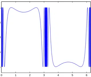
Figure 3. Graph of the Riemann integrable functiony= sin(1/sinx) in Example 1.43.
As a corollary of this result and the additivity of the integral, we prove a generalization of the integrability of continuous functions to piecewise continuous functions.
Theorem 1.42. Iff : [a, b]→Ris a bounded function with finitely many discon-tinuities, thenf is Riemann integrable.
Proof. By splitting the interval into subintervals with the discontinuities off at an endpoint and using Theorem 1.33, we see that it is sufficient to prove the result if f is discontinuous only at one endpoint of [a, b], say at b. In that case, f is continuous and therefore integrable on any smaller interval [a, r] witha < r < b, and Proposition 1.39 implies thatf is integrable on [a, b].
Example 1.43. Definef : [0,2π]→Rby f(x) =
(
sin (1/sinx) if x6= 0, π,2π, 0 ifx= 0, π,2π.
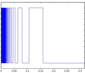
Thenfis bounded and continuous except atx= 0, π,2π, so it is integrable on [0,2π] (see Figure 3). This function doesn’t have jump discontinuities, but Theorem 1.42 still applies. Example 1.44. Definef : [0,1/π]→Rby f(x) = ( sgn [sin (1/x)] ifx6= 1/nπforn∈N, 0 ifx= 0 orx6= 1/nπforn∈N,
0 0.05 0.1 0.15 0.2 0.25 0.3 −1 −0.8 −0.6 −0.4 −0.2 0 0.2 0.4 0.6 0.8 1
Figure 4. Graph of the Riemann integrable functiony= sgn(sin(1/x)) in Example 1.44.
where sgn is the sign function,
sgnx= 1 ifx >0, 0 ifx= 0, −1 ifx <0.
Then f oscillates between 1 and −1 a countably infinite number of times asx→
0+ (see Figure 4). It has jump discontinuities at x = 1/(nπ) and an essential discontinuity atx= 0. Nevertheless, it is Riemann integrable. To see this, note that f is bounded on [0,1] and piecewise continuous with finitely many discontinuities on [r,1] for every 0< r <1. Theorem 1.42 implies that f is Riemann integrable on [r,1], and then Theorem 1.39 implies thatf is integrable on [0,1].
1.8. The fundamental theorem of calculus
In the integral calculus I find much less interesting the parts that involve only substitutions, transformations, and the like, in short, the parts that involve the known skillfully applied mechanics of reducing integrals to algebraic, logarithmic, and circular functions, than I find the careful and profound study of transcendental functions that cannot be reduced to these functions. (Gauss, 1808)
The fundamental theorem of calculus states that differentiation and integration are inverse operations in an appropriately understood sense. The theorem has two parts: in one direction, it says roughly that the integral of the derivative is the original function; in the other direction, it says that the derivative of the integral is the original function.
1.8. The fundamental theorem of calculus 27
In more detail, the first part states that ifF : [a, b]→Ris differentiable with integrable derivative, then
Z b
a
F′(x)dx=F(b)−F(a).
This result can be thought of as a continuous analog of the corresponding identity for sums of differences,
n X
k=1
(Ak−Ak−1) =An−A0.
The second part states that iff : [a, b]→Ris continuous, then d
dx
Z x
a
f(t)dt=f(x).
This is a continuous analog of the corresponding identity for differences of sums,
k X j=1 aj− k−1 X j=1 aj=ak.
The proof of the fundamental theorem consists essentially of applying the iden-tities for sums or differences to the appropriate Riemann sums or difference quo-tients and proving, under appropriate hypotheses, that they converge to the corre-sponding integrals or derivatives.
We’ll split the statement and proof of the fundamental theorem into two parts. (The numbering of the parts as I and II is arbitrary.)
1.8.1. Fundamental theorem I. First we prove the statement about the inte-gral of a derivative.
Theorem 1.45(Fundamental theorem of calculus I). IfF : [a, b]→Ris continuous on [a, b] and differentiable in (a, b) withF′ =f where f : [a, b]
→ R is Riemann integrable, then Z b a f(x)dx=F(b)−F(a). Proof. Let P ={a=x0, x1, x2, . . . , xn−1, xn =b}
be a partition of [a, b]. Then
F(b)−F(a) =
n X
k=1
[F(xk)−F(xk−1)].
The functionF is continuous on the closed interval [xk−1, xk] and differentiable in
the open interval (xk−1, xk) withF′=f. By the mean value theorem, there exists
xk−1< ck< xk such that
F(xk)−F(xk−1) =f(ck)(xk−xk−1).
Sincef is Riemann integrable, it is bounded, and it follows that mk(xk−xk−1)≤F(xk)−F(xk−1)≤Mk(xk−xk−1),
where Mk= sup [xk−1,xk] f, mk = inf [xk−1,xk] f.
Hence, L(f;P) ≤ F(b)−F(a) ≤ U(f;P) for every partition P of [a, b], which implies thatL(f)≤F(b)−F(a)≤U(f). Sincef is integrable,L(f) =U(f) and F(b)−F(a) =Rb
a f.
In Theorem 1.45, we assume that F is continuous on the closed interval [a, b] and differentiable in the open interval (a, b) where its usual two-sided derivative is defined and is equal to f. It isn’t necessary to assume the existence of the right derivative ofF at aor the left derivative atb, so the values off at the endpoints are arbitrary. By Proposition 1.35, however, the integrability off on [a, b] and the value of its integral do not depend on these values, so the statement of the theorem makes sense. As a result, we’ll sometimes abuse terminology, and say that “F′ is integrable on [a, b]” even if it’s only defined on (a, b).
Theorem 1.45 imposes the integrability ofF′as a hypothesis. Every functionF that is continuously differentiable on the closed interval [a, b] satisfies this condition, but the theorem remains true even if F′ is a discontinuous, Riemann integrable function. Example 1.46. DefineF : [0,1]→Rby F(x) = ( x2sin(1/x) if 0< x≤1, 0 ifx= 0.
Then F is continuous on [0,1] and, by the product and chain rules, differentiable in (0,1]. It is also differentiable — but not continuously differentiable — at 0, with F′(0+) = 0. Thus,
F′(x) =
(
−cos (1/x) + 2xsin (1/x) if 0< x≤1,
0 ifx= 0.
The derivativeF′ is bounded on [0,1] and discontinuous only at one point (x= 0), so Theorem 1.42 implies that F′ is integrable on [0,1]. This verifies all of the hypotheses in Theorem 1.45, and we conclude that
Z 1
0
F′(x)dx= sin 1.
There are, however, differentiable functions whose derivatives are unbounded or so discontinuous that they aren’t Riemann integrable.
Example 1.47. Define F : [0,1]→ Rby F(x) = √x. ThenF is continuous on [0,1] and differentiable in (0,1], with
F′(x) = 1
2√x for 0< x≤1.
This function is unbounded, soF′ is not Riemann integrable on [0,1], however we define its value at 0, and Theorem 1.45 does not apply.
1.8. The fundamental theorem of calculus 29
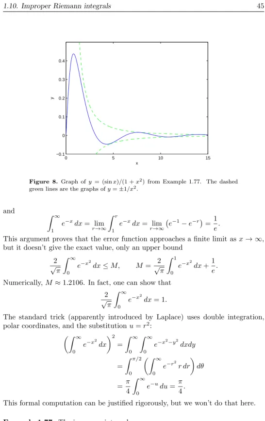
We can, however, interpret the integral ofF′on [0,1] as an improper Riemann integral. The functionF is continuously differentiable on [ǫ,1] for every 0< ǫ <1, so Z 1 ǫ 1 2√xdx= 1− √ ǫ. Thus, we get the improper integral
lim ǫ→0+ Z 1 ǫ 1 2√xdx= 1.
The construction of a function with a bounded, non-integrable derivative is more involved. It’s not sufficient to give a function with a bounded derivative that is discontinuous at finitely many points, as in Example 1.46, because such a function is Riemann integrable. Rather, one has to construct a differentiable function whose derivative is discontinuous on a set of nonzero Lebesgue measure; we won’t give an example here.
Finally, we remark that Theorem 1.45 remains valid for the oriented Riemann integral, since exchangingaandb reverses the sign of both sides.
1.8.2. Fundamental theorem of calculus II. Next, we prove the other direc-tion of the fundamental theorem. We will use the following result, of independent interest, which states that the average of a continuous function on an interval ap-proaches the value of the function as the length of the interval shrinks to zero. The proof uses a common trick of taking a constant inside an average.
Theorem 1.48. Suppose thatf : [a, b]→Ris integrable on [a, b] and continuous ata. Then lim h→0+ 1 h Z a+h a f(x)dx=f(a). Proof. Ifkis a constant, we have
k= 1 h
Z a+h
a
k dx.
(That is, the average of a constant is equal to the constant.) We can therefore write 1 h Z a+h a f(x)dx−f(a) = 1 h Z a+h a [f(x)−f(a)]dx. Letǫ >0. Sincef is continuous ata, there existsδ >0 such that
|f(x)−f(a)|< ǫ for a≤x < a+δ. It follows that if 0< h < δ, then
1 h Z a+h a f(x)dx−f(a) ≤h1 · sup a≤a≤a+h| f(x)−f(a)| ·h≤ǫ,
A similar proof shows that iff is continuous atb, then lim h→0+ 1 h Z b b−h f =f(b), and iff is continuous ata < c < b, then
lim h→0+ 1 2h Z c+h c−h f =f(c).
More generally, if{Ih:h >0}is any collection of intervals withc∈Ih and|Ih| →0
ash→0+, then lim h→0+ 1 |Ih| Z Ih f =f(c).
The assumption in Theorem 1.48 thatf is continuous at the point about which we take the averages is essential.
Example 1.49. Letf :R→Rbe the sign function f(x) = 1 ifx >0, 0 ifx= 0, −1 ifx <0. Then lim h→0+ 1 h Z h 0 f(x)dx= 1, lim h→0+ 1 h Z 0 −h f(x)dx=−1,
and neither limit is equal to f(0). In this example, the limit of the symmetric averages lim h→0+ 1 2h Z h −h f(x)dx= 0
is equal tof(0), but this equality doesn’t hold if we changef(0) to a nonzero value, since the limit of the symmetric averages is still 0.
The second part of the fundamental theorem follows from this result and the fact that the difference quotients ofF are averages off.
Theorem 1.50(Fundamental theorem of calculus II). Suppose thatf : [a, b]→R
is integrable andF : [a, b]→Ris defined by F(x) =
Z x
a
f(t)dt.
ThenF is continuous on [a, b]. Moreover, iff is continuous ata≤c≤b, thenF is differentiable atcandF′(c) =f(c).
Proof. First, note that Theorem 1.33 implies thatf is integrable on [a, x] for every a≤x≤b, soF is well-defined. Since f is Riemann integrable, it is bounded, and
|f| ≤M for some M ≥0. It follows that
|F(x+h)−F(x)|= Z x+h x f(t)dt ≤M|h|,
1.8. The fundamental theorem of calculus 31 Moreover, we have F(c+h)−F(c) h = 1 h Z c+h c f(t)dt.
It follows from Theorem 1.48 that iff is continuous at c, thenF is differentiable atc with F′(c) = lim h→0 F(c+h) −F(c) h = lim h→0 1 h Z c+h c f(t)dt=f(c),
where we use the appropriate right or left limit at an endpoint.
The assumption thatf is continuous is needed to ensure thatFis differentiable. Example 1.51. If f(x) = ( 1 forx≥0, 0 forx <0, then F(x) = Z x 0 f(t)dt= ( x forx≥0, 0 forx <0.
The function F is continuous but not differentiable at x= 0, where f is discon-tinuous, since the left and right derivatives of F at 0, given by F′(0−) = 0 and F′(0+) = 1, are different.
1.8.3. Consequences of the fundamental theorem. The first part of the fun-damental theorem, Theorem 1.45, is the basic computational tool in integration. It allows us to compute the integral of of a functionf if we can find an antiderivative; that is, a functionF such thatF′=f. There is no systematic procedure for find-ing antiderivatives. Moreover, even if one exists, an antiderivative of an elementary function (constructed from power, trigonometric, and exponential functions and their inverses) may not be — and often isn’t — expressible in terms of elementary functions.
Example 1.52. Forp= 0,1,2, . . ., we have d dx 1 p+ 1x p+1 =xp, and it follows that
Z 1
0
xpdx= 1 p+ 1.
We remark that once we have the fundamental theorem, we can use the definition of the integral backwards to evaluate a limit such as
lim n→∞ " 1 np+1 n X k=1 kp # = 1 p+ 1,
since the sum is the upper sum ofxp on a partition of [0,1] intonintervals of equal
Two important general consequences of the first part of the fundamental theo-rem are integration by parts and substitution (or change of variable), which come from inverting the product rule and chain rule for derivatives, respectively. Theorem 1.53 (Integration by parts). Suppose thatf, g: [a, b]→Rare continu-ous on [a, b] and differentiable in (a, b), andf′,g′ are integrable on [a, b]. Then
Z b a f g′dx=f(b)g(b)−f(a)g(a)− Z b a f′g dx.
Proof. The function f g is continuous on [a, b] and, by the product rule, differen-tiable in (a, b) with derivative
(f g)′=f g′+f′g.
Since f,g, f′, g′ are integrable on [a, b], Theorem 1.26 implies that f g′, f′g, and (f g)′, are integrable. From Theorem 1.45, we get that
Z b a f g′dx+Z b a f′g dx=Z b a f′g dx=f(b)g(b) −f(a)g(a),
which proves the result.
Integration by parts says that we can move a derivative from one factor in an integral onto the other factor, with a change of sign and the appearance of a boundary term. The product rule for derivatives expresses the derivative of a product in terms of the derivatives of the factors. By contrast, integration by parts doesn’t give an explicit expression for the integral of a product, it simply replaces one integral by another. This can sometimes be used to simplify an integral and evaluate it, but the importance of integration by parts goes far beyond its use as an integration technique.
Example 1.54. Forn= 0,1,2,3, . . ., let In(x) =
Z x
0
tne−tdt.
Ifn≥1, integration by parts withf(t) =tn andg′(t) =e−tgives
In(x) =−xne−x+n Z x 0 tn−1e−tdt= −xne−x+nI n−1(x).
Also, by the fundamental theorem, I0(x) =
Z x
0
e−tdt= 1−e−x.
It then follows by induction that In(x) =n! " 1−e−x n X k=0 xk k! # , where, as usual, 0! = 1.
Since xke−x → 0 as x → ∞ for every k = 0,1,2, . . ., we get the improper
integral Z ∞ 0 tne−tdt= lim r→∞ Z r 0 tne−tdt=n!.
1.8. The fundamental theorem of calculus 33
This formula suggests an extension of the factorial function to complex numbers z ∈C, called the Gamma function, which is defined forℜz > 0 by the improper, complex-valued integral
Γ(z) =
Z ∞
0
tz−1e−tdt.
In particular, Γ(n) = (n−1)! forn∈N. The Gama function is an important special function, which is studied further in complex analysis.
Next we consider the change of variable formula for integrals.
Theorem 1.55 (Change of variable). Suppose thatg:I→Rdifferentiable on an open intervalI and g′ is integrable onI. Let J =g(I). If f :J
→Rcontinuous, then for everya, b∈I,
Z b a f(g(x))g′(x)dx= Z g(b) g(a) f(u)du. Proof. Let F(x) = Z x a f(u)du.
Since f is continuous, Theorem 1.50 implies that F is differentiable in J with F′=f. The chain rule implies that the compositionF
◦g:I→Ris differentiable inI, with
(F◦g)′(x) =f(g(x))g′(x).
This derivative is integrable on [a, b] sincef◦g is continuous and g′ is integrable. Theorem 1.45, the definition of F, and the additivity of the integral then imply that Z b a f(g(x))g′(x)dx= Z b a (F◦g)′dx =F(g(b))−F(g(a)) = Z g(b) g(a) F′(u)du,
which proves the result.
A continuous function maps an interval to an interval, and it is one-to-one if and only if it is strictly monotone. An increasing function preserves the orientation of the interval, while a decreasing function reverses it, in which case the integrals are understood as appropriate oriented integrals. There is no assumption in this theorem thatgis invertible, and the result remains valid ifg is not monotone. Example 1.56. For everya >0, the increasing, differentiable functiong:R→R
defined by g(x) = x3 maps (−a, a) one-to-one and onto (−a3, a3) and preserves orientation. Thus, iff : [−a, a]→Ris continuous,
Z a −a f(x3)·3x2dx= Z a3 −a3 f(u)du.
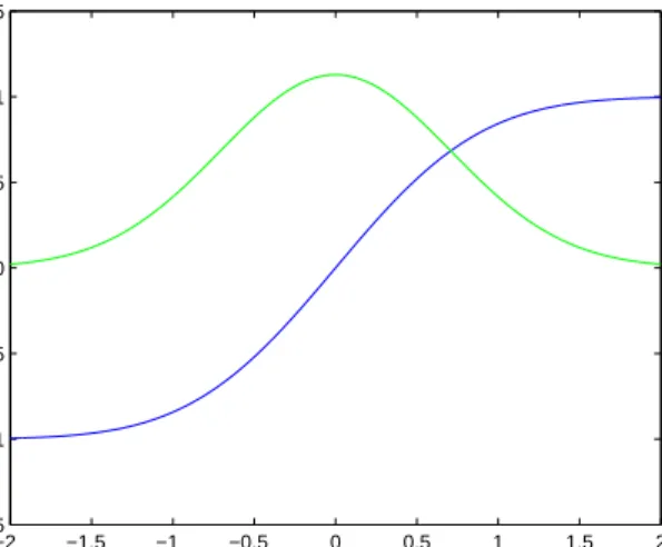
−2 −1.5 −1 −0.5 0 0.5 1 1.5 2 −1.5 −1 −0.5 0 0.5 1 1.5 x y
Figure 5. Graphs of the error functiony =F(x) (blue) and its derivative,
the Gaussian functiony=f(x) (green), from Example 1.58.
The decreasing, differentiable function g : R → R defined by g(x) = −x3 maps (−a, a) one-to-one and onto (−a3, a3) and reverses orientation. Thus,
Z a −a f(−x3)·(−3x2)dx= Z −a3 a3 f(u)du=− Z a3 −a3 f(u)du.
The non-monotone, differentiable function g :R →Rdefined by g(x) =x2 maps (−a, a) onto [0, a2). It is two-to-one, except at x = 0. The change of variables formula gives Z a −a f(x2)·2x dx= Z a2 a2 f(u)du= 0.
The contributions to the original integral from [0, a] and [−a,0] cancel since the integrand is an odd function ofx.
One consequence of the second part of the fundamental theorem, Theorem 1.50, is that every continuous function has an antiderivative, even if it can’t be expressed explicitly in terms of elementary functions. This provides a way to define transcen-dental functions as integrals of elementary functions.
Example 1.57. One way to define the logarithm ln : (0,∞) → R in terms of algebraic functions is as the integral
lnx=
Z x
1 1 tdt.
The integral is well-defined for every 0 < x < ∞ since 1/t is continuous on the interval [1, x] (or [x,1] if 0< x <1). The usual properties of the logarithm follow from this representation. We have (lnx)′ = 1/x by definition, and, for example, making the substitution s = xt in the second integral in the following equation,
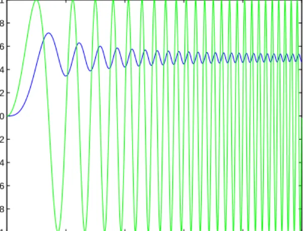
1.8. The fundamental theorem of calculus 35 0 2 4 6 8 10 −1 −0.8 −0.6 −0.4 −0.2 0 0.2 0.4 0.6 0.8 1 x y
Figure 6. Graphs of the Fresnel integraly =S(x) (blue) and its derivative
y= sin(πx2/2) (green) from Example 1.59.
whendt/t=ds/s, we get lnx+ lny= Z x 1 1 t dt+ Z y 1 1 t dt= Z x 1 1 tdt+ Z xy x 1 sds= Z xy 1 1 tdt= ln(xy). We can also define many non-elementary functions as integrals.
Example 1.58. The error function erf(x) =√2
π
Z x
0
e−t2dt is an anti-derivative onRof the Gaussian function
f(x) = √2
πe −x2
.
The error function isn’t expressible in terms of elementary functions. Nevertheless, it is defined as a limit of Riemann sums for the integral. Figure 5 shows the graphs off andF. The name “error function” comes from the fact that the probability of a Gaussian random variable deviating by more than a given amount from its mean can be expressed in terms ofF. Error functions also arise in other applications; for example, in modeling diffusion processes such as heat flow.
Example 1.59. The Fresnel sine functionS is defined by S(x) = Z x 0 sin πt2 2 dt.
The function S is an antiderivative of sin(πt2/2) on R(see Figure 6), but it can’t be expressed in terms of elementary functions. Fresnel integrals arise, among other places, in analysing the diffraction of waves, such as light waves. From the perspec-tive of complex analysis, they are closely related to the error function through the Euler formulaeiθ= cosθ+isinθ.
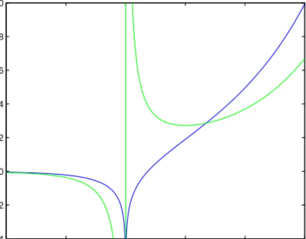
−2 −1 0 1 2 3 −4 −2 0 2 4 6 8 10
Figure 7. Graphs of the exponential integraly= Ei(x) (blue) and its
deriv-ativey=ex
/x(green) from Example 1.60.
Example 1.60. The exponential integral Ei is a non-elementary function defined by Ei(x) = Z x −∞ et t dt.
Its graph is shown in Figure 7. This integral has to be understood, in general, as an improper, principal value integral, and the function has a logarithmic singularity at x= 0 (see Example 1.83 below for further explanation). The exponential integral arises in physical applications such as heat flow and radiative transfer. It is also related to the logarithmic integral
li(x) =
Z x
0 dt lnt
by li(x) = Ei(lnx). The logarithmic integral is important in number theory, and it gives an asymptotic approximation for the number of primes less thanxasx→ ∞. Roughly speaking, the density of the primes near a large numberxis close to 1/lnx. Discontinuous functions may or may not have an antiderivative, and typically they don’t. Darboux proved that every functionf : (a, b)→Rthat is the derivative of a function F : (a, b) → R, where F′ = f at every point of (a, b), has the intermediate value property. That is, ifa < c < d < b, then for every y between f(c) andf(d) there exists anxbetweenc anddsuch thatf(x) =y. A continuous derivative has this property by the intermediate value theorem, but a discontinuous derivative also has it. Thus, functions without the intermediate value property, such as ones with a jump discontinuity or the Dirichlet function, don’t have an antiderivative. For example, the functionFin Example 1.51 is not an antiderivative of the step functionf onRsince it isn’t differentiable at 0.
In dealing with functions that are not continuously differentiable, it turns out to be more useful to abandon the idea of a derivative that is defined pointwise
1.9. Integrals and sequences of functions 37
everywhere (pointwise values of discontinuous functions are somewhat arbitrary) and introduce the notion of a weak derivative. We won’t define or study weak derivatives here.
1.9. Integrals and sequences of functions
A fundamental question that arises throughout analysis is the validity of an ex-change in the order of limits. Some sort of condition is always required.
In this section, we consider the question of when the convergence of a sequence of functions fn →f implies the convergence of their integralsRfn →Rf. There
are many inequivalent notions of the convergence of functions. The two we’ll discuss here are pointwise and uniform convergence.
Recall that if fn, f : A → R, then fn → f pointwise on A as n → ∞ if
fn(x)→f(x) for everyx∈A. On the other hand, fn →f uniformly onA if for
everyǫ >0 there existsN ∈Nsuch that
n > N implies that |fn(x)−f(x)|< ǫ for everyx∈A.
Equivalently,fn→f uniformly onAifkfn−fk →0 asn→ ∞, where kfk= sup{|f(x)|:x∈A}
denotes the sup-norm of a function f : A → R. Uniform convergence implies pointwise convergence, but not conversely.
As we show first, the Riemann integral is well-behaved with respect to uniform convergence. The drawback to uniform convergence is that it’s a strong form of convergence, and we often want to use a weaker form, such as pointwise convergence, in which case the Riemann integral may not be suitable.
1.9.1. Uniform convergence. The uniform limit of continuous functions is con-tinuous and therefore integrable. The next result shows, more generally, that the uniform limit of integrable functions is integrable. Furthermore, the limit of the integrals is the integral of the limit.
Theorem 1.61. Suppose thatfn: [a, b]→Ris Riemann integrable for eachn∈N
andfn→f uniformly on [a, b] asn→ ∞. Thenf : [a, b]→Ris Riemann integrable
on [a, b] and Z b a f = lim n→∞ Z b a fn.
Proof. The uniform limit of bounded functions is bounded, sof is bounded. The main statement we need to prove is thatf is integrable.
Letǫ >0. Sincefn →f uniformly, there is anN ∈Nsuch that ifn > N then
fn(x)−
ǫ
b−a < f(x)< fn(x) + ǫ
b−a for alla≤x≤b. It follows from Proposition 1.30 that
L fn− ǫ b−a ≤L(f), U(f)≤U fn+ ǫ b−a .
Since fn is integrable and upper integrals are greater than lower integrals, we get that Z b a fn−ǫ≤L(f)≤U(f)≤ Z b a fn+ǫ,
which implies that
0≤U(f)−L(f)≤2ǫ.
Sinceǫ >0 is arbitrary, we conclude thatL(f) =U(f), sof is integrable. Moreover, it follows that for alln > N we have
Z b a fn− Z b a f ≤ǫ, which shows thatRb
a fn→ Rb
a f asn→ ∞.
Once we know that the uniform limit of integrable functions is integrable, the convergence of the integrals also follows directly from the estimate
Z b a fn− Z b a f = Z b a (fn−f) ≤ kfn−fk ·(b−a)→0 asn→ ∞.
Example 1.62. The functionfn : [0,1]→Rdefined by
fn(x) = n+ cosx nex+ sinx converges uniformly on [0,1] to f(x) =e−x, since for 0≤x≤1 n+ cosx nex+ sinx−e −x = cosx−e−xsinx nex+ sinx ≤ 2 n. It follows that lim n→∞ Z 1 0 n+ cosx nex+ sinxdx= Z 1 0 e−xdx= 1 −1 e. Example 1.63. Every power series
f(x) =a0+a1x+a2x2+· · ·+anxn+. . .
with radius of convergenceR >0 converges uniformly on compact intervals inside the interval|x|< R, so we can integrate it term-by-term to get
Z x 0 f(t)dt=a0x+1 2a1x 2+1 3a2x 3+ · · ·+ 1 n+ 1anx n+1+. . . for |x|< R. As one example, if we integrate the geometric series
1
1−x= 1 +x+x 2+
· · ·+xn+. . . for|x|<1, we get a power series for ln,
ln 1 1−x =x+1 2x 2+1 3x 3 · · ·+1 nx n+. . . for |x|<1.
1.9. Integrals and sequences of functions 39
For instance, takingx= 1/2, we get the rapidly convergent series ln 2 = ∞ X n=1 1 n2n
for the irrational number ln 2≈0.6931. This series was known and used by Euler. Although we can integrate uniformly convergent sequences, we cannot in gen-eral differentiate them. In fact, it’s often easier to prove results about the conver-gence of derivatives by using results about the converconver-gence of integrals, together with the fundamental theorem of calculus. The following theorem provides suffi-cient conditions forfn→f to imply thatfn′ →f′.
Theorem 1.64. Letfn: (a, b)→Rbe a sequence of differentiable functions whose
derivativesf′
n: (a, b)→Rare integrable on (a, b). Suppose thatfn→f pointwise
andf′
n→guniformly on (a, b) asn→ ∞, whereg: (a, b)→Ris continuous. Then
f : (a, b)→Ris continuously differentiable on (a, b) andf′=g. Proof. Choose some point a < c < b. Since f′
n is integrable, the fundamental
theorem of calculus, Theorem 1.45, implies that fn(x) =fn(c) +
Z x
c
f′
n fora < x < b.
Sincefn →f pointwise andfn′ →g uniformly on [a, x], we find that
f(x) =f(c) +
Z x
c
g.
Since g is continuous, the other direction of the fundamental theorem, Theo-rem 1.50, implies thatf is differentiable in (a, b) andf′ =g.
In particular, this theorem shows that the limit of a uniformly convergent se-quence of continuously differentiable functions whose derivatives converge uniformly is also continuously differentiable.
The key assumption in Theorem 1.64 is that the derivatives f′
n converge
uni-formly, not just pointwise; the result is false if we only assume pointwise convergence of thef′
n. In the proof of the theorem, we only use the assumption thatfn(x)
con-verges at a single pointx=c. This assumption together with the assumption that f′
n →guniformly implies that fn→f pointwise (and, in fact, uniformly) where
f(x) = lim
n→∞fn(c) +
Z x
c
g.
Thus, the theorem remains true if we replace the assumption thatfn→f pointwise
on (a, b) by the weaker assumption that limn→∞fn(c) exists for some c ∈ (a, b).
This isn’t an important change, however, because the restrictive assumption in the theorem is the uniform convergence of the derivatives f′
n, not the pointwise (or
uniform) convergence of the functionsfn.
The assumption that g = limf′
n is continuous is needed to show the
differ-entiability of f by the fundamental theorem, but the result result true even ifg isn’t continuous. In that case, however, a different (and more complicated) proof is required.