2010
Comparison of encoding schemes for symbolic
model checking of bounded petri nets
Nishtha Arora
Iowa State UniversityFollow this and additional works at:
https://lib.dr.iastate.edu/etd
Part of the
Computer Sciences Commons
This Thesis is brought to you for free and open access by the Iowa State University Capstones, Theses and Dissertations at Iowa State University Digital Repository. It has been accepted for inclusion in Graduate Theses and Dissertations by an authorized administrator of Iowa State University Digital Repository. For more information, please [email protected].
Recommended Citation
Arora, Nishtha, "Comparison of encoding schemes for symbolic model checking of bounded petri nets" (2010).Graduate Theses and Dissertations. 11511.
by
Nishtha Arora
A thesis submitted to the graduate faculty
in partial fulfillment of the requirements for the degree of MASTER OF SCIENCE
Major: Computer Science
Program of Study Committee: Andrew S. Miner, Major Professor
Samik Basu Robyn Lutz
Iowa State University Ames, Iowa
2010
DEDICATION
I would like to dedicate this thesis to my parents who have been a source of inspiration and encouragement to me all throughout my life. A very special thanks to Prof. Andrew Miner for his constant support and guidance. I learnt a lot from him and would like to thank him from all my heart. I would also like to take this opportunity to thank Junaid Babar and my committee members, Prof. Samik Basu and Prof. Robyn Lutz for their help and support.
Thanks to my siblings for their unconditional love that has helped me succeed at every step. Finally, I would like to thank my friend Shantanu, who instilled in me the confidence that I am capable of doing anything I put my mind to.
TABLE OF CONTENTS
LIST OF TABLES . . . v
LIST OF FIGURES . . . vii
ABSTRACT . . . ix
CHAPTER 1. OVERVIEW . . . 1
1.1 Introduction . . . 1
CHAPTER 2. REVIEW OF LITERATURE . . . 3
2.1 Overview . . . 3
2.2 Decision Diagrams . . . 3
2.2.1 Binary Decision Diagrams . . . 4
2.2.2 Algebraic Decision Diagrams . . . 5
2.2.3 Multi Valued Decision Diagrams . . . 6
2.2.4 Matrix Diagrams . . . 9
2.2.5 Operations on DDs . . . 11
2.3 Petri Nets . . . 14
2.4 Building Transition relation and Reachability set . . . 20
2.5 Model Checking . . . 22
CHAPTER 3. ENCODING SCHEMES . . . 29
3.1 Overview . . . 29
3.2 One-hot Encoding Scheme . . . 29
3.3 Logarithmic encoding . . . 32
3.5 Proposed Encoding Scheme - K-Hot Encoding . . . 39
3.5.1 Encoding Forkjoin model withkas 2 . . . 42
3.5.2 Encoding Forkjoin model withkas 3 . . . 42
CHAPTER 4. RESULTS . . . 44 4.1 Overview . . . 44 4.2 Experimental setup . . . 44 4.2.1 CuddImpl . . . 45 4.2.2 MeddlyImpl . . . 46 4.3 Fork-join model . . . 47
4.4 Dining philosopher model . . . 51
4.5 Swaps model . . . 55
4.6 Kanban model . . . 58
4.7 Tiles model . . . 62
4.8 Performance in computing CTL formulas . . . 66
4.9 Discussion . . . 68
CHAPTER 5. SUMMARY AND FUTURE WORK . . . 70
LIST OF TABLES
Table 3.1 Encoding for placep1 . . . 31
Table 3.2 Part of the transition relation for the Petri net shown in Figure 2.26 for N = 9 . . . 32
Table 3.3 Place p1 encoded using variables xp1,0,xp1,1,xp1,2 and xp1,3 . . . 34
Table 3.4 Part of the Transition relation of Petri net in Figure 2.26 withN = 9 . 35 Table 3.5 Representing number of tokens at a place with bound 9 using 2-hot . . 41
Table 3.6 Representing number of tokens at a place with bound 9 using 3-hot . . 41
Table 3.7 Part of the transition relation for Figure 2.26 withN = 9 using k-hot encoding with kas 2 . . . 42
Table 3.8 Part of the Transition relation for Figure 2.26 with N = 9 using k-hot encoding with kas 3 . . . 43
Table 4.1 Properties of Fork-join model . . . 48
Table 4.2 Fork-join in CuddImpl . . . 49
Table 4.3 Fork-join in MeddlyImpl . . . 50
Table 4.4 Properties of Philosophers model . . . 53
Table 4.5 Philosophers model in CuddImpl . . . 53
Table 4.6 Philosophers model in MeddlyImpl . . . 54
Table 4.7 Properties of Swaps model . . . 55
Table 4.8 Swaps model in CuddImpl . . . 56
Table 4.9 Swaps model in MeddlyImpl . . . 57
Table 4.10 Properties of Kanban model . . . 59
Table 4.12 Kanban model in MeddlyImpl . . . 61
Table 4.13 Properties of Tiles model . . . 62
Table 4.14 Tiles model in CuddImpl . . . 64
Table 4.15 Tiles model in MeddlyImpl . . . 65
LIST OF FIGURES
Figure 2.1 BDD representing functionf =ab0+a0bc. . . . 4
Figure 2.2 Function f defined using a truth table on the right and ADD represent-ing this function on the left . . . 6
Figure 2.3 Example of an MDD . . . 7
Figure 2.4 MDD on the left shows the quasi-reduced form of the MDD in Figure 2.3 and the one on the right shows its fully-reduced form. . . 8
Figure 2.5 Truth table for functionf on the left and its MTMDD representation on the right. . . 8
Figure 2.6 MTMDD on the left shows the quasi-reduced form of the MTMDD in Figure 2.5 and the one on the right shows its fully-reduced form. . . . 9
Figure 2.7 Identity reduced MxD [14] . . . 10
Figure 2.8 Apply method to computev1 ⊕v2 . . . 12
Figure 2.9 BDD for¬(x1∧x3) on the left andx2∧x3 on the right [4] . . . 13
Figure 2.10 BDD for¬(x1∧x3)∨(x2∧x3)[4] . . . 14
Figure 2.11 Petri Net . . . 15
Figure 2.12 Petri Net with inhibitor arcs . . . 15
Figure 2.13 BDD for the marking setM={[100],[011],[101]} . . . 18
Figure 2.14 Petri net for Forkjoin Model . . . 18
Figure 2.15 Reachability graph for Forkjoin model withN = 1 . . . 19
Figure 2.16 Building enabling relation . . . 20
Figure 2.17 Building firing relation . . . 21
Figure 2.19 Algorithm for building Reachability Decision Diagram . . . 22
Figure 2.20 MxD for enabling expression on the left, firing expression in the middle and transitiont on the right . . . 23
Figure 2.21 M, s|=AGg and M, s|=AFg . . . 25
Figure 2.22 M, s|=EFg and M, s|=EGg . . . 25
Figure 2.23 Algorithm for CTL formulaEXp . . . 26
Figure 2.24 Algorithm for CTL formulaEpUq . . . 26
Figure 2.25 Algorithm for CTL formulaEGp . . . 27
Figure 2.26 Reachability graph of the Petri net of Figure 2.14 . . . 28
Figure 3.1 MDD forx > y on the left and the corresponding BDD on the right . . 36
Figure 3.2 MDD representing the initial state of the Petri net shown in Figure 2.26 withN = 9 . . . 36
Figure 3.3 MxD representing a part of the transition relation of the PN shown in Figure 2.26 withN = 9 . . . 37
Figure 3.4 MDD representing a part of the reachability set of the PN shown in Figure 2.26 withN = 9 . . . 38
Figure 3.5 Encoding placep using k-hot encoding . . . . 40
Figure 4.1 3 Dining philosophers model . . . 52
Figure 4.2 Swaps-3 model . . . 55
Figure 4.3 Kanban model . . . 58
ABSTRACT
Petri nets are a graph based formalism used for modelling concurrent systems. Binary Decision Diagrams or Multi-Valued Decision Diagrams can be used in the analysis of systems modelled by Petri nets. An encoding scheme is required to be able to map the Petri net state to decision diagram values. Various encodings like One-hot scheme, Logarithmic scheme and Mdd scheme exist for this purpose. This thesis compares the performance of the existing encodings based on time and space taken to represent and analyze the system modelled as Petri net. It also introduces and compares a new encoding scheme called k-hot encoding and shows a gradual improvement in performance of the scheme with increasing values of k. The process of analyzing properties like deadlock and starvation is explained and a comparison is made between the encoding schemes based on the time taken by each to analyze these properties.
CHAPTER 1. OVERVIEW
1.1 Introduction
The software or hardware systems used nowadays are mostly huge and complicated. Thus, modelling and analyzing such systems has become complicated too. A representation for such a system can be used to evaluate the possible states the system can be in. One of the problems with representing such systems is the possibility of exponential growth in the number of states with the size of the system. This problem is well known as theState Explosion problem. The state explosion problem restricts huge concurrent systems from being represented and thus analyzing them or verifying properties for such system has become an issue. A lot of research work has been done in this context to make it possible to represent bigger and bigger systems efficiently and in a compact manner.
Efficiently modelling a system requires taking less space and time in representing the sys-tem. Decision Diagrams are used as they are capable of representing large systems in the form of compact data structures. In order to efficiently model concurrent systems, firstly a compact representation is chosen, secondly a good encoding scheme for the representation is selected and lastly a good enough ordering for the encoding variables is used.
The contributions of this thesis are as follows:
• This thesis evaluates and compares the existing encoding schemes(for Petri nets) namely One-hot scheme, Logarithmic scheme and MDD scheme based on their performance. The metrics used for evaluation are time and space taken to represent and analyze well known concurrent systems.
and performs better with every increasing value of k.
• A comparison is made between the existing schemes and the newk-hot scheme using the same time and space metrics.
• Some of the systems are analyzed for properties like deadlock and starvation. This anal-ysis is done using the existing and new schemes. A comparison is made between the time taken by each encoding scheme to analyze the given properties on the system.
Choosing the right encoding scheme is important for efficiently modelling a system, hence this evaluation helps in deciding the appropriate scheme for a system.
The remainder of this thesis is organized as follows. Chapter 2 of this thesis gives an introduction to the basic concepts like Decision Diagrams, Petri nets and Model checking. Chapter 3 explains in detail the existing encoding schemes. Towards the end, this chapter introduces a new encoding scheme and explains it in detail with the help of the Fork-join Petri net model. Chapter 4 compares the existing and proposed encoding schemes based on several metrics and lists the advantages and disadvantages of each scheme. The results of this comparison conclude when to use each encoding scheme. Chapter 5 summarizes the results of this thesis and describes some of the open problems in this context.
CHAPTER 2. REVIEW OF LITERATURE
2.1 Overview
This chapter introduces some of the key concepts related to modelling concurrent systems. Decision Diagrams have been popular data structures for representing huge concurrent systems. They generally provide a compact representation for sets of states and are discussed in detail in Section 2.2. Decision Diagrams can be further narrowed down to Binary Decision Diagrams, Multi Valued Decision Diagrams or more. Some of these types are also dicussed in this section. Section 2.3 introduces Petri Nets, which provide a front end used for modelling and analyzing concurrent systems. Lastly, Section 2.5 introduces Symbolic Model Checking [17]. Model checking refers to the process of verifying if a given model of the system satisfies a system property or not. Traditionally, the process of model checking consists of building the state graph and using temporal logic to verify a system property for that graph. In Symbolic Model Checking, BDD’s are used for representing the state graph of the system.
2.2 Decision Diagrams
Decision Diagrams(DD) are used for representing points of decision and their possible results. It is possible to calculate the probability of an outcome/result using a DD [7]. They can be used for calculating and comparing the total cost for various alternative decisions and thus help in decision making [7]. Some important and popular types of Decision Diagrams are discussed below.
Binary Decision Diagrams(BDD’s) [5, 9, 10] are directed acyclic graphs (DAGs) which rep-resent a boolean function over a finite set of boolean variables{0,1}l→ {0,1}. The vertices of the DAG are called nodes. These nodes could be terminal or non-terminal. The non-terminal nodes represent variables of the function represented by the BDD. Each non-terminal node of a BDD has exactly two children. A terminal node has no children and represents the values 0/false or 1/true.
To reach the right child denoted by n(0), of a non-terminal node n, the value 0 or false is assigned to the corresponding variable of node n. Similarly, to reach the left child denoted by n(1), the value 1 or true is assigned to the corresponding variable of noden. To evaluate the value of the function represented by the BDD, the DAG is traversed such that for every non-terminal node n, if the value of its corresponding variable is true, then n(1) is evaluated next, else n(0) is evaluated. On reaching the terminal node, the value of the terminal node is the value of the function with the given variable assignments.
T F T T a b c 1
A BDD can be ordered by ordering its variables such that nodes occur according to the ordering in every path through the BDD. All non-terminal nodes in an ordered Decision Dia-gram representing variablexk are said to belong to level k [23]. All terminal nodes belong to the level 0. The level of a non-terminal node is always greater than its child nodes. AReduced
Ordered BDD(ROBDD), is formed by reducing an ordered BDD as per the reduction rules of
Elimination andRedundancy. The Elimination rule involves eliminating duplicate nodes. Two terminal nodes are duplicates if they have the same value. Two non-terminal nodes u and v are duplicates if they are labelled with the same variable and u(0) = v(0) and u(1) = v(1). The Redundancy rule eliminates redundant nodes. A non-terminal node u is redundant if u(0) = u(1). This reduction process helps to reduce the size of the BDD’s. This property is important as functionally equivalent ROBDD’s are unique if the variable ordering is fixed [12]. Due to this canonical nature, verifying functional equivalence is reduced to verifying if the corresponding ROBDD’s(with same variable order) are isomorphic or not.
A BDD can be fully-reduced or quasi-reduced. A BDD is fully-reduced if both reduction rules ofElimination andRedundancy are applied. On the other hand, quasi-reduction requires only the reduction rule ofElimination. Presence of all redundant nodes is required for quasi-reduction as otherwise there can be more than one way to quasi-reduce a BDD, thus no longer leaving the representation unique.
2.2.2 Algebraic Decision Diagrams
Algebraic Decision Diagrams(ADD’s) [2] are also directed acyclic graphs representing func-tions. Unlike BDD’s, ADD’s represent functions of the form{0,1}l→RwhereR is the set of real numbers. They are also known as Multi Terminal BDD’s.
Unlike a BDD, the ADD in Figure 2.2 has terminal values as real numbers. Thus ADD’s basically extend BDD’s by representing functions which can take a real value and not just 0 or 1. The number of terminal nodes in an ADD is equal to the number of distinct values which
F T F a T b a 0.3 2.3 2.3 0.3 0.3 0.3 a b f T T T T F F F F
Figure 2.2 Function f defined using a truth table on the right and ADD representing this function on the left
the function represented by the ADD can take.
Like BDD’s, ADD’s can be ordered by ordering their variables such that nodes occur according to the ordering in every path through the ADD. The reduction rules ofElimination
and redundancy apply to ADD’s as well. Functionally equivalent Reduced Ordered ADD’s
with fixed variable ordering are unique. Thus if two Reduced Ordered ADD’s are isomorphic, then it implies that they are functionally equivalent [25].
2.2.3 Multi Valued Decision Diagrams
Decision Diagrams can be further generalized to represent multi-valued input functions of the form X → {0,1} where X is the cross product X = XL×. . .× X1 of L finite sets
and each Xk, for L ≥ k ≥ 1, is of the form Xk = {0,1, . . . , nk−1}. Multi Valued Decision Diagrams(MDD’s) [14, 15] are directed acyclic graphs which can represent such functions. In MDD’s, terminal nodes represent values 0/1 and non-terminal nodes have an integral number of children. A non-terminal nodenrepresenting variablexk contains a vector ofnk pointers to other nodes(children). Figure 2.3 shows a Multi Valued Decision Diagram. In this MDD, the
non-terminal node x4 points to the same child node for values 1 and 2,x4(1) =x4(2). This is
shown in Figure 2.3 as an arrow labelled with 1,2 from nodex4 pointing to the child node x3.
x4 x3 x3 x3 x2 x2 x2 x2 x1 x1 x1 0 1 0 1,2 3 2 0,1 2 0,1 2 0,1 0,1 0,1,2 0 0,1,2 1,2 1 0 0,1 0,1 Figure 2.3 Example of an MDD
Two level knodesuandv are said to be duplicates [14] ifu(i) =v(i) for all 0≤i≤nk. A levelk nodeu, is said to be redundant [14] ifu(i) =u(0) for all 0≤i≤nk.
Like BDD’s, MDD’s are said to be ordered if in every path through the MDD, the nodes appear as per the ordering. Like BDD’s, MDD’s can be fully-reduced or quasi-reduced. Full reduction comprises of both reduction rules of Elimination andRedundancy. Quasi reduction on the other hand includes theElimination reduction rule only. An MTMDD (Multi Terminal Multi Way Decision Diagram) [24] can be used to represent multi-valued input multi-valued output functions. In MTMDD, non-terminal nodes can point to an integral number of children at a level below and also there can be integral number of non-terminal nodes. Truth table for functionf and its MTMDD representation is shown in Figure 2.5.
0 1,2 3 2 1 0 0 1,2 3 2 0,1 2 0,1 2 0,1 0,1 1 0,1 0,1,2 0 1,2 0 0,1 0,1,2 2 0,1 0,1 1,2 2 0 0,1 x2 x2 x1 x1 0 0 x4 x2 x1 1 x4 x3 x3 x3 x2 x2 x1 1 x3 x3 x3
Figure 2.4 MDD on the left shows the quasi-reduced form of the MDD in Figure 2.3 and the one on the right shows its fully-reduced form.
x
10
0
1
1
2
2
x
20
1
1
0
0
0
1
2
f
1
2
2
1
x
1x
2x
22
2
0
1
2
0
1
0
1
0
1
1
x
2 0,1Figure 2.5 Truth table for function f on the left and its MTMDD repre-sentation on the right.
To fully reduce this MTMDD, the duplicate and redundant nodes are eliminated. Duplicate nodes are the terminal nodes with value 1 and 2(shaded terminal nodes). Removing these nodes, reduces the MTMDD to its quasi reduced form. In the quasi reduced MTMDD shown on the left in Figure 2.6, the right most node at level x2 is a redundant node(shaded non
terminal node) as it has identical children. Removing this node, reduces the quasi reduced MTMDD further to its fully reduced form as shown on the right in Figure 2.6.
x
2x
20
1
2
0
1x
21 0
1 0
1
x
x
1x
2x
20
1
0
2
1
0
1
0
1
2
0
1
2
Figure 2.6 MTMDD on the left shows the quasi-reduced form of the MT-MDD in Figure 2.5 and the one on the right shows its fully-re-duced form.
2.2.4 Matrix Diagrams
Matrix Diagrams(MxDs) [18, 24] are used to encode functions of the form (X × X) →
{0,1}(X is described in Section 2.2.3). In modelling a sytem, the variables used to represent the current state are called unprimed variables or from variables. Variables used to represent the next states are known as primed or to variables. Matrix diagrams can represent both primed and unprimed variables.
In an MxD, a non-terminal node nat level k encoding variables xk and x0k has (nk×nk) edges (pointers to other nodes) pointing to the level below, such thatn(a, a0) points to the node that can be reached when xk =aand x0k =a0. Identity patterns often occur in asynchronous
n¡a, a0¢= 0, ifa6=a0 n(0,0), otherwise (2.1)
Clearly, an Identity node reduction capturesno change andno dependency behavior of the variable represented by the node. An MDD with 2klevels, wherekis the number of variables, can be used to represent the same function as represented by an MxD. The benefit of MxD over MDD in this case, lies in the fact that MxDs are able to exploit identity patterns. Figure 2.7 shows an MxD with identity pattern on the left and its identity reduced version on the right. The middle node at levelx1(MxD on the left in Figure 2.7) is an identity node. Removing this
identity node, generates the MxD on the right in Figure 2.7. As shown in this figure, nodex2
can reach nodex1 ifx2= 0 and x02 = 2(shown as label (0,2) on the arrow pointing fromx2 to
x1). x1,x’1 x1,x’1 x1,x’1 x1,x’1 x1,x’1 (1,0), (1,1) (1,0), (1,1) (0,0), (1,1) (2,1) (0,2) (1,1) (1,0), (1,1) (1,0), (1,1) (1,1) (2,1) (0,2) 1 1 x ,x’2 2 x ,x’2 2
Figure 2.7 Identity reduced MxD [14]
An MxD can be either fully-reduced, quasi-reduced or identity-reduced. A fully-reduced MxD has no duplicate and redundant nodes; a quasi-reduced MxD has no duplicate nodes and an identity-reduced MxD has no identity and duplicate nodes.
2.2.5 Operations on DDs
Some of the operations that can be performed on DD’s are AND, OR, NOT etc [20]. The algorithm described in this section can be used for many useful operations on MTMDD’s. Hence this algorithm also works for operations on BDD’s, MDD’s and MTBDD’s. It also works for MxD’s with some small modifications.
Given two decision diagramsB1(representing functionf1) andB2(representing functionf2)
and an operator ⊕to be applied to these DD’s, the root nodes v1 and v2 of the two DD’s are
passed to the funtion Apply shown in Algorithm 2.8 which returns the root node of the result DD(representing functionf such that, f =f1 ⊕f2).
Each node v of a DD(overl variables) has:
• v(j): If v is a non-terminal node such that value of the variable represented by v is j, thenv points tov(j)
• level: represents level of v, could be 0 throughl(terminal nodes have level 0)
• val: value of the nodev ifv is a terminal node
The algorithm can be broken down into 3 cases. The first case includes the trivial case where both v1 and v2 are terminal nodes(lines 2-4) and the operator specific cases(line 5). If
bothv1andv2are terminal nodes, the result DD consists of a terminal node with valueval(v1) ⊕val(v2). Few operator specific cases are (1,∨,v2) and (1,∧,v2). In the process of computing
operation ⊕on v1 and v2, the value of a subgraph may be used more than once. In order to
not evaluate the value of the subgraph more than once, a compute tableT is maintained. An entry of set T is used to store the value computed by Apply on each node pair. The second case of the algorithm checks to see if there exists some u such that (v1,⊕, v2, u) ∈ T(lines
6-8). In that case u is returned. The last case is when both nodes are non-terminal. If they are at the same level k, then a new node u is created at level k and the Apply procedure is recursively applied on all child nodes v1(j) and v2(j) to obtain u(j) where 0 ≤ j ≤ nk−1.
node Apply(node v1, operator⊕, node v2)
1: k := Max(level(v1), level(v2));
2: if k== 0 then
3: return terminal node with value val(v1) ⊕val(v2);
4: end if
5: check for operator specific cases eg. 1∨x= 1, 1∧x=x; 6: if ∃u such that (v1,⊕, v2, u)∈T then
7: return(u);
8: end if
9: u := new level-knode;
10: for j= 0 to nk−1 do
11: if level(v1) == level(u) then
12: c1 :=v1(j);
13: else
14: c1 :=v1;
15: end if
16: if level(v2) == level(u) then
17: c2 :=v2(j); 18: else 19: c2 :=v2; 20: end if 21: u(j) := Apply(c1,⊕,c2); 22: end for 23: Reduce(u); 24: add (v1,⊕, v2, u) to T; 25: return(u);
Else if level(v1) = k and (level(v2) < k or v2 is a terminal node), a new node u is created
at level k and the Apply function is recursively applied onv1(j) and v2 to obtain u(j) for all 0 ≤j ≤nk−1. The node u is then reduced(eliminating duplicate and redundant nodes) by calling the method Reduce. An entry (v1,⊕, v2, u) is added to T and u is returned.
a1 a2 a3 a4 b3 b4 b2 b1 0 1 0 0 0 1 1 1 1 0 0 1 x1 x3 x3 x2
Figure 2.9 BDD for¬(x1∧x3) on the left andx2∧x3 on the right [4]
Figure 2.9 shows two BDD’sB1 and B2 where B1 represents functionf1 =¬(x1∧x3) and
B2 represents function f2 =x2∧x3. Algorithm 2.8 is used compute the BDD for function f
given by,
f(x3, . . . , x1) =f1(x3, . . . , x1)∨f2(x3, . . . , x1) (2.2)
The function Apply(a1, ∨,b1) is called and it generates the BDD representing function f shown in Figure 2.10.
1 1 1 0 0 0 1 0 x1 x2 x3 Figure 2.10 BDD for¬(x1∧x3)∨(x2∧x3)[4] 2.3 Petri Nets
A Petri Net [21, 25] is a weighted bipartite graph used to describe and model concurrent systems. It is generally used to model applications in which there is a flow of resources or concurrent behavior needs to be handled. It consists of places and transitions, and arcs are drawn pointing from a place to a transition and vice versa. A place in a Petri Net represents conditions. Transitions represent events that may occur. When the event represented by a transition occurs, the transition is said to have fired. An input arc from a placepto a transition t shows that the event represented byt requires the condition encoded inp. In this case, p is called the input place fort. Similarly, an output arc fromttop shows that the condition inp is generated as a result of the occurrence of event represented bytand in this case,p is called the output place fort. Every arc is assigned a weight, which is a non-negative integer used to determine the firing conditions of a transition and the token flow between the set of input and output places for that transition. A Marking m∈ M of a Petri net is a mappingm:P →N whereP is the set of places of the net andNis the set of naturals, representing the number of tokens at each place of the net. Mis the set of all possible markings of the net.
A Petri net is said to be 1-bounded or safe if each place in the initial marking of the net has a maximum of one token. A b-bounded PN has a maximum of b tokens at each place. Figure 2.11 shows a safe Petri net.
P1 T1 P2 P3 T2 P4
Figure 2.11 Petri Net
Petri nets can have inhibitor arcs. A transition having an inhibitor arc along with normal arcs, is enabled if all input places connected to the normal arcs have at least as many tokens as the weight of the arcs and all input places connected to the inhibitor arc do not have number of tokens greater or equal to the weight of the arc. If the weight of an inhibitor arc is ∞, then number of tokens in the input place cannot inihibit the transition. Figure 2.12 shows an example of Petri Net having both normal and inhibitor arcs. Inhibitor arcs are shown as arcs with circles. p1 p 2 p1 p2 p 1 p2 t t t ENABLED DISABLED DISABLED
P N = (P,T,W,H, M0) (2.3)
where,
• P is a finite set of places
• T is a finite set of transitions
• W : (P × T) ∪(T × P) → N is a multiset of arcs such that each arc is assigned a non-negative integer called the weight of the arc
• H : (P × T) → N∪ {∞} is a multiset of inhibitor arcs such that each inhibitor arc is assigned the weight of the arc
• M0: P →Nis the initial marking
Transitions cause the Petri net model to change state. A state is represented by marking the places with tokens. A transition t ∈ T is enabled in a marking m if for all places p, m(p)≥ W(p, t) and m(p)<H(p, t). This is called the enabling expression for transition t.
Multiple transitions can be enabled at the same time. An enabled Petri net transition may fire. This makes firing of transitions in Petri nets non-deterministic. On firing, a transition produces a new marking denoted by m0. The firing expression for transition tis,
∀p∈ P :m0(p) =m(p) +W(t, p)− W(p, t) (2.4)
Thus it removes tokens from each input place and adds tokens to each output place of the transition. The number of tokens removed is equal to the weight of the corresponding input arc and similarly, the number of tokens added is equal to the weight of the corresponding output arc. A marking m0 is reachable from markingm if there is a sequence of firings fromm that lead to m0, denoted by m → m0. All markings reachable from the initial marking form the
reachability set.
The transition function δ defines the new marking of the Petri net after an enabled tran-sition fires. It transforms a set of markings M1 to a new set of markingsM2 where Mis the
set of all markings.
δ: 2M× T →2M (2.5)
For a transition t∈ T,
δ(M1, t) =M2 ={m2 ∈ M:∃m1 ∈ M1,t is enabled inm1 and firing tleads from m1 tom2} (2.6)
This set M2 is called the post-image ofM1. The inverse image computation or pre-image computation results in a set of markings from which the current marking can be obtained. A transition relation contains pairs (m, m0) where m0 is reachable from m by firing a single transition, once(there is some t such that m enables t, and when t fires in m, produces new markingm0).
A marking m∈ M of a safe Petri net withnplaces can be represented using an encoding function which provides a binary mapping from M → Bn(B = {0,1}), where the image of m is encoded into an element (e1, e2, e3, e4, . . . , en) ∈ Bn such that e
i = m(pi). Using this representation a marking m such thatm(p1) = 0 and m(p2) = 1 is encoded as [01].
This binary mapping allows using Binary Decision Diagrams to represent sets of markings. For instance a Petri net marking set M = {m1, m2, m3} where m1(p1) = 1, m1(p2) = 0,
m1(p3) = 0; m2(p1) = 0, m2(p2) = 1, m2(p3) = 1 and m3(p1) = 1, m3(p2) = 0, m3(p3) = 1
is represented using a BDD in Figure 2.13. The marking m1 can be encoded as [100],m2 can
be encoded as [011] andm3 can be encoded as [101] using the representation discussed earlier.
0 1 0 0 0 0 1 1 1 p1 p2 p2 p3 1 0
Figure 2.13 BDD for the marking setM={[100],[011],[101]}
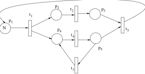
1 t1 p2 p4 t2 t4 t3 p5 p3 t5 p N
Figure 2.14 Petri net for Forkjoin Model
The forkjoin Petri net model is shown in Figure 2.14. It shows the forking of one main thread to create other threads that execute in parallel and then finally the joining of these forked threads back to the main thread. This Petri net shows a very common model of con-current execution where the main process creates parallel executing sub-processes and waits for them to be finished before resuming execution.
The Forkjoin Petri net consists of 5 places(p1, p2,p3, p4 and p5) and 5 transitions(t1, t2, t3,t4 and t5). Each place has a bound of N. The initial state of this Petri net hasN tokens
in place p1 which represents the main thread and 0 tokens at all other places. Transition t1
forks the main thread p1 to sub-threads and transition t5 joins the sub-threads back to the
main threadp1. Thus, afork is a transition with more than one output places and ajoin is a
transition with more than one input places. Figure 2.15 also shows the reachability set of this net withN = 1.
10000
01010
00110 01001
00101
This section explains how the transition relation and reachability set for a Petri net model PN = (P,T,W,H,M0) are built using the initial marking and the Petri net structure.
Algorithm 2.16 shows how enabling relation for a transition t is built. Enabling relation fortrepresents the possible current states in which tis enabled. It is built using the enabling expression fort. Hence, enabling relation is the relation for expression∀p∈ P :m(p)≥ W(p, t)
∧m(p)<H(p, t) Relation enablingRelation(transitiont) 1: V := M × M; 2: for all p∈P do 3: R :={(m, m0)∈ M × M: m(p)≥W(p, t)}; 4: V := V ∩R; 5: R :={(m, m0)∈ M × M: m(p)< H(p, t)}; 6: V := V ∩R; 7: end for 8: return(V);
Figure 2.16 Building enabling relation
Similarly, Algorithm 2.17 shows how firing relation for a transition is built. Firing rela-tion for t represents the possible next reachable states when t is fired. It is built using the firing expression for t. Hence, firing relation is the relation for expression ∀p ∈ P :m0(p) = m(p) +W(t, p)− W(p, t).
Relation firingRelation(transitiont) 1: V := Relation forM × M; 2: for all p∈P do 3: R:={(m, m0)∈ M×M: m0(p) =m(p)+W(t, p)−W(p, t)}; 4: V := V ∩R; 5: end for 6: return(V);
Figure 2.17 Building firing relation
Taking the intersection of the two relations(enabling and firing) produces the transition relation for t. Algorithm 2.18 shows how the complete transition relation is built by taking the union of the relations for all transitions(built using Algorithms 2.16 and 2.17).
Relation buildTransitionRelation() 1: Q:= ∅; 2: for allt∈T do 3: F := enablingRelation(t) ∩ firingRelation(t); 4: Q:= Q∪F; 5: end for 6: return(Q);
Figure 2.18 Building overall Transition relation
Algorithm 2.19 shows how the Reachability set is built using the initial DD and Transition relation(obtained from Algorithm 2.18). The reachabilitySet DD initially consists of the ini-tial marking. Next the post image operator is applied on the reachabilitySet to find the next reachable states denoted by postImage DD. Then, the union of postImage DD and reachabili-tySet is done. This process of finding the post image and its union with the reachabilireachabili-tySet is repeated until the post image operation does not create any new markings to be added to the reachability set.
0 1: R := M0; 2: P := ∅; 3: while P 6=R do 4: P :=R; 5: I := PostImageOperator(T,R); 6: R := R∪I; 7: end while 8: return(R);
Figure 2.19 Algorithm for building Reachability Decision Diagram
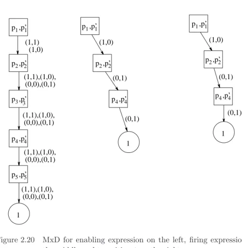
The Petri net in Figure 2.14 has 5 transitions. The enabling and firing expressions for transitiont1 are (m(p1)≥1) and (m0(p1) ==m(p1)−1∧ m0(p2) ==m(p2) + 1∧m0(p4) ==
m(p4) + 1). The enabling, firing and transition MxD fort1 are shown in Figure 2.20.
2.5 Model Checking
Model Checking [3, 11] is an automatic procedure for verifying a specification over a given model. This process involves three steps. Firstly, Kripke structures or finite automata are used to formally model a system. Secondly, the specification is written using either classical or temporal logic. Specification in this context means a propositional logic formula which could be a safety property like no deadlock or liveness. Lastly, it is verified if the model satisfies the specification or not. A model checker takes as input, a finite state model and a specification expressed as a temporal logic formula and returns either a true result or an execution show-ing why the specification is not satisfied by the model. Due to the size of the model(Kripke structure/finite automata), model checkers also suffer from the state explosion problem as they need to verify the specification amongst every execution of the model. Due to their compact structure, Reduced Ordered BDD’s are often used for representing the transition relation al-lowing verification of much larger models.
1, p ,p’2 p ,p’2 p ,p’4 1 (1,1), (0,0),(0,1) (1,1), (0,0),(0,1) (1,0), (1,1), (0,0),(0,1) (1,0), (1,1), (0,0),(0,1) (1,0), p ,p’4 4 1 (1,0) 1 p1,p’1 p1,p’1 2 p1 p ,p’2 2 1 ,p’ 4 (1,0) (0,1) (0,1) 2 (1,1) (1,0) p ,p’ p p ,p’ 3 3 4,p’4 5 5 (0,1) (1,0), (0,1)
Figure 2.20 MxD for enabling expression on the left, firing expression in the middle and transitiont on the right
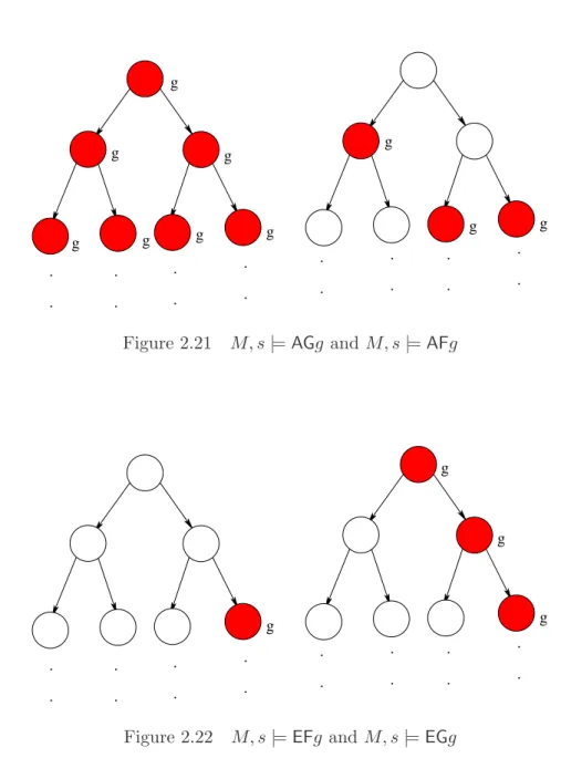
Temporal logic in contrast with the classical logic, allows reasoning about the system behavior over time.
• The temporal operatorGalso called the Global operator, along with a proposition logic formulap asGp, is true for a path ifpholds at all states(point of time) along the path.
• The future temporal operatorFwhen used with a propositional logic formulapasFp, is true for a path ifp holds at some state(points of time) along the path.
• The Until operator (pUq) is true for a path ifq holds at some state along the path, and p is true in all states before that state.
• The Next operator (Xp) is true for a path if p holds at the next state(points of time) along the path.
Computational Tree Logic also called CTL [6], is used to represent temporal logic. In CTL, a logical formula may consist of path quantifiers and temporal operators. Path quantifiers pro-vided by CTL are,A: for all paths andE: there exists a path.
A CTL formula can be a state or a path formula. M, s|=f, denotes the state formulaf holds in statesof model M. A state formula can be:
• An atomic proposition
• p ∧q,p ∨q,¬p, where pand q are state formulas
• A(g),E(g) where gis a path formula
A path formula can beXp,Fp,Gp,pUq, wherepand q are state formulas. The CTL operators can be reduced to the set (EX,EU,EG) using the following equivalence,
• AXp=¬EX¬p
• AFp=¬EG¬p
• EFp=EtrueUp
• AGp=¬EtrueU¬p
• ApUq =¬E[¬qU(¬q∧ ¬p)]∧ ¬EG¬q
Letp and q be propositional logic formulas, then
• EXp: This formula is satisfied by a state s if for some path from s, the formula Xp is satisfied.
• EpUq: This formula is satisfied by a statesif for some path froms, the formula (pUq) is satisfied.
• EGp: This formula is satisfied by a state s if for some path from s, the formula Gp is satisfied. . . . . . . . . . . g g g g g g g g g g . . . . . . Figure 2.21 M, s|=AGg and M, s|=AFg . . . . . . . . . . g g . . . . . . g g Figure 2.22 M, s|=EFgand M, s|=EGg
Algorithms to implement the three basic CTL operators are shown. Figure 2.23 shows the algorithm for implementing the CTL formulaEXp.
1: E := Satisfy(p); 2: T := Pre-Image(E); 3: return(T);
Figure 2.23 Algorithm for CTL formulaEXp
To implement the CTL formula EpUq as shown in Figure 2.24, initially the setY contains the set of states satisfying the logical formulaq. Then any state that satisfies the logical for-mulapand can reach a state that satisfiesEpUq, is added to the set until a fixed point is reached.
SetOfStatesEpUq(LogicFormulap, LogicFormulaq)
1: Y := Satisfy(q); 2: X := {}; 3: Z := Satisfy(p); 4: while Y 6=X do 5: X :=Y; 6: Y := Y ∪ (Pre-Image(Y) ∩Z); 7: end while 8: return(Y);
Figure 2.24 Algorithm for CTL formulaEpUq
The algorithm for implementing the formulaEGpis shown in Figure 2.25. The set of states satisfying EGp can be obtained by starting with the states satisfying the logical formulap. At each iteration, any state that cannot reach a state satisfyingEGpis removed from the set. This iterative process continues until a fixed point is reached.
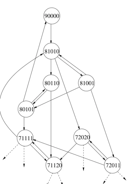
CTL model checking can be used to verify properties in systems modelled as Petri nets. It requires the generation of reachability graph, on which the model checking procedure is then applied. Figure 2.14 showed the Forkjoin Petri net model. Figure 2.26 shows the reachability graph of this petri net withN = 9.
SetOfStatesEGp(LogicFormulap) 1: Y := Satisfy(p); 2: X := {}; 3: while Y 6=X do 4: X :=Y; 5: Y := Y ∩ Pre-Image(Y); 6: end while 7: return(Y);
Figure 2.25 Algorithm for CTL formulaEGp
Let f = (p1 contains 8 tokens and p2 contains 1 token and p3 contains 0 tokens and p4 contains 1 token and p5 contains 0 token). Using CTL model checking, it is possible to check
if the CTL formula EX(f) is satisfied or not. It can be seen from the reachability graph that the markings/states which satisfy the logical formula f are {81010}. Next, the states which satisfy the formulaEX(f) form the set {90000}. As the initial state 90000 is included in this set, it is concluded that the given CTL formula is satisfied by the initial state. To evaluate the CTL formula EG(#p1 ≥8) where #p1 represents number of tokens inp1, all states satisfying
(#p1 ≥8) are found. The setY, satisfying (#p1 ≥ 8) is{90000,81010,80110,81001,80101}.
Initially, the set X satisfying formula EG(#p1 ≥ 8) is equal to set Y. Next, any state in Y that cannot reach a state inX needs to be removed. As every state inY can reach a state in X, a fixed point has been reached and{90000,81010,80110,81001,80101}is returned.
81010
90000
80110
81001
80101
72020
71120
71111
72011
CHAPTER 3. ENCODING SCHEMES
3.1 Overview
State encoding is a way to capture the state of a system. An encoding scheme basically maps the state of the system to decision diagram variable values. In case of Petri nets, captur-ing the state of the system would mean becaptur-ing able to capture the number of tokens at every place in the net at that time. Thus encoding a Petri net means encoding every place of the net using encoding variables. The size of the BDD can increase exponentially with increase in the number of encoding variables used to represent the Petri net model [16].
This Chapter explains the various encoding schemes and introduces a new encoding scheme called the k-hot encoding. Section 3.2 descibes the One-hot Encoding Scheme. Section 3.3 explains in detail the Logarithmic encoding. Native MDD encoding is explained in Section 3.4. Lastly, Section 3.5 introduces the new encoding scheme called k-hot encoding.
3.2 One-hot Encoding Scheme
Various encoding schemes have been proposed. The One-hot encoding scheme [15, 22] is extremely simple to implement. In an unsafe Petri net, ab-bounded place p uses b encoding variables under the One-hot scheme. Each of thesebvariables is used to encode the possibility of up tob tokens for that place. At most one of thesebvariables can be set at a time.
A marking m of a b-bounded Petri net with n places can be encoded using the One-hot scheme. Every placepof the Petri net, is encoded usingbencoding variables, thus in totaln·b
variable of place p. xp,i = 1, if m(p) =iwhere 1≤i≤b 0, otherwise (3.1)
To decode the marking at a placep(encoded usingbboolean variables),
m(p) =
i, if there exists an isuch thatxp,i = 1 where 1≤i≤b 0, otherwise
(3.2)
Thus under One-hot encoding, an ADD/MTMDD for the functionf =m(p) is equivalent to DD(ADD/MTMDD) for the variable xp,i where xp,i = 1. For safe Petri net models, this scheme uses the same number of encoding variables as the number of places in the safe Petri net. Thus this scheme is also known as one variable per place encoding scheme.
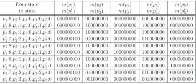
The Petri net in Figure 2.26 of Chapter 2 is aN-bounded Petri net. ForN = 9, each place in this net can have a maximum of 9 tokens. As per the One-hot encoding scheme, each of these five places use nine variables to encode the number of tokens present. Table 3.1 shows the encoding for placep1 of this Petri net. Thus the total number of encoding variables needed
xp1,1 xp1,2 xp1,3 xp1,4 xp1,5 xp1,6 xp1,7 xp1,8 xp1,9 m(p1) 0 0 0 0 0 0 0 0 0 0 1 0 0 0 0 0 0 0 0 1 0 1 0 0 0 0 0 0 0 2 0 0 1 0 0 0 0 0 0 3 0 0 0 1 0 0 0 0 0 4 0 0 0 0 1 0 0 0 0 5 0 0 0 0 0 1 0 0 0 6 0 0 0 0 0 0 1 0 0 7 0 0 0 0 0 0 0 1 0 8 0 0 0 0 0 0 0 0 1 9
Table 3.1 Encoding for place p1
As discussed in Chapter 2, transition function δ transforms a set of markings M1(also
called the from state) to a new set of markings M2(also called the to state) such that for every marking m2 ∈ M2, there exists a marking m1 ∈M1 such that m2 can be reached from
m1 on firing of a single transition which is enabled in m1. For example, the transition relation
transforms the marking [p1:9, p2:0, p3:0, p4:0, p5:0] to marking [p0
1:8, p02:1, p03:0, p04:1, p05:0].
The transition function of Petri Net in Figure 2.26 can be represented as a function over 90 variables (xp1,1,xp1,2, . . . ,xp5,9,x0
p1,1,x 0
p1,2, . . . ,x 0
p5,9), where the function evaluates to 1 if (x0
p1,1,x 0
p1,2, . . . ,x 0
p5,9) can be reached from (xp1,1,xp1,2, . . . , xp5,9) in one step. The enabling decision diagram of Algorithm 2.18 is is a graph over the 45 unprimed variables and the firing DD is a graph over the 45 primed variables. The reachability set of this Petri Net consists of 385 markings.
To encode the transition relation of a Petri net, both from and to states are encoded using the chosen encoding scheme. Section 2.4 of Chapter 2 showed how transition relation is built using the enabling and firing expressions of the net. The enabling and firing decision diagrams are built using one-hot encoding and hence the resulting transition relation is encoded as shown in Table 3.2. The unprimed variables encode the from state of the Petri net [p1:9, p2:0, p3:0,
p0 4:1, p05:0]. from state m(p1) m(p2) m(p3) m(p4) m(p5) to state m(p0 1) m(p02) m(p03) m(p04) m(p05) p1:9,p2:0,p3:0,p4:0,p5:0 000000001 000000000 000000000 000000000 000000000 p0 1:8,p02:1,p03:0,p04:1,p05:0 000000010 100000000 000000000 100000000 000000000 p1:8,p2:1,p3:0,p4:1,p5:0 000000010 100000000 000000000 100000000 000000000 p0 1:7,p02:2,p03:0,p04:2,p05:0 000000100 010000000 000000000 010000000 000000000 p1:8,p2:1,p3:0,p4:1,p5:0 000000010 100000000 000000000 100000000 000000000 p0 1:8,p02:0,p03:1,p04:1,p05:0 000000010 000000000 100000000 100000000 000000000 p1:8,p2:1,p3:0,p4:1,p5:0 000000010 100000000 000000000 100000000 000000000 p0 1:8,p02:1,p03:0,p04:0,p05:1 000000010 100000000 000000000 000000000 100000000 p1:7,p2:2,p3:0,p4:2,p5:0 000000100 010000000 000000000 010000000 000000000 p0 1:6,p02:3,p03:0,p04:3,p05:0 000001000 001000000 000000000 001000000 000000000 Table 3.2 Part of the transition relation for the Petri net shown in
Fig-ure 2.26 for N = 9
The efficiency of this scheme can be improved by interleaving the primed and unprimed variables. Instead of storing all unprimed variables of placep1followed by its primed variables,
an interleaved encoding stores xp1,1, the first unprimed variable for p1 followed by its corre-sponding prime variablex0
p1,1; then the second unprimed variable ofp1 which is xp1,2, followed by its primed variable x0
p1,2 and so on. This ordering usually produces a more compact BDD as compared to the normal ordering [20, 26].
3.3 Logarithmic encoding
The Logarithmic encoding [15, 22] scheme uses same or fewer encoding variables as com-pared to the One-hot. For an unsafe Petri net with up tobtokens at each place, the log-based scheme usesdlog(b+ 1)eencoding variables to encode the tokens at every place. xp,irepresents value of theith encoding variable of placep.
For a marking m, the value ofm(p) can be encoded as
xp,i=ai mod 2 (3.3)
wherea0 =m(p),ai=bai−1/2c and 0≤i≤ dlog(b+ 1)e −1.
The above encoding can be decoded to obtain the number of tokens at place p,
m(p) =
dlog(Xb+1)e−1 i=0
xp,i·2i (3.4)
In order to build ADD/MTMDD representing the functionf =m(p), the decison diagrams for constant 2i and variablex
p,i are built for alli, such that 0≤i≤ dlog(b+ 1)e −1. Next for all i, the multiplication operator is applied on DD’s for 2i and x
p,i. Addition of all such DD’s results in the graph representing functionf.
The Forkjoin Petri net model shown in Figure 2.26 withN = 9 can also be encoded under the Logarithmic encoding scheme where each of the five places of the Petri net use four variables to encode the number of tokens present. Thus under this scheme the total number of encoding variables required are 20 as opposed to the 45 variables required under the One-hot scheme. Place p1 can be encoded using four boolean variablesxp1,0, xp1,1,xp1,2 and xp1,3 as shown in Table 3.3.
As explained earlier, encoding the transition relation requires encoding both from and to states of the relation. With the log-based scheme, the from state will need four unprimed encoding variables and the to state will need four primed encoding variables. The encoded transition relation is shown in Table 3.4.
xp1,0 xp1,1 xp1,2 xp1,3 m(p1) 0 0 0 0 0 1 0 0 0 1 0 1 0 0 2 1 1 0 0 3 0 0 1 0 4 1 0 1 0 5 0 1 1 0 6 1 1 1 0 7 0 0 0 1 8 1 0 0 1 9
Table 3.3 Placep1 encoded using variables xp1,0,xp1,1,xp1,2 andxp1,3
Table 3.4 shows the transition from state [p1:9, p2:0, p3:0, p4:0, p5:0] to state [p0
1:8, p02:1,
p0
3:0, p04:1, p05:0] and from state [p1:8, p2:1, p3:0, p4:1, p5:0] to state [p01:7, p02:2, p03:0, p04:2, p05:0]
and so on. Interleaving the primed and unprimed variables can increase the efficiency of this encoding scheme as well.
3.4 Native MDD Encoding
Petri net models encoded using the native MDD encoding [15, 22], are represented using Multi Valued Decision Diagrams. The MDD encoding scheme uses a single encoding variable to encode the number of tokens present at a place in the Petri net. For ab-bounded Petri net model, the number of tokens at each place can be encoded using a single integer variable with value equal to the number of tokens at that place.
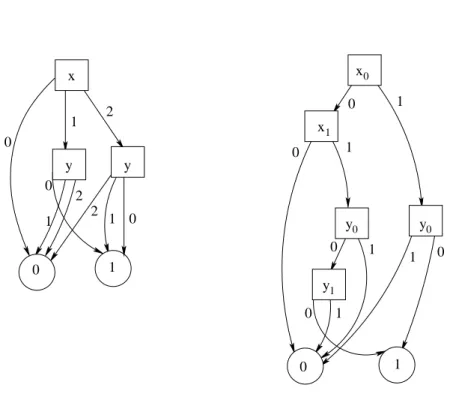
For a given BDD, its corresponding MDD can be built by groupinglBDD variables (binary variables) into a single MDD variable (multi-valued variable). The advantage of an MDD over its corresponding BDD is that, if the BDD requiresq memory accesses and the MDD requires zmemory accesses thenz≤q≤l·z[16]. Figure 3.1 shows a BDD and its corresponding MDD for the function:
from state m(p1) m(p2) m(p3) m(p4) m(p5) to state m(p01) m(p02) m(p03) m(p04) m(p05) p1:9,p2:0,p3:0,p4:0,p5 1001 0000 0000 0000 0000 p01:8,p02:1,p03:0,p04:1,p05 0001 1000 0000 1000 0000 p1:8,p2:1,p3:0,p4:1,p5 0001 1000 0000 1000 0000 p0 1:7,p02:2,p03:0,p04:2,p05 1110 0100 0000 0100 0000 p1:8,p2:1,p3:0,p4:1,p5 0001 1000 0000 1000 0000 p0 1:8,p02:0,p03:1,p04:1,p05 0001 0000 1000 1000 0000 p1:8,p2:1,p3:0,p4:1,p5 0001 1000 0000 1000 0000 p0 1:8,p02:1,p03:0,p04:0,p05 0001 1000 0000 0000 1000 p1:7,p2:2,p3:0,p4:2,p5 1110 0100 0000 0100 0000 p0 1:6,p02:3,p03:0,p04:3,p05 0110 1100 0000 1100 0000
Table 3.4 Part of the Transition relation of Petri net in Figure 2.26 with
N = 9
where 0≤x≤2 and 0≤y≤2. Note that the BDD uses 4 variables to represent the function as opposed to the 2 variables used by the corresponding MDD. Hence q ≤2z, where q and z are the memory accesses required by BDD and MDD of Figure 3.1.
In order to build an MTMDD representing the function f = m(p), a decision diagram having an edge from xp to terminal node m(p) is built. MDD encoding of a Petri net also involves encoding its initial state, transition relation and the reachability set. The initial state of the Petri net of Figure 2.26 with N = 9 is encoded as shown in Figure 3.2.
1 2 0 1 2 1 0 1 1 0 0 1 0 1 0 1 0 0 2 x0 1 0 0 1 y x y 1 0 1 0 x y y y
Figure 3.1 MDD forx > y on the left and the corresponding BDD on the right 9 0 0 0 0 p1 p2 3 p p4 p5 1
Figure 3.2 MDD representing the initial state of the Petri net shown in Figure 2.26 withN = 9
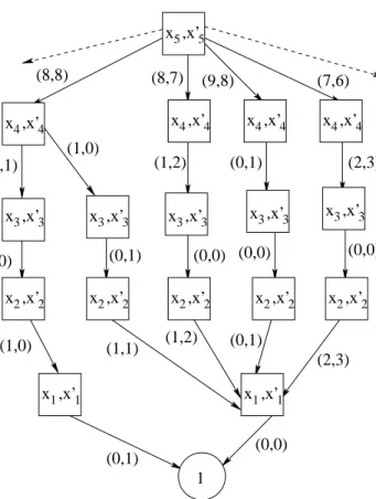
The transition relation of the Petri net of Figure 2.26 with N = 9 is encoded as shown in Figure 3.3. (8,8) (7,6) (0,0) (0,0) (0,1) (0,0) (0,1) (2,3) (0,0) (2,3) (8,7) (9,8) (1,2) (0,1) (1,0) (0,1) (1,1) (1,2) (1,1) (0,0) (1,0) 5 5 x ,x’ x ,x’4 4 x ,x’4 4 x ,x’4 4 x ,x’4 4 x ,x’3 3 x ,x’3 3 x ,x’3 3 x ,x’3 3 x ,x’3 3 x ,x’2 2 x ,x’2 2 x ,x’2 2 x ,x’2 2 x ,x’2 2 x ,x’1 1 x ,x’1 1 1
Figure 3.3 MxD representing a part of the transition relation of the PN shown in Figure 2.26 withN = 9
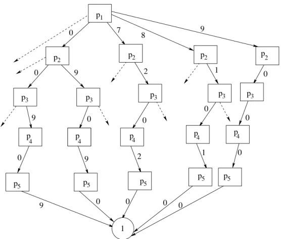
Figure 3.4. 0 0 9 0 9 9 0 9 7 2 0 2 0 8 1 0 1 0 9 0 0 0 0 0 p p p p p p p p 2 2 2 p2 5 5 5 5 5 p1 p3 p3 p3 p3 p3 p 4 p4 p4 p4 p4 1
Figure 3.4 MDD representing a part of the reachability set of the PN shown in Figure 2.26 withN = 9
3.5 Proposed Encoding Scheme - K-Hot Encoding
This thesis proposes a new encoding scheme called thek-hot encoding. The factork deter-mines the number of variables used by the encoding. The idea behind this encoding scheme is to not necessarily useb encoding variables to encodeb combinations(placepwith bound b). Ifb variables are used, it is easier as only one variable is set at a time and the position of the set-variable determines the value at that place.
With k-hot encoding we use fewer variables depending on the value ofk, and a maximum of kencoding variables can be set per place to represent a combination. Ifx variables are set for place(where x≤k), then the last x−1 variables must be set. A place p of the Petri net, with bound bis encoded using lvariables depending on the factor k.
l= & b k+ k−1 2 ' , where 1≤k≤l (3.6)
The values of k can be calculated for a fixed b such that ifk variables are used and all of them are set, it is enough to cover b.
b k +
k−1
2 ≥k (3.7)
The maximum value ofksuch that it covers bwhen all variables are set is l. Hence for k > l, the number of variables does not decrease with increase in k. Therefore, k-hot is equivalent to (k+1)-hot for k > l. The value of the ith variable of place p is represented as xp,i. For a markingm, the value ofm(p) can be encoded withl boolean variables using Algorithm 3.5.
The number of tokens at a place is determined by adding the value of the set tokens. The number of tokens at a place p, encoded usingl variables can be decoded as:
1: t:=m(p); 2: while l≥1do 3: if t≥lthen 4: xp,l:= 1; 5: t:=t−l; 6: l:=l−1; 7: else 8: xp,l:= 0; 9: l:=l−1; 10: end if 11: end while
Figure 3.5 Encoding place pusing k-hot encoding
In order to build ADD/MTMDD representing the function f = m(p), the decison diagrams for constant i and variable xp,i are built for all i, such that 1 < i < l. Next for all i, the multiplication operator is applied on DD’s for iand xp,i. Addition of all such DD’s results in the graph representing functionf.
2-hot encoding would require 5 variables to encode every place p in the Petri net of Fig-ure 2.26(N = 9). These boolean variables are xp,1, xp,2, xp,3,xp,4 and xp,5. A marking at p,
xp,1 xp,2 xp,3 xp,4 xp,5 m(p) 0 0 0 0 0 0 1 0 0 0 0 1 0 1 0 0 0 2 0 0 1 0 0 3 0 0 0 1 0 4 0 0 0 0 1 5 1 0 0 0 1 6 0 1 0 0 1 7 0 0 1 0 1 8 0 0 0 1 1 9
Table 3.5 Representing number of tokens at a place with bound 9 using 2-hot
Similarly, 3-hot encoding would require 4 variables to encode the place p.
xp,1 xp,2 xp,3 xp,4 m(p) 0 0 0 0 0 1 0 0 0 1 0 1 0 0 2 0 0 1 0 3 0 0 0 1 4 1 0 0 1 5 0 1 0 1 6 0 0 1 1 7 1 0 1 1 8 0 1 1 1 9
Table 3.6 Representing number of tokens at a place with bound 9 using 3-hot
An advantage of the k-hot scheme is the flexibility offered by this encoding. By setting different values of k, time and space metrics for computing the reachability set can be evalu-ated and compared. Interleaving the primed and unprimed variables can further improve the efficiency of this scheme.
The Forkjoin Petri net model introduced in Chapter 2 can be encoded using the k-hot encoding with different values of k. For k = 1, thek-hot encoding behaves exactly the same as the one-hot which was explained in Section 3.2. Hence, the following sub-sections explains the encoding of the Forkjoin model usingk= 2 and k= 3.
3.5.1 Encoding Forkjoin model with k as 2
Using Equation(3.5), we can calculate the number of variables required to encode each place of this model usingk-hot encoding with k as 2. Thus, we use 5 encoding variables per place in this case. The Transition relation for this Petri net is encoded as shown in Table 3.7.
from state m(p1) m(p2) m(p3) m(p4) m(p5) to state m0(p 1) m0(p2) m0(p3) m0(p4) m0(p5) p1:9,p2:0,p3:0,p4:0,p5 00011 00000 00000 00000 00000 p0 1:8,p02:1,p03:0,p04:1,p05 00101 10000 00000 10000 00000 p1:8,p2:1,p3:0,p4:1,p5 00101 10000 00000 10000 00000 p0 1:7,p02:2,p03:0,p04:2,p05 01001 01000 00000 01000 00000 p1:8,p2:1,p3:0,p4:1,p5 00101 10000 00000 10000 00000 p0 1:8,p02:0,p03:1,p04:1,p05 00101 00000 10000 10000 00000 p1:8,p2:1,p3:0,p4:1,p5 00101 10000 00000 10000 00000 p0 1:8,p02:1,p03:0,p04:0,p05 00101 10000 00000 00000 10000 p1:7,p2:2,p3:0,p4:2,p5 01001 01000 00000 01000 00000 p0 1:6,p02:3,p03:0,p04:3,p05 10001 00100 00000 00100 00000
Table 3.7 Part of the transition relation for Figure 2.26 withN = 9 using
k-hot encoding with kas 2
3.5.2 Encoding Forkjoin model with k as 3
Thek-hot encoding withkas 3, uses 4 variables to encode each place of the Petri net. Thus in all, 20 variables are used to encode the Initial state of this model. The encoded transition relation looks as follows:
from state m(p1) m(p2) m(p3) m(p4) m(p5) to state m0(p 1) m0(p2) m0(p3) m0(p4) m0(p5) p1:9,p2:0,p3:0,p4:0,p5 0111 0000 0000 0000 0000 p0 1:8,p02:1,p03:0,p04:1,p05 1011 1000 0000 1000 0000 p1:8,p2:1,p3:0,p4:1,p5 1011 1000 0000 1000 0000 p01:7,p02:2,p03:0,p04:2,p05 0011 0100 0000 0100 0000 p1:8,p2:1,p3:0,p4:1,p5 1011 1000 0000 1000 0000 p01:8,p02:0,p03:1,p04:1,p05 1011 0000 1000 1000 0000 p1:8,p2:1,p3:0,p4:1,p5 1011 1000 0000 1000 0000 p01:8,p02:1,p03:0,p04:0,p05 1011 1000 0000 0000 1000 p1:7,p2:2,p3:0,p4:2,p5 0011 0100 0000 0100 0000 p0 1:6,p02:3,p03:0,p04:3,p05 0101 0010 0000 0010 0000
Table 3.8 Part of the Transition relation for Figure 2.26 withN = 9 using

![Figure 2.9 BDD for ¬(x 1 ∧ x 3 ) on the left and x 2 ∧ x 3 on the right [4]](https://thumb-us.123doks.com/thumbv2/123dok_us/10219377.2925799/23.892.243.676.315.609/figure-bdd-x-x-left-x-x-right.webp)