MACHINE LEARNING FOR ANOMALY DETECTION IN OVERLAPPING AERIAL IMAGE STREAMS
A Thesis by
TRAVIS TAGHAVI
Submitted to the Office of Graduate and Professional Studies of Texas A&M University
in partial fulfillment of the requirements for the degree of MASTER OF SCIENCE
Chair of Committee, Jean-Francois Chamberland Co-Chair of Committee, Krishna Narayanan
Committee Members, Gregory Huff Dylan Shell Head of Department, Miroslav Begovic
August 2017
Major Subject: Electrical Engineering
ABSTRACT
This thesis work is an exploration into the application of machine learning to a cur-rent problem relating to streams of aerial images, with application to the imaging systems within the Texas A&M GEOSAT group and to the Texas A&M AgriLife Extension Ser-vice. The streams of images referred to are taken by a unmanned aerial vehicle (UAV) over some space of land.
Our problem relates to flight inconsistencies in the UAV. In an ideal scenario, our UAV captures a set of images from a specified height, pointed normally at the ground, with a predetermined amount of overlap between images. However, due to inconsistencies inherent in most flights, the UAV will occasionally tilt or swing in such a way that the images captured are not in line with adjacent images, i.e., they do not have the required amount of overlap, and their information may be blurred. This creates a problem when attempting image stitching afterwards, as such anomalous images will be irreconcilable with adjacent images. A prime goal then consists of designing a system which can, in pseudo-real-time, detect images which are out of line, through the use of feature extraction and machine learning, so that they can be discarded and possibly recaptured.
Our research compares and evaluates a number of image features and distance metrics, along with supervised classification learning algorithms, on the basis of their performance in this task. After feature evaluation, pixel intensity distribution, binary robust independent elementary features (BRIEF), and blob detection were selected as image features. The classification models chosen include logistic regression, neural networks, decision trees, and support vector machines (SVM).
After training and testing, the logistic regression model yields the highest performance, with a detection rate of 95.6% and a false alarm rate of 7.7%, making this a viable option
for this task. Neural networks and SVM yield lower levels of performance in detection and false alarm rates, respectively. Decision trees offer a very low detection rate of 11.9%, and are thus concluded to not be an ideal model for this task.
CONTRIBUTORS AND FUNDING SOURCES
Contributors
This work was supported by a thesis committee consisting of Professor Jean-Francois Chamberland (advisor), Professor Krishna Narayanan (co-advisor), and Professor Gregory Huff of the Department of Electrical and Computer Engineering and Professor Dylan Shell of the Department of Computer Science and Engineering.
The data analyzed for Chapter III was provided by the TAMU GEOSAT group. The analyses depicted in Chapter II were conducted in cooperation with Professor Jean-Francois Chamberland of the Department of Electrical and Computer Engineering.
All other work conducted for the thesis was completed by the student independently. Funding Sources
Graduate study was supported by a research assistantship from the TEES-AgriLife Center for Bioinformatics and Genomic Systems Engineering (CBGSE).
NOMENCLATURE
ANN Artificial Neural Network
BD Bhattacharyya Distance
BRIEF Binary Robust Independent Elementary Features
EMD Earth Movers Distance
MSE Mean Square Error
RGB Red, Green, Blue (color image representation)
SVM Support Vector Machines
UAS Unmanned Aerial System
TABLE OF CONTENTS
Page
ABSTRACT . . . ii
CONTRIBUTORS AND FUNDING SOURCES . . . iv
NOMENCLATURE . . . v
TABLE OF CONTENTS . . . vi
LIST OF FIGURES . . . viii
LIST OF TABLES . . . ix
1. INTRODUCTION . . . 1
1.1 Motivation . . . 1
1.2 Problem Setting and Formulation . . . 2
2. METHODOLOGY . . . 5
2.1 Data Preparation . . . 5
2.2 Image Feature Evaluation . . . 6
2.2.1 Distribution Distances . . . 6
2.2.2 Image Feature Descriptors . . . 8
2.2.3 Blob Detection . . . 10
2.2.4 Local Binary Patterns . . . 11
2.3 Learning Algorithms . . . 11
2.3.1 Logistic Regression . . . 12
2.3.2 Artificial Neural Networks . . . 12
2.3.3 Decision Trees . . . 14
2.3.4 Support Vector Machines . . . 15
2.4 Testing Methodology . . . 15
3. RESULTS . . . 17
3.1 Feature Evaluation . . . 17
3.1.1 Pixel Distribution . . . 17
3.1.3 Blob Detection . . . 18
3.2 Learning Algorithm Evaluation . . . 18
4. SUMMARY AND CONCLUSIONS . . . 23
4.1 Further Study . . . 24
LIST OF FIGURES
FIGURE Page
2.1 A general ANN . . . 14 3.1 Plot of MSEs between distributions of consecutive image pairs. . . 18 3.2 Plot of Earth mover’s distances between distributions of consecutive image
pairs. . . 19 3.3 Plot of Bhattacharyya distances between distributions of consecutive
im-age pairs. . . 20 3.4 Plot of BRIEF matches for consecutive image pairs. . . 21 3.5 Plot of the percentage of keypoints matched between consecutive image
pairs. . . 21 3.6 Plot of the difference in number of blobs between consecutive image pairs. 22 3.7 Plot of the difference in total blob area between consecutive image pairs. . 22
LIST OF TABLES
TABLE Page
1. INTRODUCTION
1.1 Motivation
In general, this thesis deals with the application of machine learning to detection and image segmentation tasks in the context of agricultural imagery. We consider the analysis of streams of images, taken aerially, as well as the structure of single images, based on spa-tial and spectral data. The streams of images are stitched together during post-processing to create large mosaicked maps of the monitored areas. Our first task involves ensuring that the stream of images meets the proper criteria for stitching while the images are being taken. Due to the large amount of data involved, feature extraction and machine learning are applied.
The broad motivation for this project is rooted in concerns that have an urgent global impact. As current global population estimates reach 7.5 billion, with simultaneous cli-mate change, there is a general scientific consensus that we are heading towards an im-pending water shortage. Already, while the supply of usable fresh water has been declin-ing, the overall demand for water has tripled since the 1950s. It is estimated that, by 2025, up to two thirds of the world’s population could be water-stressed [1]. In fact, numerical models that account for climate change, water needs, and socioeconomic variables show that not only is a large percentage of the world currently experiencing water shortage, but that demands for water are a greater factor than greenhouse warming when considering the state of water systems over the next several years.
A somewhat promising avenue for mitigating this problem is in the area of precision agriculture. Most estimates place the share of global water usage for irrigated agriculture at 70%, making it by far the dominant use of water [2]. It is predicted that greater overall yield potential will have to come from gains in net productivity of farming. Precision
agriculture has been shown to potentially increase farm profits by a significant amount with data collection, mapping of blackgrass weeds, and precision application of fertilizer, without even including precision irrigation [3].
Recent and continuing advances in technology and data science offer increased effi-ciency and productivity in many areas. Of particular application to agriculture are un-manned aircraft systems (UAS), commonly referred to as drones. UAS are simultaneously becoming lighter and gaining increased flight times and carrying capacities. This provides enhanced opportunity for developing automated systems for surveying and irrigating agri-cultural areas; a UAS equipped with GPS and imaging can map a plot of land, providing information on biomass, crop growth and quality, weed prevalence, etc. Research into increased efficiency and productivity of these systems is vital to the correlated increased net productivity of irrigated farming. As stated, we believe improvement to precision agri-culture has the potential to contribute to alleviation of the current and forecasted water scarcity.
1.2 Problem Setting and Formulation
To describe the setting of the problems addressed in this thesis, it is first necessary to mention that these problems are part of an overall project to develop a system for quality aerial agricultural imagery at Texas A&M University. In the current setting, members of AgriLife determine when and where to take the images, members of the Engineering College perform the flights, and members in the Electrical and Computer Engineering department are assisting data cleaning and analysis as well as pertinent system design. Once a flight time and location has been set, the UAV is flown at a height of 50 to 100 meters. Speed and image capture delay are adjusted to achieve approximately 75% overlap between consecutive images. Once the flight is complete, the image data is transferred to a member of the TAMU GEOSAT who, through specialized software, performs image
stitching to create one image of the area. The creation of a single, accurate mapping of the monitored area is the overall goal of the flight and imaging process. The map, which may be hyperspectral or multispectral, is then used for a variety of tasks related to precision agriculture.
It is the performance of this image stitching that we first address. For optimal per-formance in image stitching, both in terms of time taken and output quality, the camera should be pointed directly towards the ground and generate the desired amount of overlap between adjacent images. However, the limits of current technology mean that the imag-ing module on the UAV is not always pointed directly towards the ground when an image is taken. Turbulence, swinging, and swaying of the aircraft is likely to result in images that are not pointed directly at the ground, and hence may also not contain the desired amount of overlap. Such images will be referred to as anomalous, and can result in large increases in post-processing time, as well as sub-optimal output from mosaicking.
These anomalous images are difficult for the image stitching program to handle. In general, image stitching requires predictable overlap between images, as well as nearly identical regions of overlap, in order to locate unique features that can be matched to determine where overlap exists. With thousands of images, the process is very computa-tionally intensive to match all images and obtain a single map, even in an ideal scenario. In our case, anomalous images can be thought of as images that simply do not fit in with any other images. When the program attempts to feature-match these anomalous images with adjacent ones, the result is that the computation time is increased while the overall quality of the result is sacrificed.
The current system of addressing this problem is to have a human try to find these anomalous images by hand and remove them before processing. The first issue with this strategy is that this is a tiring and time-consuming process for the image reviewer, as well as the potential for human error in an otherwise mostly automated process. Secondly, if
the images are only removed afterwards, there is no chance to re-take the images, leaving the possibility for gaps in the final output if there are large regions of anomalous images. Our goal is to develop a system for detecting these anomalous images in pseudo-real-time, i.e., during the flight, so that they may be re-captured if necessary.
Algorithms do exist for explicitly finding the overlap between images, based on tak-ing convolutions and Fourier transforms. However, as stated previously, these are high-resolution images with many bands, and therefore contain a large amount of data. Addi-tionally, convolutions and Fourier transforms cannot be calculated in linear or sub-linear time. In our tests, the comparison of two images to find overlap took on the order of 100 seconds using a single CPU. Given that this does not allow for a stream of images to be processed in near-real time, our instinct is to extract features which can then be compared and processed to predict whether the desired level of overlap is present in the images. This process of operating on a set of extracted features rather than the entire volume of informa-tion is called feature extracinforma-tion and dimensionality reducinforma-tion. A key focus of this feature extraction/dimensionality reduction is the interplay between faster computing times and a loss of information. Ideally, features are extracted which preserve the information relevant to our task while, to some degree, discarding the unnecessary information. After this, the image features between each pair of consecutive images must be compared to create a feature vector. Each feature vector can then be associated with a label that states whether or not the pair of images contains acceptable overlap.
Beyond assessing the value of various image features, we evaluate a few different learning models for classifying the images as regular or anomalous. This setting, in which labeled feature vectors are used to train a model, is called supervised classification. The la-beled data is split between a training and testing set, which can be used to create predictive models as well as evaluate their performance.
2. METHODOLOGY
Our methodology for this research consists of several steps. First, the larger data archive is accessed; and the datasets, selected. Next, the data is cleaned, and labeled according to our criteria. Once the data is prepared, we perform feature evaluation: the process of extracting image features and analyzing them for their potential use in learning algorithms to detect anomalous images. Various distance metrics are then calculated, and again these metrics are analyzed for their utility in distinguishing acceptable images from anomalous ones. Finally, these metrics for each pair of consecutive images are concate-nated, along with the previously generated labels, and used as training data in our learning algorithms. Beyond this, various synthetic features are generated, and the parameters of the learning models are adjusted to achieve optimal results.
2.1 Data Preparation
To obtain usable datasets for training and testing, we first access the raw data. Once imaging flights run by the Texas A&M GEOSAT group are completed, the raw data is pushed to a network drive. The data is ordinarily then accessed by another member of the GEOSAT group, who performs orthomosaicking to produce a single map of the tar-get area. As stated in the problem formulation, this raw data generally contains images which are problematic, i.e., the camera was not pointed normally towards the ground, and thus the images are not reconcilable with respect to the surrounding images. Our goal in selecting data from the source is to find datasets over unique areas which are sufficiently large, generally more than 1000 usable images, and which have a sufficient percentage of anomalous images.
The data selection yielded four large datsets, totaling 8768 images. Since the current imaging process has the camera taking images before and during takeoff, as well as
dur-ing and after landdur-ing, these images have to be identified and removed. After this initial data cleaning, our datasets totaled 4863 images. The images are then searched through manually in order to create a list of anomalous image names which can later be used to generate label vectors for training and testing. After this process, 244 anomalous images were discovered among the four datasets, achieving a target rate of roughly 5%.
Finally, in accordance with most image processing standards, the images are all con-verted to grayscale. There are a few reasons for this: the first is that luminance (i.e., the grayscale values from a color image) is revealing enough for the vast majority of image processing task; a secondary reason is to ease processing time by cutting the data process-ing by 2/3, which is particularly important to our application.
2.2 Image Feature Evaluation
In this problem, we wish to find a set of features that can be quickly extracted from images, and used to train a model to identify images that do not belong in the stream. The first step in this process is to evaluate features to find ones that are suitable to our needs: quickly extracted and sufficiently distinguishing between overlapping and non-overlapping images.
Several types of image features are explored for this purpose. Pixel distributions, bi-nary features, local bibi-nary patterns, and blob detection were all extracted for a subset of the overall dataset and evaluated for their efficacy. Once image features are extracted, a few distance metrics are applied to compare the features between consecutive images. The distances are then compared between instances of acceptable pairs of images and pairs which contain anomalies to determine if the feature is usable.
2.2.1 Distribution Distances
When thinking of the differences between overlapping and non-overlapping images, pixel distribution was one of our first ideas. Pixel distribution is a very simple feature to
extract: it can be done in linear time with respect to the number of pixels, and is easily dis-tributable. Furthermore, it is clear that images with a large overlap will have fairly similar pixel distributions (since much of their content is nearly identical), and non-overlapping images may be dissimilar.
Once pixel distributions are extracted, a method for comparing the distributions is needed. From the field of statistics, there are a few methods for calculating “distances” between distributions: the higher the distance, the less similar the distributions are in some way.
The first distance metric we looked at is a very common method for calculating the distance between two sets of numbers: the mean-squared error or MSE. Essentially, the MSE is the L-2 norm of the errors or differences between the two sets of numbers. If we consider the vector p to be one distribution and the vector qto be another distribution, each of lengthn, then the MSE is given by:
1 n n X i=1 (pi −qi)2 ! . (2.1)
While the MSE does provide a distance between the two distributions, it is more suited to calculating errors, as the name suggests. Another distance metric, called the Bhat-tacharyya distance, is actually designed to measure the similarity between two continuous or discrete probability distributions. It is calculated by taking the negative of the log of the closely related Bhattacharyya coefficient. The Bhattacharyya coefficient was designed to be a metric for the amount of overlap between two distributions, defined as:
BC(p,q) = n X i=1 √ piqi. (2.2)
Making the Bhattacharyya distance equal to: BD(p,q) =−ln n X i=1 √ piqi ! . (2.3)
Another potential distance metric for distributions is the Earth Mover’s Distance (EMD), known in mathematics as the Wasserstein metric. If the distributions are considered to be two different ways of arranging piles of mass, then the EMD gives the minimum amount of mass that needs to be moved times the distance it is moved in order to turn one set of piles into another.
Formally, the EMD is defined as the solution to: min m P i=1 n P j=1 fi,jdi,j
Wherefi,j is the mass moved between biniandj in the two discrete distributions, and
di,j is the distance between binsi andj. This is subject to the constraint that the masses
moved transform one distribution into the other. This minimization can then be solved as a linear programming problem.
It is worth noting that the Bhattacharyya distance and MSE are calculated in linear time with respect to the number of possible intensity values, while the EMD is not. 2.2.2 Image Feature Descriptors
As stated, other features are needed in order to create a robust detection system. From the field of image processing, there are many image features that can be calculated quickly; our goal is to find features which can be compared and matched among consecutive images in a stream to determine if the images are overlapping by the desired amount. In image processing, keypoints are loosely defined as “interesting” parts of an image – locations in which there is a spike or trough or unique pattern relative to the rest of the image. The idea with these feature descriptors is to locate a set of keypoints in each image, create
descriptors for those points, and then attempt to match them between images to infer that the regions enclosed by matched descriptors are overlapping.
For our feature descriptor extraction, we use corner detection to determine the key-points used for the descriptors. An edge in an image is defined as a series of key-points along which the brightness in an image changes drastically. Generally, these are located by first finding points at which the brightness changes, and then locating connected components among these points. A corner, then, is a point at which two edges meet or at which there are two edge directions very close to a point in an image.
From previous research into image classification using feature descriptors [4], we iden-tified the SIFT feature as a potential feature which does incorporate spatial information. This is a scale-invariant feature transform (SIFT) which can be implemented in real time and easily matched between images using L-2 norm differences.
Further research revealed that the binary robust independent elementary features (BRIEF) would be better suited to our purposes. First, the BRIEF is calculated in less time than SIFT and performs similarly or better on benchmark tests[5]. Furthermore, the BRIEF keypoints can be matched between images using a simple Hamming distance, rather than the L-2 norm used for SIFT, which also aids in faster processing. Finally, although it is considered a disadvantage generally, BRIEF is not scale-invariant like SIFT. Since a scale change between images would not be expected or acceptable, scale-invariance would only result in false matches for our purposes, so the lack of scale-invariance is an advantage. The full derivation of BRIEF is both lengthy and irrelevant to our immediate research, so it is not included here. The BRIEF is obtained by first splitting the image into patches based on keypoints, and performing a set of pairwise intensity tests where the intensity of a smoothed patch is compared to another. The BRIEF then consists of a bitstring repre-senting the outcome of all pairwise tests between image patches.
outcome of intensity tests between the corresponding image patch and all other patches. As stated, matching keypoints between images can then be performed by calculating the Hamming distances between these substrings. A set of matches for each pair of consecu-tive images is generated, under the constraint that two matching keypoints cannot be more than 1/4 of the image size apart in their respective locations. This ensures that keypoints are not matched that violate the requirement of about 75% overlap in consecutive images. As a metric for comparing the BRIEFs of two images, we look at both the number of keypoints matched as well as the percentage of total keypoints matched. This is slightly different than the distance metrics calculated for other features in that a higher value in-dicates a higher probability that the images are acceptable, but nonetheless yields a single value comparing two images.
2.2.3 Blob Detection
Blob detection is the process of identifying regions in an image that differ from the surrounding regions. This is similar to the keypoints and descriptors described in the previous section, but involves a continuous group of pixels rather than the single points identified by keypoint or corner detection. More specifically, in our grayscale setting, blobs represent relatively bright or dark spots in an image.
Blobs can be easily calculated by first convolving the target image with the Gaussian kernel:
g(x, y, t) = 1 2πte
−x2+y2
2t .
Then, the Laplacian of this new image is generated, yielding strong positive values for dark spots and strong negative values for bright spots. The values are thresholded to detect blobs of a size relative to the size of the original Gaussian kernel. Multiple scales of kernels are used to detect blobs of varying sizes. The result for a single image is a set of blob locations and their corresponding radii.
To obtain a distance metric for two consecutive images, the blobs for both images are calculated. Then, we calculate the difference in number of blobs, as well as the difference in total blob area between the two images.
2.2.4 Local Binary Patterns
Local binary patterns are a method of classifying texture within an image. Texture, in image processing, refers to the relative smoothness or roughness of a section of an image. Local binary patterns are a relatively simple way of identifying the texture of a given pixel relative to its immediate neighbors. For a given pixel, a series of intensity tests are performed, the results of which form a binary string which can be converted to an integer. Then, a histogram is created based on the frequency of each of these integers in the image. While simple, local binary patterns and their histograms are used extensively in texture classification of images.
As a distance metric, we use the same distribution distance metrics as the general pixel intensity distributions. The evaluation of the LBPs and distances between acceptable and anomalous image pairs show that this metric is not suitable for classification. The values obtained are noisy and independent of whether the pair is anomalous or not.
2.3 Learning Algorithms
As stated in the problem formulation, we approach the problem with supervised binary classification in mind. Classification, as opposed to regression, associates a set of features with one of a number of labels, in the binary case there are only two of these labels. Supervised learning involves training a model with a set of features and their correct labels. The model then attempts to learn a set of parameters such that when the training data is passed through, the chosen cost function is minimized with respect to the correct labels. More generally, the model attempts to adjust its own parameters to output the correct labels for the training data. There are a large number of supervised classification algorithms
available and well-implemented in a number of languages. Our goal is to identify a number of these which are fundamentally different in their structure and observe the performance of these algorithms for our task.
2.3.1 Logistic Regression
The first among these is logistic regression: one of the most widely used classification algorithms. Logistic regression takes a labeled training set of feature vectors x(i) and corresponding binary labelsy(i). It then findsθto minimize the cost function:
J(θ) = 1 m m X i=1 1 2 hθ x (i) −y(i)2 (2.4)
wherehθ(·)is the logistic function defined ashθ(x) = 1+e−θT x1 .
Minimization of the cost function can be performed a number of ways, but the most common is through the gradient descent algorithm. Gradient descent works by altering the parameters in the direction of steepest descent at each iteration. For this, the gradient of the cost function relative to the parameters is taken, and the parameters are altered in the negative of this direction according to a predetermined step size. The step size or learning rate should be chosen so that the optimization converges as close as possible to the global minimum, while also considering that smaller step sizes take longer to converge. The learning rate can also be chosen adaptively at each step so that the steps become smaller as the minimum is approached.
2.3.2 Artificial Neural Networks
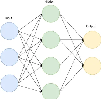
The next learning algorithm selected is the multi-layer perceptron (MLP) artificial neu-ral network (ANN). An ANN is a highly connected directed graphical model, in which the nodes are separated into layers. Each node in a given layer is connected directionally to each node in the following layer. In the first layer, called the input layer, the observation or
set of features is input into the nodes. From here, the information propagates from layer to layer according to the weights of the connections between nodes in each layer. A weighted linear summation is calculated using these weights, which is then passed to a non-linear activation function, such as the hyperbolic tangent function.
In training, the output at the final layer is compared to the desired output, and connec-tion weights are adjusted according to the error through a process called backpropagaconnec-tion. Starting at the output node, the error is calculated for the training set, and using a gradient descent, similar to that in logistic regression, the weight can be adjusted according to a learning rate and the error times the derivative of the non-linear activation function. For the hidden layers preceding the output nodes, a similar process is performed by propa-gating the error at the output layer back to the preceding layer, essentially evaluating the contribution of each node in this layer to the output error. A gradient descent is then per-formed in order to update the weights in this layer, followed by propagating these errors back to the preceding layer. This process is repeated until all hidden layers have been up-dated, at which point another iteration of the whole process is performed until a minimum is achieved.
ANNs have massive potential for performing at tasks which are difficult to define or explicitly program, but often require a large amount of training data and time to become effective. Multi-layer perceptron networks have the advantage of being able to learn non-linear models, but suffer from a sensitivity to feature scaling and non-unique minima. As with other ANNs, MLPs may require a great deal of tuning of hyper-parameters such as the size and the number of layers.
Figure 2.1: A general ANN
2.3.3 Decision Trees
Another classification algorithm considered is the decision tree. A decision tree takes a labeled training set of feature vectorsx(i)and corresponding binary labelsy(i), and finds a set of ordered thresholds to compare the features to in order to classify the vector. The model is visualized as a binary tree in which one starts at the root node and propagates towards the leaf nodes, which contain classification labels. Each node in the tree represents a threshold or set of thresholds on a set of features, and the child node is selected based on the comparison of the given features to the thresholds.
These thresholds are calculated based on the training data and a simple greedy algo-rithm which attempts to minimize the Gini impurity of the following layer of nodes. The Gini impurity of a set of training examples in a node is a measure of how likely an element of that set is to be mislabeled. If a set of examples contains n classes, then consider fi
expressed asP
i6=kfifk.
Decision trees are likely the simplest classification algorithm explored in this research, but may perform well if the structure of the problem is simple as well. The decision tree provides a good point of comparison for the other chosen learning algorithms.
2.3.4 Support Vector Machines
Support vector machines (SVMs) are the final classification algorithm explored. An SVM model represents the feature vectors or examples as points in space, such that the points can be separated by a hyperplane to classify the examples as belonging to one cat-egory or another. If the examples are linearly separable, then a maximum margin hyper-plane is generated by finding two parallel hyper-hyper-planes with a maximum distance between them such that the examples are still separated, and taking the parallel hyperplane directly in between these two planes. In the non-linearly separable case, a hinge loss function is calculated as the sum of distances of incorrectly labeled examples to the hyperplane.
The optimal hyperplane is found by first parametrizing the hyperplane asf(x) =β0+ βTxsubject to|β
0+βTx|= 1whereβ is the scale, andβ0 is the bias. Then, the distance between each pointxand a given hyperplane can be calculated as f||(βx||), which can then be minimized by a number of methods.
2.4 Testing Methodology
The testing methodology for this problem has multiple steps. First, a subset of the dataset is chosen for testing and evaluating the individual features. All features and dis-tance metrics are calculated for the pairs of consecutive images in the feature testing sub-set. For each feature, the standard deviation of the resulting distance metrics is calculated to ensure that the feature provides a sufficient amount of information. Next, a graph of these distance metrics is compared to a plot of the labels of the feature testing subset. The visual comparison of these plots is utilized to determine whether the feature provides some
level of distinction between acceptable and anomalous image pairs.
Once the features have been evaluated, and a subset of the features and distance met-rics has been selected to use in the learning algorithms, all labeled feature vectors are concatenated. The data is then split into an 80% training set and a 20% testing set. Each selected learning algorithm is then iteratively trained, tested, and tuned. Synthetic features, or non-linear combinations of existing features are added and tested for their contribution to performance. Since most of the learning algorithms explored here operate in a linear fashion, the addition of non-linear combinations can provide a pseudo non-linearity to the algorithms that has the potential to increase performance drastically. Tuning each learning algorithm involves adjusting the hyper-parameters of the model in an attempt to achieve a higher detection rate or lower false-alarm rate. Depending on the algorithm, this may involve adjusting class weights, learning rate, iterations, number of layers, etc., which is detailed in the following results section.
Finally, the data is split randomly several times into training and testing sets through random resampling or bootstrapping, and the testing scores averaged to obtain a realistic score of performance for each algorithm given the datasets.
3. RESULTS
The results of this research are split into the testing of features and learning algorithms, as detailed in the preceding testing methodology.
3.1 Feature Evaluation
As stated previously, plots of the various distances metrics for features are plotted in order to evaluate whether a feature is sufficient. The average extraction time for each feature for a single image is also shown. These features were extracted using a single core of an Intel i5 processor with a maximum clock speed of 2.7 GHz. Shown below are the plots and average extraction time for pixel distribution, BRIEF descriptors, and blob detection.
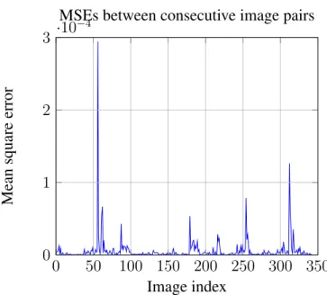
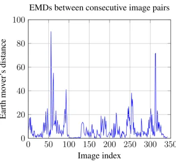
3.1.1 Pixel Distribution
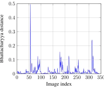
Below are figures showing the MSEs (figure 3.1), EMDs (figure 3.2), and Bhattacharyya (figure 3.3) distances between consecutive image pairs.
Spikes in the BD can be seen around the locations of the anomalous images, along with some spikes in other areas. The MSE has fewer and lower spikes around most anomalies, while the EMD is far noisier than other metrics. For this reason, the BD was chosen as the distance metric for pixel distribution. The average time for histogram calculation and Bhattacharyya distance calculation combined is 0.0473 seconds.
3.1.2 BRIEF Descriptors
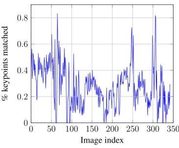
Below are figures showing the number of BRIEF matches between consecutive images (figure 3.4), as well as the percentage of keypoints matched between images (figure 3.5).
Contrary to the other metrics which are true distances, a dip can be seen in both metrics around the anomalous images. The average time for BRIEF extraction for a single image
0 50 100 150 200 250 300 350 0 1 2 3 ·10 −4 Image index Mean square error
MSEs between consecutive image pairs
Figure 3.1: Plot of MSEs between distributions of consecutive image pairs.
is 0.244 seconds. Distance metric calculation is a single operation of negligible processing time.
3.1.3 Blob Detection
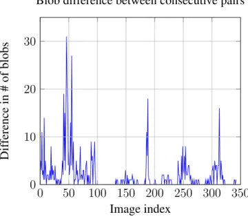
Below are figures showing the difference in number of blobs (figure 3.6) and the dif-ference in total blob area (figure 3.7) between consecutive image pairs.
Similarly to the distribution distance plots, spikes can be seen around the anomalous images, as well as in other places. The average time for extraction of blobs for a single image is 1.06 seconds – the longest time for any of the considered features.
3.2 Learning Algorithm Evaluation
To evaluate the learning algorithms, these distance metrics were concatenated into feature vectors, and fed along with the corresponding label vector to train each algorithm. As stated in the testing methodology, the models were then tuned to increase performance, and the final averaged values for detection rate, false alarm rate, and overall accuracy are
0 50 100 150 200 250 300 350 0 20 40 60 80 100 Image index Earth mo v er’ s distance
EMDs between consecutive image pairs
Figure 3.2: Plot of Earth mover’s distances between distributions of consecutive image pairs.
reported in table 3.1 below.
Algorithm Detection Rate False Alarm Rate Overall Accuracy
Logistic Regression 0.956 0.077 0.933
Decision Trees 0.119 0.033 0.899
Neural Network 0.75 0.038 0.959
SVM 0.924 0.258 0.743
Table 3.1: Performance of learning algorithms in anomalous image detection
The logistic regression model performed the best out of the four algorithms with a 95.6% detection rate and a 7.7% false positive rate. The decision tree predictably per-formed poorly, as it is a simple model incapable of considering the interaction between features. The SVM and neural network had decent performance, with the neural network missing 25% of anomalous image pairs, and the SVM having a fairly high false alarm rate
0 50 100 150 200 250 300 350 0 0.1 0.2 0.3 0.4 0.5 Image index Bhattacharyya distance
Bhattacharyya distance between consecutive image pairs
Figure 3.3: Plot of Bhattacharyya distances between distributions of consecutive image pairs.
0 50 100 150 200 250 300 350 0 10 20 30 Image index Number of matches
BRIEF matches between consecutive pairs
Figure 3.4: Plot of BRIEF matches for consecutive image pairs.
0 50 100 150 200 250 300 350 0 0.2 0.4 0.6 0.8 Image index % k eypoints matched
Percentage of keypoints matched between consecutive pairs
0 50 100 150 200 250 300 350 0 10 20 30 Image index Dif ference in # of blobs
Blob difference between consecutive pairs
Figure 3.6: Plot of the difference in number of blobs between consecutive image pairs.
0 50 100 150 200 250 300 350 0 1 2 3 ·10 4 Image index Dif ference in blob area
Blob area difference between consecutive pairs
4. SUMMARY AND CONCLUSIONS
The performance of the selected learning algorithms and features is promising. All of the selected features proved to be sufficiently discriminating, with the exception of the local binary patterns. This is understandable, as the feature may be too local to yield much information about the images as a whole. Furthermore, it is unclear that the texture would necessarily change when images are out of line, or that there could not be significant tex-ture changes in acceptable image pairs, e.g., the entrance of a body of water or a building. The most promising of the learning algorithms was the logistic regression model, which was able to detect 95.6% of anomalous images with a false-positive rate of 6.7%. The neural network had a very low false-positive rate of 3.8%, but failed to identify 1/4 of the anomalous images. As stated in the methodology section, neural networks typi-cally perform better with extremely large training sets, so there is potential for significant improvement with more training data. The SVM tuning (mainly of the soft margin hyper-parameter) was a balance between a high false-positive rate, and a relatively low detection rate. Since in our problem it is important to have as high of a detection rate as possible, we chose to increase this at the expense of also increasing the false-positive rate. The decision tree served its purpose as a point of comparison, but did not perform adequately in comparison to the other models. It is clear that this problem is not structured in a way that is amenable to tree learning.
With respect to the requirement to have the system run in pseudo real-time, the results are also acceptable, with room for improvement. All used features are able to be calculated on the order of one second or less, with the total feature vector calculation averaging 1.35 seconds utilizing processing power similar to that of the onboard data processing units. The imaging systems utilizing in capturing our training and testing data performed imaging
at a rate of 40-80 images per minute. The extraction of all features has the potential to be parallelized for performance increase. Since the model is not trained onboard the UAV, the model training time is not under any restrictions. Passing a new feature vector into any of the learning models amounts to a series of simple comparisons or matrix multiplications, the processing time of which is negligible.
Overall, the performance of the system, in particular the logistic regression model, indicates that machine learning is a viable option for the detection of anomalous images in aerial image streams. A small set of quickly extracted features, along with a model that is trained offline and ported to the onboard computer of a UAV is shown to have potential to alleviate the issue of unchecked anomalous images.
4.1 Further Study
Further study in this area could primarily involve the exploration of even more image features. As many aerial imaging systems involve multispectral or hyperspectral imagery, a third axis of data could provide opportunity for more revealing 3-dimensional features to be extracted. In particular, the segmentation of an image by spectral signature could identify differences between bio-matter which appear similar in grayscale. Beyond this, a full study into the design of a deep neural network trained with larger datasets could potentially yield an even more robust detection system.
Another direction of study would involve extending the classification of anomalies be-yond binary. Anomalies could be classified according to their nature (swinging in various directions, spinning, blur, etc.), or even quantified by how anomalous they are. This would lead to a multi-class detection system in the case of non-binary classes, and a regression problem in the case of quantified anomalies.
REFERENCES
[1] J. S. Charles J. Vörösmarty, Pamela Green, “Global water resources: Vulnerability from climate change and population growth,”Science, vol. 289, pp. 284–288, 2000. [2] K. Sentlinger, “Water scarcity and agriculture,” The Water Project, November
2016. Retrieved from https://thewaterproject.org/water-scarcity/water-scarcity-and-agriculture.
[3] T. A. Alex McBratney, Brett Whelan, “Future directions of precision agriculture,”
Precision Agriculture, vol. 6, pp. 7–23, February 2005.
[4] S.-S. C. Chein-I Chang, “Anomaly detection and classification for hyperspectral im-agery,” IEEE Transactions on Geoscience and Remote Sensing, vol. 40, pp. 1314– 1325, 2002.
[5] V. L. M. Calonder, “Brief: Binary robust independent elementary features,”Computer Vision-ECCV, pp. 778–792, 2010.