Forecasting volatility: does continuous time do better than discrete time?

Working Paper 11-25

Statistics and Econometrics Series 018

July 2011

Departamento de Estadística

Universidad Carlos III de Madrid

Calle Madrid, 126

28903 Getafe (Spain)

Fax (34) 91 624-98-49

FORECASTING VOLATILITY: DOES CONTINUOUS TIME DO BETTER

THAN DISCRETE TIME?

Carles Bretó** and Helena Veiga***

Abstract

________________________________________________________________

In this paper we compare the forecast performance of continuous and discrete-time

volatility models. In discrete time, we consider more than ten GARCH-type models and

an asymmetric autoregressive stochastic volatility model. In continuous-time, a

stochastic volatility model with mean reversion, volatility feedback and leverage. We

estimate each model by maximum likelihood and evaluate their ability to forecast the

two scales realized volatility, a nonparametric estimate of volatility based on

high-frequency data that minimizes the biases present in realized volatility caused by

microstructure errors. We find that volatility forecasts based on continuous-time models

may outperform those of GARCH-type discrete-time models so that, besides other

merits of continuous-time models, they may be used as a tool for generating reasonable

volatility forecasts. However, within the stochastic volatility family, we do not find such

evidence. We show that volatility feedback may have serious drawbacks in terms of

forecasting and that an asymmetric disturbance distribution (possibly with heavy tails)

might improve forecasting.

_______________________________________________________________________

Keywords:

Asymmetry; Continuous and discrete-time stochastic volatility models;

GARCH-type models; Maximum likelihood via iterated filtering; Particle filter;

Volatility forecasting.

* The authors acknowledge financial support from Financial Research Center/UNIDE,

from the Spanish Ministry of Education and Science, projects ECO2009-08100 and

MTM2010-17323 and Comunidad de Madrid research project CCG10-UAM/ESP-5494.

Helena Veiga also thanks George Tauchen and Tim Bollerslev for their helpful remarks

during her stay at Duke University; ** Departamento de Estadística and Instituto Flores

de Lemus, Universidad Carlos III de Madrid, Email:

[email protected]

; ***

Departamento de Estadística and Instituto Flores de Lemus, Universidad Carlos III de

Madrid. Financial Research Center/UNIDE, Avenida das Forças Armadas, 1600-083

Lisboa, Portugal. Email: [email protected]. Corresponding author.

Forecasting volatility: Does continuous time do better than

discrete time?

Carles Bret´o † Helena Veiga‡

July 26, 2011

Abstract

In this paper we compare the forecast performance of continuous and discrete-time volatility models. In discrete time, we consider more than ten GARCH-type models and an asymmetric autoregressive stochastic volatility model. In continuous-time, a stochas-tic volatility model with mean reversion, volatility feedback and leverage. We estimate each model by maximum likelihood and evaluate their ability to forecast the two scales realized volatility, a nonparametric estimate of volatility based on high-frequency data that minimizes the biases present in realized volatility caused by microstructure errors.

We find that volatility forecasts based on continuous-time models may outperform those of GARCH-type discrete-time models so that, besides other merits of continuous-time models, they may be used as a tool for generating reasonable volatility forecasts. However, within the stochastic volatility family, we do not find such evidence. We show that volatility feedback may have serious drawbacks in terms of forecasting and that an asymmetric disturbance distribution (possibly with heavy tails) might improve forecast-ing.

JEL-Classification: C10; C13; C53; C58; G17

Keywords: Asymmetry, Continuous and Discrete Time Stochastic Volatility Models, GARCH-type Models, Maximum Likelihood via Iterated Filtering, Particle Filter, Volatility Forecasting

∗

The authors acknowledge financial support from Financial Research Center/UNIDE, from the Spanish Ministry of Education and Science, research projects ECO2009-08100 and MTM2010-17323 and Comunidad de Madrid research project CCG10-UAM/ESP-5494. Helena Veiga also thanks George Tauchen and Tim Bollerslev for their helpful remarks during her stay at Duke University.

†

Departamento de Estad´ıstica and Instituto Flores de Lemus, Universidad Carlos III de Madrid, C/ Madrid 126, 28903 Getafe, Spain. Email: [email protected].

‡

Departamento de Estad´ıstica and Instituto Flores de Lemus, Universidad Carlos III de Madrid, C/ Madrid 126, 28903 Getafe, Spain. Financial Research Center/UNIDE, Avenida das For¸cas Armadas, 1600-083 Lisboa, Portugal. Email: [email protected]. Corresponding author.

1

Introduction

Forecasting volatility as accurately as possible is key to asset pricing, risk management and to efficiently manage investment portfolios. Hence, one can find in the literature many studies comparing different models in terms of their ability to forecast volatility (see for example Amin and Ng, 1997; Bluhm and Yu, 2002; Ederington and Guan, 2005, among others). However, forecast performance comparisons only seem to have considered discrete-time models, leaving aside continuous-time models. This is at odds with the extensive literature on continuous-time modeling, which goes back to the seminal papers by Merton (1969, 1971, 1973). Quoting Sun-daresan’s review of continuous-time methods in finance (Sundaresan, 2000):“continuous-time methods have proved to be the most attractive way to conduct research and gain economic intuition.”

In this paper we contribute to filling this gap between forecasting and volatility modeling by comparing the forecast performance of continuous and discrete-time volatility models using predictive ability tests. Johannes et al. (2009) is the only instance we are aware of that reports results on the forecast performance of continuous-time models, although it does not report any formal statistical test. But more importantly, we are not aware of previous work comparing continuous and discrete-time models in terms of their predictive ability.

This may in part be due to the fact that almost all continuous-time models considered in the literature are stochastic volatility models, i.e., they treat volatility as unobserved (but see Brockwell et al., 2006, for continuous-time GARCH-type models). In general, including unobserved components of this sort complicates inference, which becomes computationally expensive. In the comparison, we consider more than ten GARCH-type models in discrete-time, ranging from Gaussian GARCH to FIEGARCH with skew-t distributed disturbances. Due to the computational burden, we only include one stochastic volatility specification in continuous time and one in discrete time. In particular, we have chosen the well-known, discrete-time Asymmetric Autoregressive Stochastic Volatility (A-ARSV) model by Harvey and Shephard (1996); and the Log Linear One Variance Factor (LL1VF) stochastic volatility model in continuous time considered in Chernov et al. (2003). We have based the choice of the LL1VF model on the good results in terms of goodness of fit reported in Chernov et al. (2003) which considered a total of ten different continuous-time specifications (including affine, constant elasticity of variance and logarithmic models). We have chosen a one volatility factor model, instead of a larger number of factors, in order to make fair forecasting comparisons with the set of competitors. Moreover, the evidence regarding the inclusion of several volatility factors is not conclusive. Chernov et al. (2003) report that including more than one factor helps to capture the main empirical facts but Durham (2007) concludes that “a simple single-factor stochastic volatility model appears to be sufficient to capture most of the dynamics”.

We carry out an empirical predictive ability comparison of the models. We first estimate each model on a sample of daily stock data by maximum likelihood. For the GARCH-type models, we maximize the likelihood numerically. For the A-ARSV and LL1VF stochastic volatility models, we maximize the likelihood applying the iterated filtering algorithm pre-sented in Ionides et al. (2006), which we briefly describe in Section 2. To our knowledge, these are the first maximum likelihood fits reported for a continuous-time volatility model

and for the A-ARSV model.1 After the estimation step, we evaluate the volatility forecast accuracy for prediction of the Two Scales Realized Volatility (TSRV) introduced by Zhang et al. (2005). TSRV is a nonparametric estimator of volatility based on high-frequency data that minimizes the biases caused by microstructure errors. To obtain the TSRV for the out-of-sample evaluation, we used additional data consisting on intra-day 10-minute return observations. Although realized volatility has been already proposed as a candidate for mea-suring volatility forecast performance, we are not aware of any prior study using the more robust TSRV. We assess whether our results are unduly sensitive to a particular stock or to a performance measure by using data for three well-known international stocks: Coca-Cola, Disney and Microsoft; and by considering three performance measures: the mean squared error of forecasts; the mean absolute error of forecasts; and the proportion of the variability in TSRV explained by volatility forecasts (i.e., the R2 of a linear regression). Since these quantities are sample statistics, we perform the formal tests of conditional and unconditional predictive ability of Giacomini and White (2006). These tests have the advantage that they capture the effect of parameter uncertainty on the forecast performance and they can treat both nested and non-nested specifications in a unified framework.

In light of the predictive ability tests applied to our data, we conclude that volatility forecasts based on continuous-time models may perform better than GARCH-type discrete-time models. However, within the stochastic volatility family, we do not find such evidence. Since our search needed to be limited, more work restricted to stochastic volatility models needs to be done. These findings represent a valuable addition to the appeal and economic intuition of continuous-time models referred to at the beginning of this introduction. They also suggest directions in which to extend the LL1VF model, a task beyond the scope of this paper.

The rest of the paper is organized as follows: in Section 2, we introduce the continuous-time LL1VF stochastic volatility model and present parameter estimates for the three return series. In Section 3, we summarize how the target to forecast (the two scales realized volatility) is calculated and describe how we evaluate forecast performance. In Section 4, we introduce the set of alternative, discrete-time models and review the predictive ability tests which yield the empirical results discussed in Section 5. Finally, in Section 6, we conclude. To preserve the flow of the main themes of the paper, we defer to the Appendix additional derivations. Finally, figures and tables are gathered at the end of the paper.

1

Maximizing the likelihood for stochastic volatility models is not an easy task. Estimation of stochastic volatility models has instead been tackled with alternative approaches, including indirect inference (Gouri´eroux and Monfort, 1996), the efficient method of moments (Gallant and Tauchen, 1996), Bayesian methods (Jones, 2003) and simulated maximum likelihood (A¨ıt-Sahalia and Kimmel, 2007). See Broto and Ruiz (2004) and Ruiz and Veiga (2008) for detailed surveys on estimation methods for stochastic volatility models.

2

The continuous-time Log Linear One Volatility Factor

(LL1VF) model

As in Chernov et al. (2003), letP(t) be a share price quote of one company at instant t and reserve the notation U1(t) for the logarithm of P(t). Assume that the instantaneous return

of the asset at instantt,dP(t)/P(t), is approximated bydU1, which is in turn given by

dU1(t) = α10dt+ exp(β10+β12U2(t))(ψ11dW1(t) +ψ12dW2(t))

dU2(t) = α22U2(t)dt+ (1 +β22U2(t))dW2(t).

(1) In the first equation of model (1), α10 denotes the instantaneous expected return; σ(t) =

exp(β10 +β12U2(t)) is the instantaneous standard deviation (or instantaneous volatility),

in which β10 determines the long-run mean and β12 modulates the effect of the volatility

factor U2(t). Wi(t) with i= 1,2, are independent Wiener processes and the corresponding

ψ1i’s are correlation coefficients that satisfy the restrictionψ11 =

p

1−ψ₁₂2 . This restriction guarantees thatσ(t) is indeed the infinitesimal standard deviation ofU1(t). As a consequence,

the instantaneous correlation between returns and changes in variance (the leverage effect) is given by

corr(dU1(t), β12dU2(t)) =ψ12. (2)

The volatility factorU2(t) is modeled as an Ornstein-Uhlenbeck process. Its drift allows for

mean reversion ifα22 is negative andγ2= log(2)_α22 is the volatility half-live. A small value ofγ2

means that the volatility factor is persistent and shocks to volatility take time to dissipate. In this case, the volatility factor is said to be slow mean reverting.

The termβ22U2(t) allows the volatility of the volatility factor to be high when the factor

itself is high and is known as volatility feedback. As pointed out in Chernov et al. (2003), including this volatility feedback introduces a lower bound on the volatility factor. Heuristi-cally, the infinitesimal standard deviation of the volatility factor must satisfy 0≤1+β22U2(t),

from where −1/β22≤U2(t) follows. This lower bound on the volatility factor in turn implies

a positive lower bound on the infinitesimal volatility of the returns, i.e., expβ10−β_β12₂₂

. As we will show, this bound has serious implications. The lower bound implied by point esti-mates based on a given sample may change drastically if new observations are included in the estimation, limiting severely the forecast performance of the initial estimates. In spite of this lower bound, the inclusion of volatility feedback into the models can be justified by the in-crease in the estimation accuracy of the relationship between market volatility and the equity premium (see Yang, 2011, for a very recent study on volatility feedback and risk premium in GARCH models).

2.1 Parameter estimation

We estimate the LL1VF model using the iterated filtering algorithm of Ionides et al. (2006). The algorithm is based on a sequence of filtering operations which have been shown to converge to a maximum likelihood parameter estimate for general non-linear, non-Gaussian, partially-observed state-space models. The algorithm has successfully been implemented in different

applications (Ionides et al., 2006; King et al., 2008; Bret´o et al., 2009; He et al., 2010; Ionides et al., 2011). The first step of the algorithm consists on extending the model by letting fixed parameters become time-varying random walks. In these extended models, it is possible to filter these time-varying parameters using, for example, a particle filter. Particle filters are a flexible and effective tool based on sequential Monte Carlo (see Doucet et al., 2001, for a book-length treatment). These filtered estimates are interpreted as local estimates of the fixed “global” parameters of interest and averaged using their precision (or inverse uncertainty) as weights. Starting from some initial parameter estimates, this procedure is iterated reducing the variance of the random walks at each iteration. Eventually, the filtered local estimates are basically constant over time and, in the limit, the maximum likelihood estimates are achieved. The appropriate choice of algorithmic parameters is key for achieving the maximum of the likelihood.

We implement the iterated filtering algorithm using the software package POMP (King et al., 2010) written for the R statistical computing environment (R Development Core Team, 2010). In the particle filter used in the algorithm, we have used 4,000 particles and estimation runs typically involved 35 iterations with an exponentially cooling schedule with parameter 0.925. In order to filter efficiently, we derived an analytic expression for the distribution of the discretely sampled returnsU1n. Let

U1n = U1(n∆)−U1((n−1) ∆) σ_n2 = n∆ Z (n−1)∆ σ2(u)du. (3)

forn ≥1 and ∆ a time interval of interest (one day for the case of our daily data). Then, the LL1VF model implies a state-space model where the distribution of the measurements, conditionally on the unobserved state processesσ(t) andW2(t), is given by

U1n ∼ N   E=α10∆ +ψ12 n∆ Z (n−1)∆ σ(t)dW2t, V = 1−ψ122 σ_n2   . 2.2 Estimation results

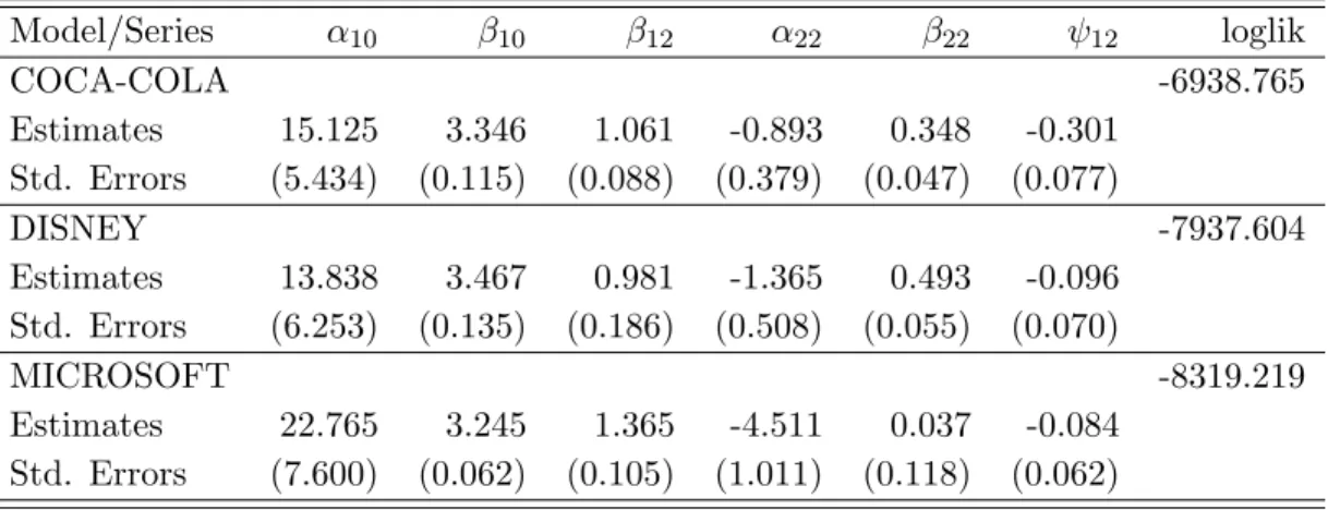
Table 4 reports point estimates and asymptotic standard errors for the three datasets. The estimation sample is from January 2, 1991 to January 22, 2007 (4046 daily observations) and is used to estimate all models considered in this paper. All data are adjusted for outliers.2 All estimates are in an annual scale since the time unit used in the estimation were years with trading days of length ₂₅₂1 years. We use an Euler-Maruyama discretization scheme with twenty four steps per trading day. The standard errors are obtained by inverting a Monte

2

We replace observations larger than seven standard deviations by their standard deviations estimated using a GARCH(1,1) model, taking into account the sign of the observations. This is particular important for the GARCH-type models since the parameter estimates are known to be affected by outliers (see Carnero et al., 2007).

Carlo approximation to Fisher’s information matrix (see Ionides et al., 2006). These standard errors give a reasonable idea of the scale of uncertainty, rather than being a tool for testing significance of the parameters. Confidence intervals based on profile likelihoods, much more computationally expensive, are preferable for drawing such inferences.

Most parameters seem to be estimated with precision, since the standard errors are in general an order of magnitude smaller than the point estimates. Coca-Cola and Disney present very similar point estimates, at least after taking into account the approximated standard errors. The only discrepancy is in the leverage effect which is estimated to be of larger magnitude (−0.301) for Coca-Cola than for Disney (−0.096) and for Microsoft (−0.084). Microsoft also differs from Coca-Cola and Disney in the volatility persistence. The estimate of mean reversion is ˆα22=−4.511, which implies that shocks to volatility are less persistent

than those that impact the other two series since the value of this estimate is around −1 for both series. Volatility feedbacks seem to be statistical significant for Coca-Cola and Disney. There are also some differences in what is inferred about the way the unobserved volatility factor affects return variability. In particular, smaller estimated baseline volatilities ( ˆβ10)

seem to be compensated by larger impacts of the volatility factor ( ˆβ12). The estimated

lower bounds of the volatility factor [−_ˆ1

β22,

∞] are −2.874, −2.028 and −27.027 for the Coca-Cola, Disney and Microsoft return series, respectively. These imply estimated volatility lower boundsexp ˆ β10− ˆ β12 ˆ β22 of 1.346, 4.380, and 2.440×10−15.

Regarding previous results based on the same family of models, Chernov et al. (2003) finds similar estimates for the mean reversion parameters and volatility feedback of the Dow Jones return series. However, our estimates of leverage for the three series are slightly lower (in absolute value) than those in Chernov et al. (2003), which may be explained by different periods being analyzed.

3

Evaluating Volatility Forecast Performance

The vast majority of the existing literature on volatility forecast performance measures the ability of a model to forecast the observed squared returns. In this paper, we differ from this approach by measuring the ability of models to forecast the Two Scales Realized Volatility (TSRV), which is a non-parametric estimator of the volatility obtained from an extended data set. We are aware of some attempts of assessing forecast performance by considering Realized Volatility (RV), defined as the sum of intra-day squared returns, as an alternative to squared returns (Andersen and Bollerslev, 1998). Nevertheless, this is to our knowledge the first volatility forecast evaluation corrected for the notorious effects of market microstructure. We describe this in detail below. Note that the volatility, and not the squared returns, is the information needed for efficient asset pricing, risk management and portfolio optimization.

3.1 Two Scales Realized Volatility

RV is only a consistent estimator of the true volatility when prices are observed continuously and without measurement errors (see Merton, 1980). Unfortunately, these ideal conditions are not met in general and RV is often biased due to market microstructure noises. Moreover, its

bias tends to get worse as the sampling frequency of intra-day returns increases, (see Andreou and Ghysels, 2002; Bai et al., 2004; Oomen, 2002). One way to minimize these biases is to use kernel-based estimators (see Barndorff-Nielsen and Shephard, 2004; Hansen and Lunde, 2005, 2006; Zhou, 1996) or sub-sample based estimators (see Zhou, 1996; Zhang et al., 2005). In this paper, we use the TSRV estimator by Zhang et al. (2005). Our choice is justified by A¨ıt-Sahalia and Mancini (2008), which report evidence that TSRV largely outperforms RV in terms of bias, variance and out-of-sample forecasting ability. Define the discretely observed return process as:

Yt=Xt+ut, (4)

whereXtis a latent true return process evolving in continuous time andutis an independent

disturbance around the true return that captures market microstructure effects. Since in high frequency financial asset returns are subject to frictions, it is wise to consider that the logarithm of the price is observed with error. Moreover, define

hX, Xi_T =

Z T

0

σ_t2dt, (5)

as the integrated variance over the interval [0, T] that may correspond to, for instance, a day. The integrated volatility, also known as quadratic variation, is then given by

[Y, Y]_T ≈ hL X, XiT + 2nE u2+ 4nE[u4] +2T n Z T 0 σ_t4dt 0.5 Z, (6)

where≈L denotes stable convergence in law, Z is a standard normal variable (see A¨ıt-Sahalia and Mancini, 2008) and nis the total number of observations. The bias due to the noise is 2nEu2, which is of the order O(n).

Zhang et al. (2005) propose an estimator of the quadratic variation that consistently estimates the bias due to the error. It consists on averaging the estimators obtained from sub-samples created by splitting the original grid of observation times, G = t0, ..., tn, into

sub-samplesG(k) fork= 1, ..., K. For instance, forG(1) we may start at the first observation and take an observation every 10 minutes, for G(2), we start at the second observation and take an observation every 10 minutes, etc. With this procedure, they construct an estimator with smaller variation, denoted [Y, Y](_Tavg) = _K1 PK

k=1[Y, Y]

(k)

T , that is obtained by averaging

the estimators [Y, Y](_Tk) obtained on the K grids. The K grids are of average size −n=n/K, wheren/K→ ∞asn→ ∞. Then, the TSRV is the bias-adjusted estimator for the quadratic variationhX, X[i_T built as

hX, X[i(_Ttsrv)= [Y, Y](_Tavg)− − n

n[Y, Y]T . (7)

The second term of the right hand side is the consistent estimator for the bias.

In this paper, we use intra-day 10-minutes return observations summing up 38 daily observations for each series.3 Figure 2 graphs this high-frequency measure of integrated volatility for all series for the out-of-sample period used in the forecasting evaluation (January 7, 2005 till January 22, 2007).

3.2 Evaluation Procedure

In order to evaluate the ability of a model specification to predict TSRV one-step ahead, we consider three performance measures: (i) mean squared error (MSE); (ii) mean absolute error (MAE); and (iii) the proportion of the TSRV variability explained by the forecasts (i.e., the R2 of a linear regression with a constant term). The last measure is based on Mincer-Zarnowitz volatility regressions in which the dependent variable is the TRSV instead of the squared returns. The latter is often a noisy proxy of the true volatility (see Andersen et al., 2005).

As proposed, for example, by Andersen and Bollerslev (1998) and Andersen et al. (2003), for (iii) we estimate by OLS the regression of a transformation of the TSRV on the forecasts for the same transformation of the volatility,

p

T SRVt+1 =β0+β1·σt+1|model+ut+1 (8)

and

ln(T SRVt+1) =β0+β1·ln(σ2)t+1|model+wt+1. (9)

Then, we calculate the R2 of regressions (8) and (9). We denote by MSE the mean squared error of the forecasts for σ and by MSE(∗) those for ln(σ2). MAE and MAE(∗) are defined analogously.

For the LL1VF model, we propose using the one-step ahead prediction mean of these transformations of the variance, i.e., fort∈ {0,1, . . .}:

σ_t+1|LL1V F =E _q σ2 t+1 U1,1:t and ln (σ2)t+1|LL1V F =E h ln (σ2_t+1) U1,1:t i

where σ_t2₊₁ is defined in equation (3). We could also use other summaries of the center of the prediction distribution (median, mode, etc.) but the prediction mean has the well-known property that, under the true model, it minimizes the MSE. Monte Carlo approximations to these prediction means were obtained using particle filters with 50,000 particles. This number of particles ensures that the values of the results for the MSE and MAE reported in Tables (6)-(8), which include Monte Carlo error, can be reproduced up to the second decimal. We implement the same evaluation procedure when considering filtering instead of fore-casting in Table (9), where we use filtering means, like Ehpσ2

t U1,1:t i , instead of one-step ahead prediction means.

4

Comparing Volatility Forecast Performance

In this section we formally define the set of discrete-time models to which we compare the predictive ability of the continuous-time LL1VF model. But first, we describe the statistical test which provides us with the empirical results of next section. We could directly compare the sample MSE and the rest of sample performance measures described above. However, such

a comparison would not take into account that these are sample statistics with an associated sampling variability. To be able to assign (approximate) confidence and significance levels to our results, we perform the conditional and the unconditional ability tests of Giacomini and White (2006) to compare the predictive ability of two alternative modelsgand f.

The tests consist on considering a forecasting horizonh and a given loss function L. The null hypotheses of the tests, in our particular case, are that the expected loss functions are equal: H0:ELt+h σt+h|model f −Lt+h σt+h|model g |Gt =E[∆Lt+h(σt+h)|Gt] = 0 H0:E Lt+h ln(σ2)t+h|model f −Lt+h ln(σ2)t+h|model g |Gt =E ∆Lt+h ln(σ2)t+h |Gt = 0, almost surely. LettingFt denote the time-t information set, the conditional test corresponds

toGt=Ft and Gt={∅,Ω} (the trivialσ-field) corresponds to the unconditional test.

To implement the one-step ahead tests, we conduct an artificial regression of ∆Lt+1 on

a 1× q vector λt, denoted “test function” (see Stinchcombe and White, 1998, for more

details). The test statistic is n×R2, where n and R2 are the number of observations and the uncentered R2 of this artificial regression. This statistic follows aχ2_q distribution with q

degrees of freedom.

For the conditional test, we follow Giacomini and White (2006) and use the 1×2 vector

λt= (1,∆Lt) as test function. Rejection of the null hypothesis indicates that the test function

has predictive power for the loss differences ∆Lt+1in the out-of-sample period. Once the null

is rejected, we establish a decision rule again following Giacomini and White (2006). Let ˆβ

denote the coefficient vector obtained by regressing ∆Lt+1 on λt. At time t, we choose the

t+ 1 predictions from model gif λ0_tβ >ˆ 0; and those from modelf if λ0_tβ <ˆ 0. Moreover, for the out-of-sample period oft1, . . . , T −1, we calculate the proportion of times the decision

rule chooses modelg. For this purpose, we build an indicatorS=n−1PT−1 t=t1I(λ

0

tβ >ˆ 0). The

rejection of the null hypothesis of the conditional test leads us to conclude that it is possible to predict which forecasting method will be more accurate in the future conditionally on the current information.

For the unconditional test, we choose the scalar test function to be equal to a constant, in particular λt = 1. The rejection of the null of the unconditional test leads us to conclude

that one of the forecasting methods is more accurate on average.

4.1 Discrete Time Models

Choosing which models to consider in our analysis is not an easy task. We include a good number of models for which we have found evidence that they outperform other specifications according to some loss function. In the context of conditional heteroscedasticity, we consider: the GARCH, the EGARCH, the hyperbolic GARCH (HYGARCH), the FIEGARCH, and the FIGARCH model with errors following Gaussian, t-Student and skew-t distributions. In the context of stochastic volatility, we consider an asymmetric autoregressive stochastic volatility (A-ARSV) model with Gaussian errors in discrete time (see Harvey and Shephard, 1996).

Stochastic volatility models clearly dominate other specifications when the objective is to calculate value-at-risk (see Gran´e and Veiga, 2008). Among others, Andersen and Bollerslev (1998), Hansen and Lunde (2005), Pagan and Schwert (1990), and West and Cho (1995) also

provide evidence that GARCH-type models yield accurate volatility forecasts. Additionally, Davidson (2004) reports encouraging empirical results for the HYGARCH with respect to Asian exchange rates and Koopman et al. (2005) shows that long memory4 models provide the most accurate forecasts of the Standard & Poor’s 100.

4.1.1 Asymmetric autoregressive stochastic volatility model (A-ARSV)

Formally, let the return of a financial asset at timet,yt, satisfy

yt = µ+σtt (10)

σ2_t = σ2_∗exp (ht) (11)

ht+1 = φht+ηt (12)

Here, µ and σ_t2 are the conditional expected value and variance of yt, σ∗ denotes a scale

parameter andht is an unobservable latent variable that is stationary for|φ|<1. Moreover,

(t, ηt)0 follows the bivariate normal distribution

t ηt ! ∼ N ID 0 0 ! , 1 δση δση σ2η !! (13)

whereδ, the correlation between εt and ηt, induces correlation between returns and changes

in volatility (see Taylor, 1994; Harvey and Shephard, 1996).

As in Section 2, we estimate the model parameters using iterated filtering. The particle filter used in the implementation uses 600 particles and estimation runs typically involved 35 iterations with an exponential variance cooling schedule with parameter 0.925. In order to implement the algorithm, we re-write the model as a state-space model with measurements following, conditionally on the unobserved variables σtand ηt, the distribution5

yt ∼ N E=µ+δσtηt, V = 1−δ2

σ_t2.

As for the LL1VF model, we propose using for the A-ARSV model the one-step ahead prediction mean: σt+1|A−ARSV =E _q σ2_t+1 h1:t 4

According to Parzen (1981), a stationary process {yt} with autocovariance γy is called a long memory process in the covariance sense if Pn

τ=−nγy(τ) → +∞ as n tends to +∞. Granger and Joyeux (1980)

provided a different definition of long memory. According to them, {yt} is a long memory process in the covariance sense with speed of convergence of order 2d, 0< d <1/2, wheneverγy(τ) =C(d)τ2d−1, asτ→ ∞

(here,C(d) is a function that depends ond).

5

Analogously to expression (1) for the LL1VF model, we consider modeling the correlation betweent and ηt by lettingtbe distributed as

p

1−δ2_ν

t+δηt

and ln (σ2)t+1|A−ARSV =E h ln (σ2_t+1) h1:t i ,

where σ2_t is defined in equation (12). We obtain Monte Carlo approximations to these pre-diction means using particle filters with 10,000 particles. Since discrete-time models are less demanding in terms of particles, this number of particles ensures that the results for the MSE and MAE reported in Tables 6-8, which contain Monte Carlo error, can be reproduced up to the second decimal. As for the LL1VF model, we implement the same evaluation procedure when considering filtering instead of forecasting, using Ehpσ2_t

h1:t

i

instead of the one-step ahead prediction mean.

4.1.2 GARCH-type models

Davidson (2004) proposes the HYGARCH model as an alternative to the FIGARCH since this model is able to generate long memory without behaving oddly whend, the parameter of fractional integration, approximates 1. Formally, let the prediction errorεt satisfy

yt−µ=εt=σtt, (14)

where σ_t2 is the conditional variance of εtgiven information at time t−1,σt>0 and t may

follow a N ID(0,1), or Student-tor a Skew-t distribution. Additionally,σ_t2 is given by

σ_t2=ω+θ(L)ε2_t, (15) for ω >0, where θ(L) = 1− δ(L) β(L) h 1 +α (1−L)d−1 i . (16)

In equation (16), θ(L), δ(L) and β(L) are polynomials in the lag operator L and α, d ≥ 0. The HYGARCH model (equations (14)-(16)) simplifies to a GARCH(p, q) when α = 0 and to a FIGARCH(p, d, q) when α= 1. For 0< α <1, we have a nested model that behaves as expected in the sense that increments in the parameter of fractional integrationd generates more persistence.

If, instead of a HYGARCH, εt follows a FIEGARCH(p, d, q), then the volatility process

is given by

lnσ2_t =ω+φ(L)−1(1−L)−d[1 +ψ(L)]g(t−1), −16d61. (17)

φ(L) = 1−φ1L−. . .−φpLp and ψ(L) = 1 +θ1L+. . .+θqLq are autoregressive and moving

average polynomials in the lag operatorL, respectively. It is assumed that the roots ofφ(L) lie outside the unit circle and that both polynomials do not have common roots. Note that the role of the functiong(t−1) = γ1t−1+γ2(|t−1| −E(|t−1|)) is to introduce asymmetry

between returns and changes in the variance (see Nelson, 1991). When dis zero the model simplifies to an EGARCH(p, q).

The one-step ahead volatility forecasts for the GARCH-type models are presented in the appendix.

4.1.3 Discrete-time estimation results

The benchmark models are estimated with the Ox package G@RCH 6.1 of Laurent and Peters (2006) and MIL. We report our results in Tables 1, 2, 3 and 5. Regarding the HYGARCH model we find that the hyperbolic parameterln(α) is not statistically significant for any of the three series. The asymmetric relationship between returns and volatility in FIEGARCH-type models (with errors following a standard normal distribution, or a Student-t distribution or a Skew-t distribution) is only significant for Microsoft. However, when we consider the short memory exponential GARCH (denoted EGARCH), we find that the relationship between returns and volatility is indeed statistically significant. For some data sets, as Coca-Cola and Microsoft, we do not report estimation results since either we do not obtain convergence or the degrees of freedom of the Student-t and/or the asymmetry parameter of the Skew-t distribution are not statistical significant.

We also observe that GARCH model estimates ofα+β with errors following a Gaussian,

t-Student and a Skewed t-distribution are around 0.99 meaning that the implicit volatility persistence in these models is very high for all series.

Finally, the estimation results of the autoregressive stochastic volatility model also confirm a high degree of volatility persistence, with estimates ofφ1 close to one. The estimates of δ,

the parameter that induces the correlation between the returns and changes of volatility, are significant for all series with values that range from -0.203 up to -0.394.

5

Empirical Forecast Accuracy Comparison

5.1 Forecasting exercise

We generate a total of six one-step ahead forecast series for the LL1VF model (following Section 2) and for each of the alternative discrete-time models (following Section 4.1.1 and the appendix): one for the standard deviation and one for the log-variance of returns for the three stocks (Coca-Cola, Disney and Microsoft). For the forecasting exercise, we select an out-of-sample period from January 7, 2005 to January 22, 2007, which corresponds to the last 512 observations of the full data set. We use a fixed window estimation procedure with the preceding 3534 daily observations. Fixed windows have advantages over more complex, expanding windows, e.g., a smaller computational cost and the possibility to easily use pre-dictive ability tests that account for parameter uncertainty and that can compare both nested and non-nested models.6

6_{Re-estimating the model parameters as new observations from the out-of-sample become available is}

fea-sible for the GARCH-type models. However, it would escalate the computational cost of the comparison at hand for the A-ARSV model and, mainly, for the LL1VF model. We present some results in this direction in panel B of Tables 6–8 . There, one-step ahead forecasts are obtained updating the parameter estimates using the additional out-of-sample observations available at each time. For GARCH-type models, we re-estimate using every new daily observation. For the A-ARSV and LL1VF, we re-estimate just once using data up to the middle of the out-of-sample period. Contrary to our expectations, the performance of the GARCH-type models does not improve substantially compared to that of the stochastic volatility models, even though these are only re-estimated once.

For all six forecast series and for the two loss functions (squared error loss and absolute error loss), we conduct the conditional and unconditional pairwise tests of equal predictive ability of Giacomini and White (2006) described in Section 4. Tables 10–12 show the results of these tests. The entries in the tables are thep-values of the conditional tests. Note that basically all the conditional p-values are zero to the third decimal, which represents strong evidence against the null for all pairwise comparisons. The numbers in parentheses next to each entry are the indicators S defined in Section 4. A number in parentheses greater than 0.5 suggests that the model in that column would have been chosen more often than the model in that row. For some entries, the parentheses have been replaced by double square brackets. This indicates that, regardless of the conditional test, the unconditional test gives a p-value greater than 0.1 for that pair of models, so that the evidence against equal unconditional ability is very weak. In these cases, the differences observed in the mean losses shown in Table 8 are not statistically significant. We have chosen to present the results in this way because all other unconditionalp-values are extremely small and strongly support the alternative of unequal unconditional ability (like the conditional tests do).

5.2 Empirical results

We first focus on the Microsoft results from Tables 8 and 12. A first observation is that the LL1VF model does better than the GARCH model systematically (i.e., for all loss functions and for both conditional and unconditional tests). We conclude from this, combined with the higher loglikelihood of LL1VF, that the increase in forecast accuracy to be expected from the additional complexity of the LL1VF model (i.e., an additional source of variability, volatility feedbacks and leverage) is not overturned by low parameter estimation accuracy.

A second consideration is that the LL1VF model does better than some models that incorporate long-memory (like FIGARCH models), fat tails (coming from a t distribution) or skew-t distributions. However, (i) it does not outperform these models for all the loss functions; and (ii) it sometimes outperforms them according to the conditional test but not to the unconditional test. Regarding (i), we report different loss functions to broaden the applicability of our conclusions. A better performance according to one function does not imply the same outcome for a different function. In practice, the researcher should choose a loss function before moving on to the problem of choosing the optimal forecasting scheme. Regarding (ii), these results are not contradictory. They attest that LL1VF should be pre-ferred to other models when past information is taken into account at the moment of choosing a model. However, there is not evidence favoring LL1VF if the model is to be chosen with-out taking into account such information (i.e., unconditionally). These findings suggest that future research concerned with extending the LL1VF model to incorporate long memory, fat tails and/or skewness may result in LL1VF systematically outperforming the other models.

On the contrary, the FIEGARCH-SK model performs systematically better than LL1VF. In addition to the first model having long memory, the models differ in how leverage is modeled. While LL1VF has a single leverage parameter, the FIEGARCH-SK model uses two parameters to distinguish between the sign and the magnitude of the shocks. The fact that the FIEGARCH-SK performs systematically better suggests that, at least for Microsoft,

incorporating long-memory, fat tails, skewness and a two-parameter leverage effect into the LL1VF model might improve its performance both conditionally and unconditionally.

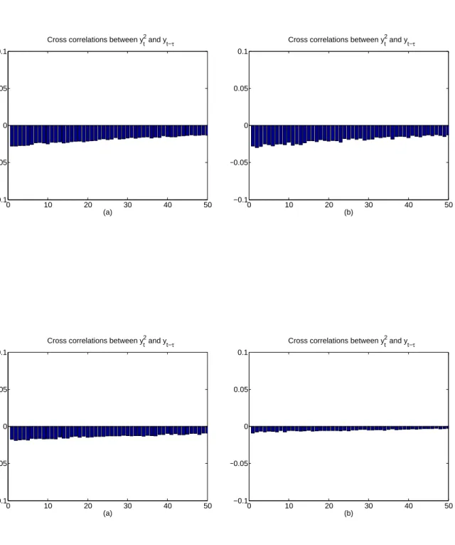
Finally, A-ARSV does systematically better than LL1VF, although the differences in MSE and MAE in Table 8 are rather small. To analyze their relative performance, we focus on the two features of the LL1VF model that differ the most from the A-ARSV model: the leverage specification and the volatility feedback. Regarding leverage, while LL1VF considers instantaneous correlations, A-ARSV models correlation between lagged returns and volatility directly. To asses wether leverage could play a role in explaining the difference in performance for the Microsoft series, we have simulated data taking the parameter estimates to be the data generating process for both models. Figure 3 shows the numerical approximation to the lagged correlations based on these simulations. It turns out that the estimated LL1VF model generates substantially less leverage than the estimated A-ARSV. In light of this result, a third conclusion is that alternative mechanisms to incorporate leverage in the LL1VF model might improve the forecast performance. In this direction, there is evidence of the good performance of the A-ARSV leverage specification. Yu (2005) compares it to an alternative specification in the context of discrete-time stochastic volatility models and concludes that the alternative is inferior from both a theoretical and empirical point of view.

On the other hand, the volatility feedback is estimated to be very small in the case of Microsoft and we argue below that it can only play, if any, a small role. As noted in Section 2, volatility feedbacks introduce a lower bound for the volatility in the LL1VF model. The Microsoft instantaneous standard deviation has a lower bound implied by the in-sample parameter estimates of 5.093×10−7, extremely close to its natural lower bound of zero. However, a non-zero lower bound can be critical for out-of-sample performance if there is a large enough drop in volatility.

Note that the out-of-sample volatility pattern differs from that of the in-sample period (see Figure 1). Shortly before the out-of-sample period begins, there seems to be a drop in volatility that persists over the whole out-of-sample period. A closer look at Figure 2 would suggest that this drop is more severe for Coca-Cola and Disney, for which there seems to be a small but constant decline in the volatility throughout the out-of-sample period.

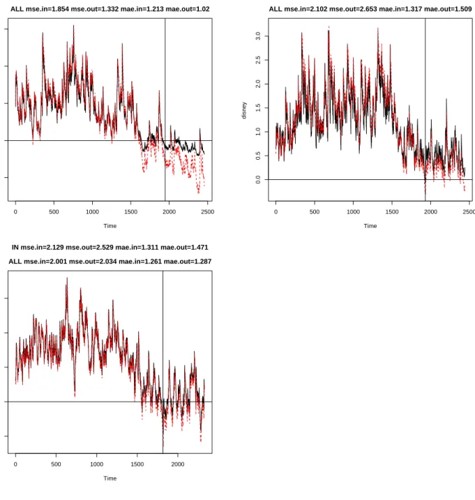
For Coca-Cola, the LL1VF forecasting accuracy is substantially worse than that of other time models, including the A-ARSV (see Tables 6 and 10). In particular, all discrete-time models systematically outperform the LL1VF. As for Microsoft, we look into the factors that might explain this worse performance of LL1VF. The LL1VF seems to produce, based on in-sample estimates, similar cross-correlations between squared observations and past returns to those generated by the A-ARSV (see Figure 3). This suggests checking whether, unlike for Microsoft, the volatility feedback causes an undesired volatility lower bound that prevents the forecasts from following the out-of-sample drop in volatility. Indeed, the lower bound on the instantaneous standard deviation implied by the in-sample point estimates is 5.938. The sharp effect of such lower bound can be appreciated in Figure 4. The one-step ahead forecasts based on the in-sample parameter estimates are higher than those based on estimates using all the available data, the latter being able to track the out-of-sample drop in volatility. The instantaneous standard deviation lower bound obtained with parameter estimates based on

all the data (in-sample and out-of-sample) is 1.346, much lower than the bound implied by the in-sample point estimates.

For Disney, LL1VF does not seem to be able to reproduce the amount of leverage of A-ARSV (as it happens for Microsoft), and the in-sample lower bound of 1.947 seems to be more of a problem than that of Microsoft but less than that of Coca-Cola. We should not be surprised that the LL1VF is outperformed by the A-ARSV and that its relative performance to other discrete-time models is slightly better than the one for Coca-cola but not as good as the one for Microsoft.

Another remark based on the Disney and, mostly, on the Coca-Cola series is that mecha-nisms alternative to volatility feedbacks may substantially improve the forecast performance of continuous-time models. Investigating such alternative mechanisms falls outside the scope of this paper, where we focus on the forecast ability comparison. However, there is good evidence supporting volatility feedbacks, including the fits reported in Chernov et al. (2003) or in Durham (2007), besides our own Coca-Cola and Disney fits. Hence, mechanisms of a similar nature but that avoid imposing volatility lower bounds seem to be a promising target. Finally, a result consistent across all our investigations is that A-ARSV outperforms

LL1VF systematically. To better understand the comparison between these two models,

we evaluate them in terms of in-sample volatility filtering. Table 9 presents these results. A-ARSV seems to do better than LL1VF for the three stocks but the differences are substan-tially smaller than those in out-of-sample forecasting for Coca-Cola and for Disney. A more careful analysis based on approximate standard errors shows that this difference can hardly be taken to be statistically significant. This leads us to conclude that the in-sample filtering accuracies of both models are similar. This is in agreement with our previous interpretation that the volatility lower bound implied by in-sample parameter estimates, in combination with an out-of-sample volatility drop, could be determining the worse forecast performance of LL1VF for Coca-cola and Disney.

6

Conclusion

In this paper we have compared the forecast performance of continuous and discrete-time volatility models using predictive ability tests for three well-known international stocks con-sidering three performance measures. We have considered more than ten GARCH-type models with errors following either a normal, Student-t or skew-t distribution and an asymmetric au-toregressive stochastic volatility model with errors following a normal distribution. We have compared these models to a continuous-time stochastic volatility model with mean reversion, volatility feedback and leverage.

We have estimated each model by maximum likelihood using, for the two stochastic volatil-ity models, the iterated filtering algorithm implemented using particle filters. As a proxy of the ex-post volatility, we have chosen the two scales realized volatility by Zhang et al. (2005), which is calculated on intra-day 10-minutes returns and minimizes the biases caused by market microstructure noise.

volatil-ity forecasts than simpler discrete-time models, like GARCH; (ii) for more sophisticated discrete-time alternatives, including long memory or leverage, continuous-time models may also do better; but (iii) within the stochastic volatility family, there is no evidence that a continuous-time model can outperform a discrete-time model. Due to the computational bur-den, the comparison has been unequal, giving much more weight to GARCH-type models than to stochastic volatility models. More work focusing on the latter would complement our investigations.

This work should be considered a first attempt in the literature to evaluate the volatility forecast performance of continuous-time compared to discrete-time. Nevertheless, we interpret (i) and (ii) as evidence that, besides other merits of continuous-time models, they may be used as a tool for generating reasonable volatility forecasts.

Also, the discrete-time models that have performed better in the empirical forecast com-parison indicate directions in which it seems advisable to extend the continuous-time specifi-cation. In particular, the volatility feedback may have serious drawbacks if there is a drop in volatility that fall below the volatility lower bound implied by the model. Another direction that could provide a substantial improvement in forecast accuracy is including an asymmetric, possibly with heavy tails, distribution for the noises. Finally, modifying the way the lever-age is modeled could also improve the performance of continuous-time models. Investigating extensions along these lines falls outside the scope of this paper.

References

A¨ıt-Sahalia, Y. and R. Kimmel (2007). Maximum likelihood estimation of stochastic volatility models. Journal of Financial Economics 134, 507–551.

A¨ıt-Sahalia, Y. and L. Mancini (2008). Out of sample forecasts of quadratic variation.Journal of Econometrics 147, 17–33.

Amin, K. and V. Ng (1997). Inferring future volatility from the information in implied volatility in eurodollar options: A new approach. Review of Financial Studies 10, 333–367.

Andersen, T. and T. Bollerslev (1998). Answering the skeptics: Yes, standard volatility models do provide accurate forecasts. International Economic Review 39, 885–905.

Andersen, T., T. Bollerslev, P. Christoffersen, and F. Diebold (2005). Volatility forecasting.

CFS Working Paper.

Andersen, T., T. Bollerslev, F. Diebold, and P. Labys (2003). Modelling and forecasting realized volatility. Econometrica 71, 579–625.

Andreou, E. and E. Ghysels (2002). Rolling-sample volatility estimators: Some new theo-retical, simulation, and empirical results. Journal of Business and Economic Statistics 20, 363–376.

Bai, C., J. Russel, and G. Tiao (2004). Effects of non-normality and dependence on the preci-sion of variance estimates using high-frequency financial data. Working Paper, University of Chicago.

Barndorff-Nielsen, O. and N. Shephard (2004). Econometric analysis of realized covaria-tion: High frequency based covariance, regression, and correlation in financial economics.

Econometrica 72, 885–925.

Bluhm, H. and J. Yu (2002). Forecasting volatility: Evidence from the german stock market.

Research Collection School of Economics, P 1113.

Bret´o, C., D. He, E. Ionides, and A. King (2009). Time series analysis via mechanistic models.

Annals of Applied Statistics 3, 319–348.

Brockwell, P., E. Chadraa, and A. Lindner (2006). Continuous-time GARCH processes. The Annals of Applied Probability 16, 790–826.

Broto, C. and E. Ruiz (2004). Estimation methods for stochastic volatility models: A survey.

Journal of Economic Surveys 18, 613–649.

Carnero, M., D. Pe˜na, and E. Ruiz (2007). Effects of outliers on the identification and estimation of GARCH models. Journal of Time Series Analysis 28, 471–497.

Chernov, M., A. R. Gallant, E. Ghysels, and G. Tauchen (2003). Alternative models for stock price dynamics. Journal of Econometrics 116, 225–257.

Davidson, J. (2004). Moment and memory properties of linear conditional heteroscedasticity models, and a new model. Journal of Business and Economic Statistics 22, 16–29.

Doucet, A., N. de Freitas, and N. J. Gordon (Eds.) (2001). Sequential Monte Carlo Methods in Practice. New York: Springer.

Durham, G. (2007). SV mixture models with application to S&P 500 index returns. Journal of Financial Economics 85, 822–856.

Ederington, L. and W. Guan (2005). Forecasting volatility. Journal of Futures Markets 25, 465–490.

Gallant, A. R. and G. Tauchen (1996). Which moments to match? Econometric Theory 12, 657–681.

Giacomini, R. and H. White (2006). Tests of conditional predictive ability. Econometrica 74, 1545–1578.

Gouri´eroux, C. and A. Monfort (1996). Simulation-based econometric methods. Oxford Uni-versity Press.

Gran´e, A. and H. Veiga (2008). Accurate minimum capital risk requirements: a comparison of several approaches. Journal of Banking and Finance 32, 2482–2492.

Granger, C. and R. Joyeux (1980). An introduction to long memory time series models and fractional differencing. Journal of Time Series Analysis 1, 15–29.

Hansen, P. and A. Lunde (2005). A forecast comparison of volatility models: Does anything beat a garch(1,1)? Journal of Applied Econometrics 20, 873–889.

Hansen, P. and A. Lunde (2006). Realized variance and market microstructure noise. Journal of Business and Economic Statistics 24, 127–161.

Harvey, A. and N. Shephard (1996). Estimation of an asymmetric stochastic volatility model for asset returns. Journal of Business and Economic Statistics 4, 429–434.

He, D., E. Ionides, and A. King (2010). Plug-and-play inference for disease dynamics: Measles in large and small populations as a case study. Journal of the Royal Society Interface 7, 271–283.

Ionides, E., C. Bret´o, and A. King (2006). Inference for nonlinear dynamical systems. Pro-ceedings of the National Academy of Science 49, 18438–18443.

Ionides, E. L., A. Bhadra, Y. Atchad´e, and A. A. King (2011). Iterated filtering. Annals of Statistics Pre-published online.

Johannes, M., N. Polson, and J. Stroud (2009). Optimal filtering of jump diffusions: Extract-ing latent states from asset prices. Review of Financial studies 22, 2759–2799.

Jones, C. (2003). The dynamics of stochastic volatility.Journal of Econometrics 116, 181–224.

King, A., E. Ionides, M. Pacual, and M. Bouna (2008). Inapparent infections and cholera dynamics. Nature 454, 877–880.

King, A. A., E. L. Ionides, C. Bret´o, S. Ellner, B. Kendall, H. Wearing, M. J. Ferrari, M. Lavine, and D. C. Reuman (2010). pomp: Statistical inference for partially observed Markov processes (R package).

Koopman, S., B. Jungbacker, and E. Hol (2005). Forecasting daily variability of the s&p 100 stock index using historical, realised and implied volatility measurements. Journal of Empirical Finance 12, 445–475.

Laurent, S. and J. Peters (2006). G@RCH 4.2, Estimating and Forecasting ARCH Models. Timberlake Consultants.

Merton, R. (1969). Lifetime portfolio selection under uncertainty: The continuous time case.

Review of Economics and Statistics 51, 247257.

Merton, R. (1971). Optimum consumption and portfolio rules in a continuous time model.

Journal of Economic Theory 3, 373413.

Merton, R. (1980). On estimating the expected return on the market: An exploratory inves-tigation. Journal of Financial Economics 8, 323–361.

Nelson, D. B. (1991). Conditional heteroskedasticity in asset returns: A new approach.

Econometrica 59, 347–370.

Oomen, R. (2002). Modelling realized variance when returns are serially correlated. Working Paper,Warwick Business School.

Pagan, A. and W. Schwert (1990). Alternative models for conditional stock volatility. Journal of Econometrics 45, 267–290.

Parzen, E. (1981). Time Series Model Identification and Prediction Variance Horizon. in Applied Time Series Analysis II, ed. Findley, Academic Press, New York.

R Development Core Team (2010). R: A Language and Environment for Statistical Comput-ing. Vienna, Austria: R Foundation for Statistical Computing. ISBN 3-900051-07-0.

Ruiz, E. and H. Veiga (2008). Modelos de volatilidad estoc´astica: una alternativa atractiva y factible para modelizar la evoluci´on de la volatilidad. Anales de Estudios Econ´omicos y Empresariales XVIII, 1–59.

Stinchcombe, M. and H. White (1998). Consistent speci.cation testing with nuisance param-eters present only under the alternative. Econometric Theory 14, 295–324.

Sundaresan, S. (2000). Continuous-time methods in finance: A review and an assessment.

The Journal of Finance LV, 1569–1622.

Taylor, S. (1994). Modelling stochastic volatility: A review and comparative study. Mathe-matical Finance 4, 183–204.

West, K. and D. Cho (1995). The predictive ability of several models of exchange rate volatility. Journal of Econometrics 69, 367–391.

Yang, M. (2011). Volatility feedback and risk premium in GARCH models with generalized hyperbolic distributions. Studies in Nonlinear Dynamics & Econometrics 15, article 6, 1–19.

Yu, J. (2005). On leverage in a stochastic volatility model. Journal of Econometrics 127, 165–178.

Zhang, L., P. Mykland, and Y. A¨ıt-Sahalia (2005). A tale of two time scales: Determining integrated volatility with noisy high frequency data. Journal of the American Statistical Association 100, 1394–1411.

Zhou, B. (1996). High-frequency data and volatility in foreign-exchange rates. Journal of Business and Economic Statistics 14, 45–52.

Appendix: Forecasting volatility with the GARCH-type models

Unlike for the A-ARSV and LL1VF models, the one-step ahead prediction and filter means coincide for the GARCH-type models, since for these models volatility is assumed to be ob-served one-step ahead, i.e. E

h σ_t2 U1,1:t i = E h σ_t2 U1,1:t−1 i

. This assumption also implies that either the prediction or filtering mean of any transformation of the volatility is sim-ply the transformation of the mean of the volatility, i.e. for example Ehln (σ_t2)

U1,1:t−1 i = lnEhσ_t2 U1,1:t−1 i

. Therefore, in the remainder of this section we only describe how the volatility forecasts were obtained.

GARCH(1,1): Using recursive substitutions, the GARCH(1,1) model can be written as an ARCH(∞); that is,

σ_t2 =ω(1−β)−1+α

+∞

X

i=1

βi−1ε2_t−i. (I) The one-step ahead forecast of the conditional variance based upon the available informa-tion is given by σ2_t+1|GARCH =ω(1−β)−1+α +∞ X i=1 βi−1ε2_t−i. (II)

EGARCH(1,1): The EGARCH model parameterizes the conditional variance in terms of logarithms, that is

ln(σ2)t+1|EGARCH =ω+γ1(|t| −E(|t|)) +γt+γ2ln(σ2)t|EGARCH, (III)

where t = εtσ_t−_|EGARCH1 . As pointed out by Andersen et al. (2005), the EGARCH delivers

the smallest mean square error forecasts for the future logarithmic conditional variances.

FIGARCH(1, d,1): If we consider a FIGARCH(1, d,1), then the one-step ahead condi-tional variance forecast is given by

σ_t2_{+1|F IGARCH} =ω(1−β)−1+λ(L)σ_t2_{|F IGARCH}, (IV) where the coefficients of λ(L) = 1−(1−βL)−1(1−αL−βL)(1−L)d are computed from expressionsλ1 =α+dand

λj =βλj−1+ [(j−1−d)j−1−(α+β)]δj−1, with δj ≡δj−1(j−1−d)j−1. (V)

forj >1. Note that theδj’s are the coefficients in the Maclaurin series expansion of (1−L)d

Tables and Figures

Coca−cola Time 0 100 200 300 400 500 0.02 0.05 0.20 0.50 2.00 5.00 20.00 Disney Time 0 100 200 300 400 500 0.02 0.05 0.20 0.50 2.00 5.00 20.00 Microsoft Time 0 100 200 300 400 500 0.02 0.05 0.20 0.50 2.00 5.00 20.00

0 10 20 30 40 50 −0.1 −0.05 0 0.05 0.1

Cross correlations between y2_t and y_t−τ

(a) 0 10 20 30 40 50 −0.1 −0.05 0 0.05 0.1 (b)

Cross correlations between y2_t and y_t−τ

0 10 20 30 40 50 −0.1 −0.05 0 0.05 0.1

Cross correlations between y2 t and yt−τ (a) 0 10 20 30 40 50 −0.1 −0.05 0 0.05 0.1

Cross correlations between y2 t and yt−τ

(b)

Figure 3: Cross correlations between simulated squared returns and past simulated returns for the Coca-cola (first row) and Disney (second row) fits. (a) A-ARSV and (b) LL1VF.

Time cola 0 500 1000 1500 2000 2500 −1 0 1 2 3

IN mse.in=1.743 mse.out=2.521 mae.in=1.178 mae.out=1.488 ALL mse.in=1.854 mse.out=1.332 mae.in=1.213 mae.out=1.02

Time disne y 0 500 1000 1500 2000 2500 0.0 0.5 1.0 1.5 2.0 2.5 3.0

IN mse.in=1.836 mse.out=3.219 mae.in=1.212 mae.out=1.692 ALL mse.in=2.102 mse.out=2.653 mae.in=1.317 mae.out=1.509

Time micro 0 500 1000 1500 2000 −1 0 1 2 3

IN mse.in=2.129 mse.out=2.529 mae.in=1.311 mae.out=1.471 ALL mse.in=2.001 mse.out=2.034 mae.in=1.261 mae.out=1.287

Figure 4: Forecast performance of the LL1VF model. The figures show the in-sample and the out-of-sample (separated by the vertical line) one-step ahead inferred volatilities by the LL1VF model. We only show the in-sample volatilities for which we had TSRV data. The title of the plot shows the MSE and MAE in the out-of-sample period and in the in-sample period for which TSRV data was available. The solid line uses point estimates obtained with the in-sample data (3534 observations). The dashed line uses point estimates obtained using all the available data (4046 observations).

T able 1: Co ca-Cola GAR CH-t yp e mo dels’ estimation results Final GAR CH-t yp e mo dels’estimates and standard deviations for Co ca-Cola data co v ering the p erio d Jan uary 2, 1991 till Jan uary 22, 2007. Mo dels cst (mean) cst (v ar) α β DF Asym T ail d γ1 γ2 loglik GAR CH -7017.331 Estimates 0.059 0.004 0.036 0.963 Std. Dev. (0.019 ) (0.004) (0.014) (0.014) GAR CH-T -6910.649 Estimates 0.038 0.002 0.028 0.971 6.890 Std. Dev. (0.018 ) (0.002) (0.006) (0.007) (0.689) GAR CH-SK -6904.727 Estimates 0.055 0.002 0.028 0.971 0 .080 6.771 Std. Dev. (0.018 ) (0.002) (0.006) (0.007) (0.025) (0.670) EGAR CH -6999.244 Estimates 0.041 1.426 -0.556 0.9 96 -0.0 61 0.203 Std. Dev. (0.016 ) (0.585) (0.130) (0.002) (0.019) (0.051) EGAR CH-SK -6888.641 Estimates 0.038 4.046 -0.541 0.9 97 0.078 7.12 9 -0.066 0.205 Std. Dev. (0.018 ) (2.150) (0.107) (0.002) (0.025) (0.743) (0.017) (0.039) FIGAR CH -7005.198 Estimates 0.060 0.023 0.527 0.781 0.408 Std. Dev. (0.019 ) (0.012) (0.072) (0.055) (0.043) FIGAR CH-T -6905.454 Estimates 0.04 0.015 0.501 0.793 7.507 0.431 Std. Dev. (0.018 ) (0.009) (0.048) (0.038) (0.758) (0.041) FIGAR CH-SK -6898.903 Estimates 0.056 0.015 0.500 0.794 0 .083 7.389 0.433 Std. Dev. (0.018 ) (0.009) (0.047) (0.037) (0.024) (0.736) (0.040)

T able 2: Disney GAR CH-t yp e mo dels’ estimation results Final GAR CH-t yp e mo dels’estimates and standard deviations for Disney data co v ering the p erio d Jan uary 2, 1991 till Jan uary 22, 2007. Mo d els cst (m ean) cst (v ar) α β DF Asym T ail d γ1 γ2 loglik GAR CH -7994.621 Estimates 0.062 0.010 0.0 29 0.968 Std. Dev. (0.025) (0.007) (0.008) (0.010) GAR CH-T -7908.466 Estimates 0.039 0.008 0.0 24 0.973 7.151 Std. Dev. (0.024) (0.005) (0.006) (0.007) (0.752) GAR CH-SK -7904.313 Estimates 0.060 0.007 0.0 24 0.974 0.06 6 7.144 Std. Dev. (0.025) (0.005) (0.006) (0.007) (0.024) (0.746) EGAR CH -7973.021 Estimates 0.038 1.656 -0.664 0.996 -0.059 0.215 Std. Dev. (0.025) (0.335) (0.091) (0.002) (0.019) (0.042) EGAR CH-T -7886.937 Estimates 0.019 1.076 -0.718 0.997 7.534 -0.075 0.241 Std. Dev. (0.024) (0.344) (0.069) (0.001) (0.842) (0.018) (0.041) EGAR CH-SK -7883.813 Estimates 0.035 2.908 -0.718 0.997 0.057 7.573 -0.072 0.237 Std. Dev. (0.025) (1.174) (0.069) (0.002) (0.024) (0.837) (0.018) (0.040) FIGAR CH -7991.427 Estimates 0.058 0.352 0.4 68 0.696 0.352 Std. Dev. (0.025) (0.052) (0.116) (0.117) (0.052) FIGAR CH-T -7902.747 Estimates 0.037 0.087 0.5 21 0.726 7.379 0.346 Std. Dev. (0.024) (0.044) (0.100) (0.096) (0.776) (0.046) FIGAR CH-SK -7898.855 Estimates 0.056 0.091 0.5 14 0.718 0.06 3 7.398 0.342 Std. Dev. (0.025) (0.047) (0.105) (0.102) (0.024) (0.769) (0.045)

T able 3: Microsoft GAR CH-t yp e mo dels’ estimation results Final GAR CH-t yp e mo dels’estimates and standard deviations for Disney data co v ering the p erio d Jan uary 2, 1991 till Jan uary 22, 2007. Mo dels cst (mean) cst (v ar) α β DF Asym T ail d γ1 γ2 loglik GAR CH -8401.584 Estimates 0.092 0.015 0.055 0 .943 Std. Dev. (0.027) (0.009) (0.014) (0.014) GAR CH-T -8310.888 Estimates 0.056 0.009 0.058 0 .943 6.779 Std. Dev. (0.025) (0.007) (0.017) (0.016) (0.67 0) GAR CH-SK -8305.101 Estimates 0.081 0.010 0.060 0 .941 0.075 6.7 40 Std. Dev. (0.026) (0.008) (0.018) (0.017) (0.023) (0.6 60) EGAR CH-SK -8292.674 Estimates 0.070 3.515 0.992 0.075 6.897 -0.024 0.154 Std. Dev. (0.027) (0.988) (0.003) (0.023) (0.681) (0.010) (0.026) FIGAR CH -8395.001 Estimates 0.097 0.067 0.295 0 .643 0.439 Std. Dev. (0.027) (0.038) (0.075) (0.085) (0.055) FIGAR CH-T -8304.808 Estimates 0.060 0.039 0.275 0 .658 7.393 0.471 Std. Dev. (0.025) (0.026) (0.051) (0.055) (0.69 6) (0.044) FIGAR CH-SK -8297.854 Estimates 0.084 0.041 0.263 0 .646 0.081 7.3 65 0.468 Std. Dev. (0.026) (0.026) (0.051) (0.055) (0.022) (0.6 89) (0.043) FIEGAR CH-SK -8277.135 Estimates 0.059 2.630 0.613 0.046 7.235 0.569 -0.028 0.152 Std. Dev. (0.025) (0.356) (0.134) (0.014) (0.750) (0.051) (0 .012) (0.032)

Table 4: LL1VF models’ estimation results

Final LL1VF parameter estimates along with standard errors. The data covers the period January 2, 1991 till January 22, 2007.

Model/Series α10 β10 β12 α22 β22 ψ12 loglik COCA-COLA -6938.765 Estimates 15.125 3.346 1.061 -0.893 0.348 -0.301 Std. Errors (5.434) (0.115) (0.088) (0.379) (0.047) (0.077) DISNEY -7937.604 Estimates 13.838 3.467 0.981 -1.365 0.493 -0.096 Std. Errors (6.253) (0.135) (0.186) (0.508) (0.055) (0.070) MICROSOFT -8319.219 Estimates 22.765 3.245 1.365 -4.511 0.037 -0.084 Std. Errors (7.600) (0.062) (0.105) (1.011) (0.118) (0.062)

Table 5: A-ARSV models’ estimation results

Final A-ARSV parameter estimates along with standard errors. The data covers the period January 2, 1991 till January 22, 2007.

Model/Series µ σ∗ φ1 rh δ loglik COCA-COLA -6930.252 Estimates 0.048 1.490 0.990 0.130 -0.394 Std. Errors (0.017) (0.062) (0.004) (0.009) (0.022) DISNEY -7931.720 Estimates 0.061 1.532 0.990 0.116 -0.290 Std. Errors (0.022) (0.070) (0.004) (0.009) (0.022) MICROSOFT -8312.881 Estimates 0.047 1.711 0.983 0.157 -0.203 Std. Errors (0.024) (0.073) (0.005) (0.011) (0.036)

T able 6: Co ca-Cola out-of-sample mo del’s forecast p erformance One-step-ahead v olatilit y forecas ts. P anel A sho ws the forecasting results without re-estimating the mo dels and panel B sho ws the forecasting results re-estimating the mo dels. Mo del’s forecasts are ev aluated against TSR V. The ev aluation p erio d is Jan uary 7, 2005 till Jan uary 22, 2007. ( ∗ ) refers to results of the second loss function. Mo dels F orecast Loss F unctions F orecast Loss F unctions P anel A P anel B MSE MSE ( ∗ ) MAE MAE ( ∗ ) R 2 R 2( ∗ ) MSE MSE ( ∗ ) MAE MAE ( ∗ ) R 2 R 2( ∗ ) GAR CH 0.202 2.273 0.430 1.404 0.103 0.105 0.148 1.795 0.359 1.224 0.122 0.125 GAR CH-T 0.188 2.168 0.414 1.366 0.102 0.103 0.139 1.727 0.348 1.199 0.131 0.134 GAR CH-SK 0.188 2.166 0.414 1.366 0.105 0.106 0.140 1.734 0.349 1.202 0.134 0.136 EGAR CH 0.162 1.923 0.385 1.292 0.236 0.251 0.132 1.636 0.341 1.177 0.229 0.243 EGAR CH-SK 0.156 1.859 0.376 1. 268 0.237 0.250 0.130 1.606 0.337 1.170 0.235 0.249 FIGAR CH 0.171 1.991 0.394 1.312 0.196 0.196 0.158 1.851 0.375 1.260 0.214 0.214 FIGAR CH-T 0.171 1.991 0.394 1.312 0.196 0.196 0.143 1.730 0.355 1.210 0.206 0.206 FIGAR CH-SK 0.173 2.008 0.397 1.319 0.198 0.199 0.145 1.746 0.358 1.217 0.209 0.209 A-ARSV 0.185 1.942 0.405 1.284 0.127 0.143 0.151 1.634 0.354 1.152 0.135 0.151 LL1VF 0.245 2.521 0.477 1.488 0.093 0.103 0.183 1.993 0.401 1.301 0.114 0.124

T able 7: Disney out-of-sample mo del’ s forecast p erformance One-step-ahead v olatilit y forecas ts. P anel A sho ws the forecasting results without re-estimating the mo dels and panel B sho ws the forecasting results re-estimating the mo dels. Mo del’s forecasts are ev aluated against TSR V. The ev aluation p erio d is Jan uary 7, 2005 till Jan uary 22, 2007. ( ∗ ) refers to results of the second loss function. Mo dels F orecas t Loss F unctions F orecast Loss F unctions P anel A P anel B MSE MSE ( ∗ ) MAE MAE ( ∗ ) R 2 R 2( ∗ ) MSE MSE ( ∗ ) MAE MAE ( ∗ ) R 2 R 2( ∗ ) GAR CH 0.519 3.093 0.694 1.657 0.030 0.029 0.502 3.028 0.682 1.638 0.030 0.030 GAR CH-T 0.515 3.084 0.692 1.654 0.026 0.025 0.499 3.023 0.680 1.636 0.030 0.029 GAR CH-SK 0.514 3.082 0.692 1.654 0.027 0.026 0.498 3.021 0.680 1.636 0.031 0.030 EGAR CH 0.453 2.797 0.649 1.580 0.143 0.146 0.447 2.776 0.645 1.573 0.143 0.146 EGAR CH-T 0.434 2.711 0.634 1.553 0.147 0.151 0.432 2.707 0.633 1.552 0.148 0.152 EGAR CH-SK 0.432 2.704 0.632 1.551 0.147 0.151 0.431 2.701 0.632 1.550 0.148 0.152 FIGAR CH 0.593 3.317 0.747 1.734 0.100 0.117 0.562 3.200 0.725 1.699 0.097 0.112 FIGAR CH-T 0.577 3.253 0.735 1.714 0.105 0.121 0.551 3.153 0.717 1.686 0.104 0.119 FIGAR CH-SK 0.581 3.267 0.738 1.720 0.106 0.123 0.554 3.165 0.719 1.690 0.105 0.121 A-ARSV 0.582 2.980 0.723 1.617 0.045 0.055 0.543 2.916 0.700 1.598 0.045 0.049 LL1VF 0.620 3.219 0.754 1.692 0.029 0.036 0.568 6.520 0.724 2.482 0.026 0.028

T able 8: Microsoft out-of-sample mo del’s forecast p erformance One-step-ahead v olatilit y forecas ts. P anel A sho ws the forecasting results without re-estimating the mo dels and panel B sho ws the forecasting results re-estimating the mo dels. Mo del’s forecasts are ev aluated against TSR V. The ev aluation p erio d is Jan uary 7, 2005 till Jan uary 22, 2007. ( ∗ ) refers to results of the second loss function. Mo dels F orecast Loss F unctions F orecast Loss F unctions P anel A P anel B MSE MSE ( ∗ ) MAE MAE ( ∗ ) R 2 R 2( ∗ ) MSE MSE ( ∗ ) MAE MAE ( ∗ ) R 2 R 2( ∗ ) GAR CH 0.475 3.051 0.658 1.647 0.133 0.147 0.357 2.478 0.556 1.457 0.118 0.134 GAR CH-T 0.408 2.720 0.601 1.543 0.130 0.143 0.331 2.323 0.528 1.400 0.117 0.133 GAR CH-SK 0.415 2.756 0.607 1.553 0.134 0.149 0.338 2.358 0.535 1.414 0.122 0.138 EGAR CH-SK 0.424 2.734 0.612 1.553 0.189 0.199 0.350 2.378 0.546 1.429 0.171 0.181 FIGAR CH 0.424 2. 833 0.621 1.585 0.158 0.181 0.343 2.423 0.548 1.448 0.149 0.170 FIGAR CH-T 0.378 2.592 0.579 1.507 0.159 0.181 0.312 2.237 0.515 1.381 0.148 0.170 FIGAR CH-SK 0.381 2.609 0.583 1.512 0.159 0.182 0.315 2.254 0.519 1.387 0.148 0.170 FIEGAR CH-SK 0.262 2.038 0.477 1.316 0.191 0.203 0.250 1.965 0.464 1.287 0.184 0.198 A-ARSV 0.419 2.460 0.596 1.449 0.147 0.160 0.368 2.257 0.552 1.374 0.135 0.144 LL1VF 0.435 2.529 0.607 1.471 0.1346 0.151 0.397 2.372 0.575 1.413 0.125 0.138

T able 9: In-sample filtering mo del p erformance P anel A sho ws the v alues of the filtering loss functions ev aluated in-sample. P anel B sho ws the standard errors corresp onding to the MSE and MAE sample statistics. Losses are ev aluated against TSR V. The ev aluation p erio d is sligh tly differen t for eac h series (due differen t a v ailable data) and go es from around Jan u ary of 1997 to Jan uary of 2005, i.e., appro ximately 2000 daily observ ations for eac h series. ( ∗ ) refers to results of the second loss fu nction. Mo dels Loss F unctions Standard Errors P anel A P anel B MSE MSE ( ∗ ) MAE MAE ( ∗ ) R 2 R 2( ∗ ) MSE MSE ( ∗ ) MAE MAE ( ∗ ) R 2 R 2( ∗ ) Co ca-Cola A-ARSV 0.604 1.608 0.688 1.133 0.42 0.468 0.014 0.034 0.008 0.013 NA NA LL1VF 0.717 1.715 0.734 1.174 0.406 0.459 0.021 0.035 0.01 0.013 NA NA Disney A-ARSV 1.029 1.737 0.908 1.184 0.37 0.458 0.024 0.036 0.01 0.013 NA NA LL1VF 1.115 1.811 0.937 1.21 0.351 0.44 0.029 0.037 0.011 0.013 NA NA Microsof A-ARSV 1.404 2.073 1.04 1.298 0.405 0.508 0.041 0.042 0.013 0.015 NA NA LL1VF 1.449 2.108 1.056 1.309 0.395 0.501 0.042 0.043 0.014 0.015 NA NA