Solving the integrated airline recovery problem using
column-and-row generation
Stephen J Maher
School of Mathematics and Statistics, University of New South Wales, Sydney NSW 2052, Australia.
Abstract
Airline recovery presents very large and difficult problems requiring high quality solutions within very short time limits. To improve computational performance, various solution approaches have been employed, including decomposition methods and approximation techniques. There has been increasing interest in the development of efficient and accurate solution techniques to solve an inte-grated airline recovery problem. In this paper, an inteinte-grated airline recovery problem is developed, integrating the schedule, crew and aircraft recovery stages, and is solved using column-and-row generation. A general framework for column-and-row generation is presented as an extension of cur-rent generic methods. This extension considers multiple secondary variables and linking constraints and is proposed as an alternative solution approach to Benders’ decomposition. The application of column-and-row generation to the integrated recovery problem demonstrates the improvement in the solution runtimes and quality compared to a standard column generation approach. Column-and-row generation improves solution runtimes by reducing the problem size and thereby achieving faster execution of each LP solve. As a result of this evaluation, a number of general enhancement techniques are identified to further reduce the runtimes of column-and-row generation. This paper also details the integration of the row generation procedure with branch-and-price, which is used to identify integral optimal solutions.
Key words: airline recovery, column generation, row generation
1
Introduction
Disruptions are very common in the airline industry, greatly impacting the realised operational perfor-mance. To mitigate the effect of these disruptions, intervention by the airline is necessary to maintain the many operational requirements of aircraft and crew. Consequently, any disruption results in a sig-nificant increase to an airlines operational costs related to additional crew overtime and increased fuel usage. Due to the significant associated costs, the use of efficient and accurate recovery processes is of great importance to the airline industry.
1 INTRODUCTION 2
The airline recovery problem, similar to the planning problem, is a very large and complex problem commonly broken into a number of smaller, more tractable sequential stages. These stages are broadly categorised as schedule, aircraft, crew and passenger recovery, also defining clear boundaries for research in this area. The complete recovery process is a sequential problem, where each stage is solved to optimality and fixed for use in subsequent stages. Analogous to the planning problem, this typically results in suboptimal, or even infeasible, solutions due to little interaction between the stages. The integration of two or more stages in the planning problem has been demonstrated to provide higher quality solutions [15, 25, 29], as such there is a similar expectation for airline recovery. The focus of this paper is an integrated airline recovery problem, integrating the schedule, aircraft and crew recovery.
A critical constraint on the airline recovery problem is the allowable time limit to find an optimal solution. Generally the solution to the airline recovery problem is required within minutes of a disruptive event, prompting the development of many solution approaches to achieve this. The proposed solution approaches to achieve improved runtime performance varies between each of the recovery stages. The integration of multiple recovery stages presents very difficult and complex problems, which are commonly solved with the use of decomposition techniques. Unfortunately, the decomposition techniques employed, such as Benders’ decomposition, do not provide a guarantee of integral optimality. A contribution of this paper is the development of a column-and-row generation framework as an exact solution approach to solve the integrated airline recovery problem.
1.1
Airline recovery literature
The most common method employed to improve the runtimes of the aircraft recovery problem is through the network design. There are three classes of network design that have been employed, the time-line, time-band and connection networks. The time-line network is a very popular approach used for the aircraft recovery problems, with Jarrah et al. [20] presenting an early example using this network description. The work of [20] is extended by Cao and Kanafani [12, 13], integrating the two models developed by [20] and implementing additional recovery policies. The use of the time-line network is developed further by Yan and Yang [40], presenting a unique design that concisely describes the effect of airline disruptions on the planned schedule. The time-band network is presented by Arg¨uello [6] to approximate the flight network by aggregating activities at airports into discrete time bands. Therefore, the number of nodes used to define the recovery network is reduced. This network description has been demonstrated by Bardet al.[8] and Eggenberg et al.[16] to improve the solution runtimes of the aircraft recovery problem. Finally, Rosenbergeret al.[31] present an aircraft recovery problem using the classical connection network, which provides a concise description of the recovery flight schedule. Given the potential size of this problem, the authors employ a heuristic to select a minimal number of aircraft to include in the model for possible rerouting.
1 INTRODUCTION 3
operational cost of an airline. Similar to the aircraft recovery problem, a number of unique approaches have been proposed to improve solution runtimes. These approaches involve reducing the problem size by selecting only a subset of crew and flights, fixing the flight schedule by using the solution to the aircraft recovery problem (part of the sequential recovery process), or implementing only a selection of recovery policies.
Solving the crew recovery problem with a fixed flight schedule is first presented by Wei et al. [39], attempting to repair any pairings affected by a schedule disruption. Fast solution runtimes are achieved with the use of a branch-and-bound heuristic designed with consideration to the actions of an AOCC. Another approach using a fixed flight schedule is the crew rescheduling problem proposed by Stojkovi´cet al.[36]. In [36], the problem size is reduced by defining a recovery window to identify a set of disruptable flights. Finally, Medard and Sawhney [24] and Nissen and Haase [28] present crew recovery problems that are solved using heuristic approaches.
The crew recovery problem permitting the use of flight delays and cancellations is more complex problem than the comparable fixed flight schedule problems. An example of such a problem is presented by Stojkovi´c and Soumis [34, 35] as extensions of Stojkovi´c et al. [36], introducing flight delays and constructing individual pairings for each crew member. Lettovsky et al. [23] present a crew recovery problem that introduces the use of flight cancellations, extending Johnsonet al.[21]. In [23], a number of approaches to reduce the computational time of the recovery algorithm are proposed, including a search scheme to identify the disruptable crew and compact storage for the generated columns. Finally, a novel approach to the crew recovery problem is developed by Abdelghanyet al.[1], partitioning flights by their resource independence. The partitioning process reduces the solution runtimes by defining a series of distinct recovery problems that are more readily solvable than the original problem.
Many solution approaches involve the approximation of the recovery problem to improve runtimes. For the aircraft recovery problem, these approximations are made of either the network or the equipment included in the model. Similarly, the runtimes for the crew recovery problem are reduced through the use of heuristics or the selection of included crew. Column-and-row generation is presented in this paper as an alternative, exact solution approach to improve runtimes. The results will show that column-and-row generation solves the IRP in short runtimes without requiring any approximation of the affected crew and aircraft. These results will provide a lower bound on the solution runtime reduction for practical applications, which can be improved further using approximation techniques.
The sequential process used to solve the airline recovery problem generally results in suboptimal solutions due to fixing the solution at each stage in the process. The PhD thesis of Lettovsky [22] is an early attempt to develop a recovery model integrating multiple stages. This model integrates all aspects of the recovery process; schedule, aircraft, crew and passenger recovery problems; and solved using Benders’ decomposition. Further exploring the idea of employing Benders’ decomposition for the integrated recovery problem, Petersenet al.[30] present a model that shares some of the characteristics
1 INTRODUCTION 4
of Lettovsky [22]. Petersen et al. [30] describe the implementation of this integrated recovery model, providing an evaluation against a set of major disruptions. The reported runtimes are within the specified goal of 30 minutes for the selected set of disruption scenarios. Extending the novel approach by Abdelghany et al. [1], Abdelghany et al. [2] develop a recovery model integrating aircraft, pilots and flight attendants. The results from experiments demonstrate significant delay reductions that are achievable within very short runtimes.
Unfortunately the partitioning process of Abdelghanyet al.[2] and the use of Benders’ decomposition by Lettovsky [22] and Petersenet al.[30] does not guarantee integer optimality of the integrated recovery problem. A contribution of this paper is the development of a general column-and-row generation framework that is applied to problems commonly solved by Benders’ decomposition. Further, column-and-row generation is an exact approach that provides a guarantee of near integer optimal solutions for the integrated airline recovery problem.
1.2
Column-and-row generation
Column-and-row generation is a solution approach that extends standard column generation to reduce problem complexity and improve solution runtimes. This solution approach involves the simultaneous generation of variables and structural constraints. A key feature of column-and-row generation is the reduction in the size of the master problem through the elimination of constraints. The problem size reduction achieves runtime improvements through faster LP solves and quicker execution of the column generation subproblems.
There have been a number of generic schemes developed for column-and-row generation [18, 26, 33], however these schemes do not directly apply to the integrated recovery problem considered in this paper. Fragioni and Gendron [18] and Sadykov and Vanderbeck [33] present schemes to solve mixed integer programs by dynamically generating structural constraints. The solution process in these two approaches involves identifying an upper bound from the linear relaxation and a lower bound from the Lagrangian subproblem. A feature of the reformulations in [18] and [33], is the ability to ignore the dual variables associated with the missing constraints without any loss of correctness in the algorithm. This is not the case for the integrated recovery problem, requiring a row generation procedure to calculate the dual variables of the missing constraints. The column-and-row generation approach presented here is similar to that of Muter et al. [26], however the integrated recovery problem does not satisfy all three assumptions required to apply their solution technique. As a contribution to the column-and-row generation approach, this paper extends Muter et al. [26] by considering problems with multiple secondary variables and linking constraints. This extension requires additional processes in the row generation procedure to ensure the accurate calculation of an optimal dual solution. The framework developed in this paper is presented algorithmically to succinctly describe the implementation.
1 INTRODUCTION 5
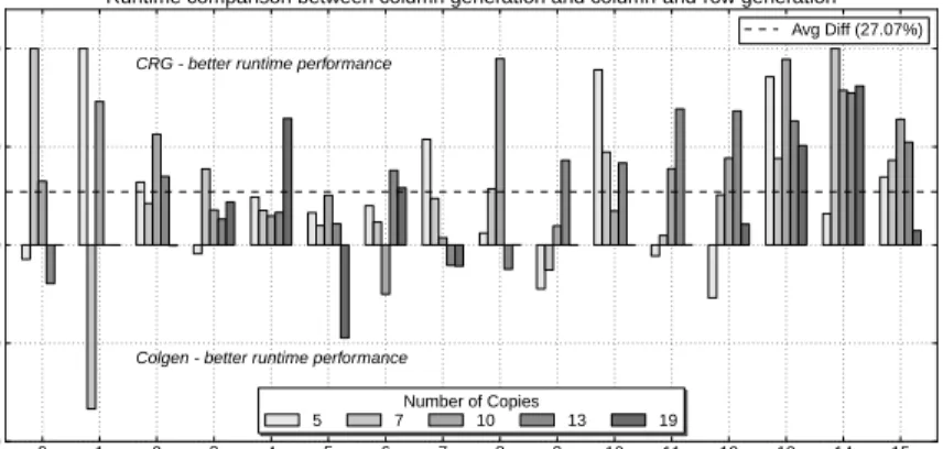
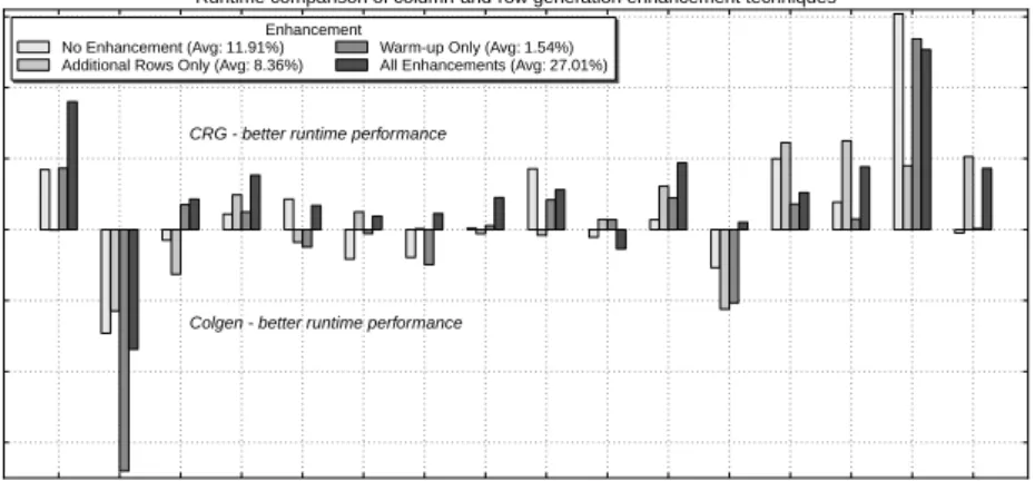
Example applications of this solution approach are Zak [42] with the multi-stage cutting stock problem, Avella et al. [7] solving a time-constrained routing problem and Muter et al. [27] to solve a robust crew pairing problem. While these papers present implementations of column-and-row generation there is little evaluation against a standard column generation approach. A contribution of this paper is such an evaluation using the integrated airline recovery problem as an example. The integrated airline recovery problem is a large-scale, real-world optimisation problem that provides an appropriate test bed for the column-and-row generation framework. This evaluation will demonstrate the improvement in solution runtime and quality compared to column generation and identify a number of enhancements that contribute to the general column-and-row generation approach. The enhancement techniques identified are a variation on the number of rows added in the row generation procedure and a row warm-up process. Since the framework developed in this paper extends Muteret al.[26], the evaluation performed demonstrates the strength of the framework by [26]
The various implementations of column-and-row generation have very little discussion regarding row generation in the branch-and-price algorithm. For example, Zak [42] only solves the LP of the multi-stage cutting stock problem using column-and-row generation, this is also the case in Wang and Tang [38] for the batch machine scheduling problem. Also, Frangioni and Gendron [17, 18] solve the multicommodity capacitated network design problem with column-and-row generation at the root node and then employ branch-and-bound to identify integer solutions. Sadykov and Vanderbeck [33] mention the use of their approach in a branch-and-price algorithm, however no details are provided regarding the implementation. Finally, the framework by Muteret al.[26] is designed to solve large-scale linear programming problems, as such the integration with a branch-and-price algorithm is not considered. A contribution of this paper is a clear description of the application of row generation in a branch-and-price algorithm.
1.3
Outline of paper
This paper presents an integrated airline recovery problem, integrating the schedule, aircraft and crew recovery stages. The integrated airline recovery problem is used in this paper as a real-world example to demonstrate the ability of column-and-row generation to improve solution runtimes and quality. The master problem for the integrated recovery problem is presented in Section 2, which is solved using column generation to provide benchmark results. A general framework for the column-and-row generation solution approach is presented in Section 3. The application of column generation and column-and-row generation is discussed in Section 4, including the description of enhancement techniques. To demonstrate the benefits of solving the integrated recovery problem by column-and-row generation, a comparison with the results produced using column generation is made in both solution quality and runtime. These results are presented in Section 5. The conclusions provided in Section 6 aim to present the technique of column-and-row generation as an alternative solution method for integrated airline and transportation problems.
2 INTEGRATED RECOVERY PROBLEM - IRP 6
2
Integrated Recovery Problem - IRP
The integrated recovery problem (IRP) attempts to minimise the costs associated with flight delays and cancellations and the additional cost of crew following a schedule disruption. This problem is formulated to integrate the schedule, aircraft and crew recovery problems. The link between the aircraft and crew recovery problems in the IRP is provided by the flight cancellation and delay decisions and specific flights allocated to each aircraft and crew.
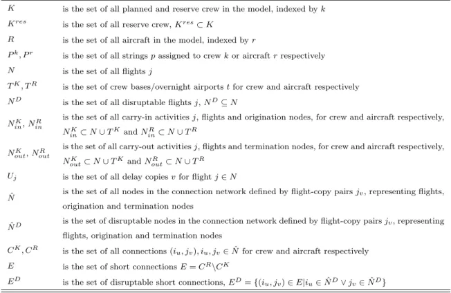
The notation used to describe the IRP is introduced in Tables 1 and 2. For this problem, the set of all crew is given byK, indexed byk, and the set of all aircraft is given byR, indexed byr. The set Kalso includes all available reserve crew Kres. As an extension on current techniques, the solution approach for the IRP demonstrates an efficient algorithm that includes all crew and aircraft, as defined byKand
Rrespectively. Using all crew and aircraft allows the optimal allocation of all available resources.
K is the set of all planned and reserve crew in the model, indexed byk Kres
is the set of all reserve crew,Kres⊂K
R is the set of all aircraft in the model, indexed byr Pk, Pr
is the set of all stringspassigned to crewkor aircraftrrespectively
N is the set of all flightsj
TK, TR is the set of crew bases/overnight airportstfor crew and aircraft respectively
ND
is the set of all disruptable flightsj,ND⊆N
NK
in,NinR
is the set of all carry-in activitiesj, flights and origination nodes, for crew and aircraft respectively,
NK
in⊂N∪TKandNinR⊂N∪TR
NK
out,NoutR
is the set of all carry-out activitiesj, flights and termination nodes, for crew and aircraft respectively,
NK
out⊂N∪TK andNoutR ⊂N∪TR Uj is the set of all delay copiesvfor flightj∈N
ˆ
N is the set of all nodes in the connection network defined by flight-copy pairsjv, representing flights,
origination and termination nodes ˆ
ND is the set of disruptable nodes in the connection network defined by flight-copy pairsjv, representing
flights, origination and termination nodes
CK, CR is the set of all connections (i
u, jv), iu, jv∈Nˆ for crew and aircraft respectively E is the set of short connectionsE=CR\CK
ED is the set of disruptable short connections,ED={(i
u, jv)∈E|iu∈NˆD∨jv∈NˆD}
Table 1: Sets used in the IRP.
2.1
Recovery flight schedule and connection network
A single day flight schedule is used to describe and evaluate the IRP, with the set of flights in the schedule given by N. A critical aspect of the model is the use of a recovery window that specifies the time allocated to return the operations back to plan. The recovery window is described as a time period which defines the set of disruptable flightsND⊆N. The setNDcontains all flights that are primarily
2 INTEGRATED RECOVERY PROBLEM - IRP 7
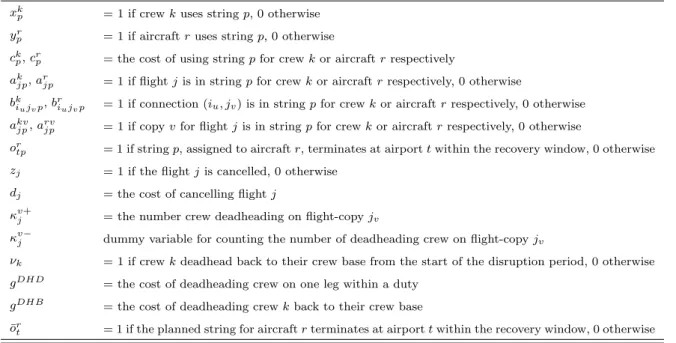
xk
p = 1 if crewkuses stringp, 0 otherwise yr
p = 1 if aircraftruses stringp, 0 otherwise ck
p,crp = the cost of using stringpfor crewkor aircraftrrespectively ak
jp,arjp = 1 if flightjis in stringpfor crewkor aircraftrrespectively, 0 otherwise bk
iujvp,b r
iujvp = 1 if connection (iu, jv) is in stringpfor crewkor aircraftrrespectively, 0 otherwise akv
jp,arvjp = 1 if copyvfor flightjis in stringpfor crewkor aircraftrrespectively, 0 otherwise or
tp = 1 if stringp, assigned to aircraftr, terminates at airporttwithin the recovery window, 0 otherwise zj = 1 if the flightjis cancelled, 0 otherwise
dj = the cost of cancelling flightj κv+
j = the number crew deadheading on flight-copyjv κv−
j dummy variable for counting the number of deadheading crew on flight-copyjv
νk = 1 if crewkdeadhead back to their crew base from the start of the disruption period, 0 otherwise
gDHD
= the cost of deadheading crew on one leg within a duty
gDHB = the cost of deadheading crewkback to their crew base
¯
or
t = 1 if the planned string for aircraftrterminates at airporttwithin the recovery window, 0 otherwise
Table 2: Variables used in the IRP.
affected by the disruption and those that depart after the disruption occurs, but before the end of the specified time window.
Restricting the flights included in the IRP using a recovery window requires the activities performed by crew and aircraft before and after this window to be fixed. This introduces the concepts of carry-in and carry-out activities. A carry-in activity is a flight or origination airport that is assigned to a crew or aircraft directly preceding the disruption, contained in the sets NK
in andN R
in respectively. A carry-out activity is a flight or termination airport assigned to a crew or aircraft immediately after the end of the recovery window, contained in the sets NK
out and NoutR respectively. Now, the carry-in activity describes an origination airport when a planned crew duty or aircraft routing begins after the start of the disruptive event. In a similar manner, if a planned crew duty or aircraft routing concludes before the end of the recovery window, the carry-out activity is defined as the terminating airport.
To achieve an efficient solution approach for the IRP, the recovery policy of flight delays is imple-mented using flight copies. The flight copies technique involves the multiple duplication of each flight contained inN with each copy assigned a progressively later departure time. For each flightj∈N the set of discrete copies is given byUj, and a flight-copy pair is described byjv, wherev∈Uj. Since the set of all flightsN is partitioned into disruptable and non-disruptable sets, the set of discrete flight copies requires a different definition for each partition. As such, for all non-disruptable flights, j ∈ N\ND, only one copy is included to represent the original scheduled departure, i.e. Uj ={0}. Further, for all disruptable flights,j∈ND, the set of flight copiesU
j contains a copy representing the original departure time and at least one additional copy to represent some delay on that flight. It is important to note that the nodes representing origination and termination airports are treated as non-disruptable flights. This
2 INTEGRATED RECOVERY PROBLEM - IRP 8
definition is made for convenience in discussing carry-in and carry-out activities.
The connection network used for this model is described using the flight-copy representation for each node in the network. The set of all nodes is represented by ˆN = {jv|j ∈ N ∧v ∈ Uj}, detailing all flight-copy pairs that exist for each disruptable and non-disruptable flight. Using the same notation, the set of all disruptable nodes is given by ˆND ={j
v|j ∈ND∧v ∈Uj}. The connection network for this problem is defined by a set of nodes, representing flight-copy pairs, and a set of arcs as connections between the nodes. A connection between two flight-copy pairs (iu, jv), iu, jv ∈Nˆ is feasible if i) the destination of flightiis the same as the origin of flightj and ii) departure of flight-copyjv occurs after a specified amount of time following the arrival of flight-copy iu. All feasible connections for crew are contained in the setCK and require aminimum sit time between the arrival ofi
uand the departure of
jv. Similarly, all feasible connections for aircraft contained inCRrequire aminimum turn time between the connecting flights.
2.2
Aircraft routes and crew duties
The modelling approach for the IRP is based upon the string formulation introduced by Barnhart et al.[9]. In the IRP, a flight string is defined as a set of connected flights from a carry-in to a carry-out activity. Using the flight-copy notation of each node for this model, any reference to flight j without specifying a copyvcollectively states all flight-copy pairs associated with that flight. So, the parameters
ak
jpandarjp specify whether flightj, representing any flight-copy pairjv, v∈Uj, is included on stringp for crewk and aircraftrrespectively. A flight string will either terminate within the recovery window, by ending at a crew base or aircraft overnight port, or will terminate at a carry-out flight. If the flight string assigned to an aircraft terminates within the recovery window, the parameter or
tp describes the terminating airporttfor aircraftr. Flight cancellations are implemented as a recovery policy for the IRP, so the flow balance of the original schedule is not maintained. To ensure enough aircraft are positioned at each airporttto operate the schedule for the following day, the minimum number of required aircraft must be specified. Now, the number of planned aircraft strings terminating at end-of-day locations within the recovery period is given byP
r∈Ro¯ r
t,∀t∈T, where ¯ort indicates that aircraft rterminates at airport t. Therefore this expression defines the minimum number of aircraft required to terminate at each end-of-day locationtwithin the recovery window for the IRP.
Within the set of all aircraft connections,CR, it is common to have connection times less than the minimum sit time for crew. These connections are called short connections, and it is permissible for crew to operate the two flights in succession, as defined by this connection, only if a single aircraft also operates the same two flights. The set of all short connections are contained in E = CR\CK, and the subset of short connections that include flight-copy pairs in ˆND are contained in the set ED. If a flight string includes two flight-copy pairs that form a short connection, the parametersbk
iujvp andb
r iujvp
2 INTEGRATED RECOVERY PROBLEM - IRP 9
2.2.1 Legality of crew duties
There a numerous rules that dictate the construction of feasible flight strings for crew that must be strictly adhered to in the recovery problem. A good review of the crew scheduling problem is presented by Barnhart et al. [10], discussing the numerous crew rules. There are rules that are specific to the construction of duties, pairings and schedules, however for a single day schedule, which is used for the IRP, the most important rules that must be considered are the crew duty rules.
The origination and termination locations are critical in the construction of legal crew duties. Each crew is employed at one of many crew bases throughout the network, so ideally a duty is constructed to start and end at the same crew base. Unfortunately, the design of the flight schedule does not permit all crew duties to terminate at their respective crew base, requiring an overnight stay at a permissible airport. This rule is modelled in the IRP and if a crew duty originates from a permissible overnight airport, it must terminate the required crew base.
The number of hours that a crew duty spans is crucial in managing the effects of fatigue. There are two rules related to working hours modelled in the IRP, a maximum number of flying hours and limit on the duration of the crew duty, which are set of 8 and 13 hours respectively. These are the most important duty rules related to working hours, and are strictly adhered to in the IRP. Another important, but complicated, rule is the 8-in-24 rule that requires crew to receive additional rest of more that 8 hours flying is performed in a 24 hour period [10]. This rule must be considered in the construction of crew pairings, however it may be reviewed in the recovery of crew duties. By ensuring that crew only perform 8 hours flying in a single day and given that individual crew members have planned work starting times, the 8-in-24 rule will not be violated in most cases. In the event that this rule is violated by the solution to the IRP, further adjustment can be made to the recovered duties at the end of the day to provide an adequate amount of rest.
It is important to note that prior to a disruption crew may have performed part of a duty, consuming allowable flying and working hours. The personalised schedules are respected in the recovery of crew duties by originating each duty from a carry-in location and accounting for the workinghistory prior to the disruption. This ensures that the recovered crew duties, including the flights performed prior to the disruption, respect the crew duty rules.
2.3
Recovery policies
The set of recovery policies implemented for the IRP include the generation of new aircraft routes and crew duties, crew deadheading (transportation of crew as passengers), the use of reserve crew, and flight delays and cancellations. In the column generation algorithm, feasible crew duties and aircraft routes are generated for each crew and aircraft contained in K and R respectively. The length of delay that is required on each flight is determined in the generation of these new flight strings by the selection of
2 INTEGRATED RECOVERY PROBLEM - IRP 10
flight-copy pairs. The parametersakv
jpandarvjpdescribe the length of delay, as specified by copyv, selected for flight j on string pfor the crew and aircraft respectively. The IRP also allows for the cancellation of any flight that can not be covered by both crew and aircraft. Flight cancellations are defined in the IRP through the use of the variableszj, which equal 1 to indicate flightj is cancelled at a cost ofdj.
Following a disruption, it is not always possible for every crew member to operate the originally planned flight strings as expected. Hence, the crew specific recovery policies of deadheading and the use of reserve crew are employed. Crew deadheading transports crew as passengers to continue the operation of disrupted flight strings. Two different types of deadheading are implemented in the IRP, deadheading within a duty and deadheading back to base. The variablesκv+
j are introduced to count the number of crew that deadhead within a duty on flight-copyjv. In addition, the dummy variables κv−j are required to ensure that the number of crew deadheading on flight-copyjvis one less than the total number of crew assigned to that flight-copy. The cost of crew deadheading within a duty is given bygDHD. Alternatively, the variablesνk indicate whether crewkdeadhead to their crew base immediately following the start of the disruption at a cost of gDHB. As a result of recovery actions, it is not guaranteed that the set of originally planned crew are able to operate the recovered schedule. Hence, reserve crew are employed to operate crew duties from each crew base. Reserve crew are a limited, costly resource, as such their use in the solution to the IRP is minimised by the addition of a penalty to the costck
p for each duty they perform.
The integrated recovery problem is presented in a compact formulation with variables xk
p for crew andyr
p for aircraft representing feasible flight strings. The full description of this problem is presented below,
2 INTEGRATED RECOVERY PROBLEM - IRP 11 (IRP) min X k∈K X p∈Pk ck px k p+ X j∈ND X v∈Uj gDHDκv+ j + X k∈K gDHBν k+ X r∈R X p∈Pr cr py r p+ X j∈ND djzj, (1) s.t. X k∈K X p∈Pk ak jpx k p− X v∈Uj κv+ j +zj = 1 ∀j∈ND, (2) X k∈K X p∈Pk akjpx k p = 1 ∀j∈N K out, (3) X r∈R X p∈Pr arjpy r p+zj = 1 ∀j∈ND, (4) X r∈R X p∈Pr ar jpy r p= 1 ∀j∈N R out, (5) X r∈R X p∈Pr or tpy r p≥ X r∈R ¯ or t ∀t∈T, (6) X k∈K X p∈Pk akv jpx k p−κ v+ j +κ v− j = 1 ∀j∈N D,∀v∈U j, (7) X k∈K X p∈Pk bkiujvpx k p− X r∈R X p∈Pr briujvpy r p≤0 ∀(iu, jv)∈ED, (8) X k∈K X p∈Pk akv jpxkp−κ v+ j − X r∈R X p∈Pr arv jpyrp= 0 ∀j∈ND,∀v∈Uj, (9) X p∈Pk xk p+νk = 1 ∀k∈K\Kres, (10) X p∈Pk xk p ≤1 ∀k∈K res, (11) X p∈Pr yrp≤1 ∀r∈R, (12) xkp ∈ {0,1}, ∀k∈K,∀p∈P k , ypr∈ {0,1}, ∀r∈R,∀p∈P r , (13) zj∈ {0,1}, ∀j∈ND, νk ∈ {0,1}, ∀k∈K, (14) κv+ j ≥0, κ v− j ≥0, ∀j∈N D,∀v∈U j. (15)
The IRP is defined by equations (1)-(14) with the objective to minimise the cost of recovery for aircraft and crew. The recovery costs include the cost of flight delays and cancellations, reserve crew, additional crew duty costs and the cost of crew deadheading.
The coverage of flights within the recovery window by the crew and aircraft is enforced by constraints (2) and (4). Additionally, the constraints (3) and (5) ensure that each carry-out flight is serviced by crew and aircraft in the recovered solution. Respecting the carry-out flight coverage ensures that the solution to the IRP positions the crew and aircraft to continue the activities as planned, following the end of the recovery window.
This problem is solved for a single day schedule, so the aircraft are required to be positioned at airports to maintain flow balance for the following days operations. Since all recovery actions occur within the recovery window, the positioning of the aircraft must be considered before the conclusion of
2 INTEGRATED RECOVERY PROBLEM - IRP 12
this window. Two cases can occur in the recovery of aircraft; either i) an aircraft is assigned a carry-out flight, allowing it to follow a planned routing to an end-of-day location, or ii) the recovered flight route terminates within the recovery window requiring an end-of-day location to be specified. The minimum number of aircraft required to terminate at each end-of-day location within the recovery window is enforced through constraints (6).
The recovery policy of crew deadheading within a duty is implemented through the surplus crew count constraints (7). This set of constraints ensure that crew deadheading is only permitted on flight-copy pairs that are operated by at least one crew.
In the IRP, the integration between the crew and aircraft variables is described by the short connection and delay consistency constraints, equations (8) and (9) respectively. The short connection constraints (8) ensure that crew are only permitted to use connection (iu, jv)∈ED only if an aircraft is also using the same connection. The delay consistency constraints (9) ensure that the length of delay on any flight in a feasible aircraft recovery solution is identical for the crew recovery solution, and vice versa. Since there exists one delay consistency constraint for each flight-copy pair, this set of constraints grows very quickly with an increase in the number of copies. It is on this set of constraints that the row generation procedure is implemented to improve the solution runtime.
The number of crew and aircraft operating the recovered schedule is based upon the originally planned duties and routings. Each crew that is assigned a duty from the planning stage must also be assigned a duty in the IRP or deadheaded back to base, captured by constraints (10). This is not true for the reserve crew since they former is not required to perform any duties during recovery, which is captured by the inequality in constraints (11). Similar for crew, each aircraft that is assigned a flight route in the planned solution must be assigned a flight route in recovery, which is given by (12)
It is common practice in both the sequential stage and integrated recovery problems to select a subset of crew, aircraft and flights to reduce the problem size and improve solution runtimes. To improve the computational performance of the IRP, the concept of a recovery window has been used to reduce the number of flights included in the optimisation problem. While this provides an upper bound on the optimal recovery cost, it is believed that this approach is realistic and consistent with a common objective to quickly return operations to plan. Returning operations to plan is a consequence of the carry-out activity coverage at the conclusion of the recovery window. Hence, the shorter the recovery window, the quicker operations are returned to plan. To ensure that all reassignment and rerouting options are available, the full set of crew and aircraft are used in the IRP. The selection of all crew and aircraft for this problem demonstrates that fast solution algorithms are possible on larger data sets using sophisticated solution techniques.
3 COLUMN-AND-ROW GENERATION 13
3
Column-and-Row Generation
This paper demonstrates the improvements in the solution runtimes and quality for the IRP achieved by employing column-and-row generation. As discussed in Section 1.2, there have been a number of generic column-and-row generation approaches that have been developed [18,26,33]. Unfortunately, these generic approaches do not directly apply to the IRP, as such an alternative framework will be presented in the following sections. The framework developed in this paper is an extension of Muter et al. [26] and is presented as an alternative solution approach to Benders’ decomposition. The key contributions of this framework are i) the extension of [26] to consider multiple sets of secondary variables and linking constraints, ii) the application of column-and-row generation to a problem structure that is commonly solved by Benders’ decomposition, and iii) the explicit evaluation against a standard column generation approach, identifying various enhancement techniques.
3.1
Features of the Column-and-Row Generation Framework
The solution approach presented by Muter et al.[26] involves defining two restrictions on the original problem, the restricted master problem (RMP) and the short restricted master problem (SRMP). The RMP is constructed to contain all constraints from the original problem but with only a subset of all possible variables. The SRMP describes a further restriction on the original problem, containing a subset of all variablesand constraints that form the RMP.
Both the RMP and SRMP are solved by column generation and the identical subproblems are used in the solution process for the two problems. However, the SRMP is formed by eliminating structural constraints from the RMP, so variable fixings in the column generation subproblems are used to restrict the set of all possible columns. By applying the variable fixing to the column generation subproblem, all feasible solutions to the SRMP are feasible for the RMP and the original problem.
Column-and-row generation is a solution approach proposed to solve large-scale linear programs. The implementation of column-and-row generation in a branch-and-price framework to solve mixed-integer programs has not been previously published. As a contribution of this paper, an efficient method for applying column-and-row generation at each node in the branch-and-bound tree is explicitly discussed. The critical aspects of the column-and-row generation procedure are the formulation of the RMP and SRMP, and the method used to calculate an optimal dual solution to identify favourable rows. These two features will be discussed in Sections 3.1.1 and 3.1.2 respectively. Finally, a general algorithm for the row generation procedure will be presented in Section 3.1.3.
3.1.1 Formulation of the restricted problems
To provide an overview of column-and-row generation, the key features will be discussed with respect to a generic problem. The example problem is formulated with a single set of primary variables and
3 COLUMN-AND-ROW GENERATION 14
multiple sets of secondary variables. In the problem descriptionxis used to represent a single vector of primary variables, and each vector of secondary variables is given by yi, i∈ {1,2, . . . , n}. The multiple sets of secondary variables considered in this framework extends the generic framework presented by Muteret al.[26].
This section focuses on problems solved by column generation, as such it is assumed that vectorsx
and yi contain only a subset of all possible variables from the original problem. The structure of the original problem, and by extension the RMP, contains a set of constraints related to eachxandyi,Axand
Ai respectively, with a set of linking constraintsAiL
x andAiLy betweenxandyi. The rows representing the linking constraints are dynamically generated using the row generation procedure developed in this section.
To construct the SRMP, it is necessary to redefine the variable vectors and constraint matrices used to describe the RMP. Initially, a subset of linking constraints are eliminated from the RMP, which involves removing rows fromAiL
x andA iL
y , resulting in the constraint matrices ¯A iL x and ¯A
iL
y respectively. As stated previously, the elimination of rows from the RMP is coupled with the fixing of variables in the column generation subproblem. This is required to prohibit the generation of columns with non-zero elements in the eliminated rows. Consequently, the set of all possible variables that can be generated for the SRMP is reduced, therefore the vectors ¯x⊂ xand ¯yi ⊂yi are defined. While all rows in the matricesAx andAi are still present in the formulation of the SRMP, the restriction on the possible set of variables requires the elimination of columns, hence the matrices ¯Axand ¯Ai are defined.
The matrix representation of the RMP and SRMP is given by,
RMP SRMP min cxx+X i ciyi, (16) s.t. Axx=b, (17) Aiyi =bi ∀i, (18) AiL x x−A iL y y i= 0 ∀i, (19) x≥0, yi≥0. (20) min ¯cxx¯+X i ¯ ciy¯i, (21) s.t. A¯xx¯=b, (22) ¯ Aiy¯i=bi ∀i, (23) ¯ AiL x x¯−A¯ iL y y¯ i= 0 ∀i, (24) ¯ x≥0, y¯i≥0. (25)
3.1.2 Calculation of dual solutions
To demonstrate the correctness of the column-and-row generation approach described here, an additional problem is introduced, the RMP′. This problem is formulated with all constraints from the RMP, but only a subset of all possible variables. Thus, the formulation of the RMP′ is identical to the RMP at an intermediate stage of the column generation solution process.
To describe the RMP′, the matrices ˜AiL
y are introduced to contain all rows eliminated from AiLy to construct the SRMP. Additionally, a set of dummy variables ˜yi are created such that eachy ∈ y˜i has
3 COLUMN-AND-ROW GENERATION 15
a non-zero element in only one row of ˜AiL
y . This is an important condition on the construction of ˜yi that is exploited in Theorem 3.1.1. The dummy variables contained in ˜yi also have non-zero elements in the rows of (18), thus the matrices ˜Ai must be introduced. Therefore, the matrix representation of the RMP′ is given by,
(RMP′) min c¯x¯+X i {¯ciy¯i+ ˜ciy˜i}, (26) s.t. A¯x¯=b, (27) ¯ Aiy¯i+ ˜Aiy˜i=bi ∀i, (28) ¯ AiL x x¯−A¯iLy y¯i= 0 ∀i, (29) −A˜iL y y˜ i= 0 ∀i, (30) ¯ x≥0, y¯i≥0, y˜i≥0. (31)
For each row in equations (27)-(30) there is an equivalent row in equations (17)-(19). It is assumed that in this formulation the optimal solution to the RMP′is not the optimal solution to the original problem. Thus, additional columns with a negative reduced cost can be found by solving the column generation subproblems for the primary and secondary variables.
By construction, an optimal primal solution to the SRMP is a feasible solution to the RMP′. The following lemma will prove that this feasible primal solution to the RMP′ is optimal.
Lemma 3.1.1. The optimal primal solution to the SRMP is an optimal primal solution to the RMP′.
Proof. The constraints (30) force the variables ˜yi to be zero in any feasible solution of the RMP′. As such, the optimal primal solution to the RMP′can be found by eliminating constraints (30) and solving this problem with the variables ˜yi fixed to zero. Solving this modified form of the RMP′ is equivalent to solving the SRMP.
There are two major steps in the procedure to calculate an optimal dual solution for the RMP′ using the solution to the SRMP. Firstly, the constraints (22)-(24) in the SRMP are identical to the constraints (27)-(29), therefore the solutions to the related dual variables can be simply equated. The second step involves finding the solutions for the dual variables related to the rows in (30), which are the constraints eliminated to form the SRMP. This involves solving the column generation subproblems for the secondary variables to accurately calculate the values of these dual variables.
Additional notation is required to describe the calculation of the dual variables for the rows eliminated to form the SRMP. An index set Φi is defined to reference each row u in the constraint matrix AiL
y . Extending this notation, the index set for the rows included in the SRMP is given by ¯Φiand all eliminated rows are contained in Φi\Φi. Finally, the dual variables for each row in¯ AiL
y is given byθi ={θiu|u∈Φi}. This notation conveniently describes the rows which are eliminated or contained in the SRMP and the
3 COLUMN-AND-ROW GENERATION 16
dual values which must be computed. The value of θi
u is calculated from the minimum reduced cost ˆci for a variable with a non-zero entry in rowuof matrix ˜AiL
y . This is achieved by executing Algorithm 1.
Algorithm 1Computing a feasible dual solution
1: Assume that θi
u = 0 and force all feasible solutions to the column generation subproblem for the secondary variables ito have a 1 in rowuof ˜AiL
y and 0 in all rowsv∈Φi\Φi¯ , v6=u.
2: Solve the column generation subproblem to identify variable ˆy that has the minimum reduced cost
ˆ
ci.
3: Setθi u=−ˆci.
This calculation procedure relies on the structure of the RMP′and the form of the dummy variables that populate the rows u∈Φi\Φi. The reasoning provided here draws upon the discussion presented¯ in the column-and-row generation framework by Muter et al. [26]. For ˆy, found by Algorithm 1, to be eligible to enter the basis of the RMP′ implies that ˆci <0. Since ˆy has a non-zero element in the rows of ˜AiL
y , the construction of the RMP′ forces ˆy = 0 upon addition of this column, resulting in a degenerate simplex iteration. To avoid this situation, it is assumed that the minimum reduced cost for all variables found using Algorithm 1 is at least zero. This requirement ensures that the dual solutions that are computed forθi are feasible for the RMP′. The following theorem will prove the feasibility of the computed values forθi and that the resulting feasible dual solution is also optimal.
Theorem 3.1.1. The dual solutions computed forθi forms an optimal dual solution to the RMP′.
Proof. The first step of this proof is to show that the solutions calculated for the dual variablesθi using Algorithm 1 are feasible for the RMP′. For this proof the variable ¯θi
u is assumed to have a value that satisfies all dual constraints of the RMP′. Additionally, the reduced cost of variable y∈y˜i is given by ¯
ci y.
Algorithm 1 solves the column generation subproblem for the secondary variablesito identify ˆy that has the minimum reduced cost ˆci, assuming θi
u = 0. Comparing ˆy with the variables currently in the RMP′, there are two possible outcomes:
i) There exists a columny∈y˜i identical to ˆy. Sinceyis identical to ˆy, ˆci= ¯ci
y−θ¯iu. In Algorithm 1, the value ofθi
uis set to−cˆi, hence ¯ciy−θ¯ui +θui = 0. Therefore, settingθui =−ˆciensures dual feasibility. ii) There exists a column y ∈y˜i that has a non-zero element in row uof ˜AiL
y but is not identical to ˆy. This implies that the variableθi
u exists in at least one dual constraint. Lets assume that setting
θi
u=−ˆci violates a constraint in the dual of the RMP′. This implies that ¯ciy calculated usingθiu=−ˆci in place of ¯θi
u is negative, i.e. ¯ciy−θ¯ui +θui < 0. Since ˆci+θiu = 0, then ˆci > c¯iy−θ¯u. Now, stepi 2 of Algorithm 1 identifies ˆy that has the minimum reduced cost, so ˆci > ¯ci
y−θ¯ui is a contradiction. Therefore, ¯ci
y−θ¯iu+θui ≥0 must be true, hence the computed value forθiusatisfies all dual constraints. The first step of this proof has established that the dual solutions calculated forθi using Algorithm 1 are feasible for the RMP′. Therefore, the calculated values forθican be used as the dual solutions for
3 COLUMN-AND-ROW GENERATION 17
the constraints (30). A feasible dual solution for the RMP′ is then simply constructed by equating the solutions to the dual variables representing constraints (27)-(29) to the dual solutions of the SRMP.
The second step proves that the feasible dual solution constructed for the RMP′ is also optimal. Firstly, it is stated in Lemma 3.1.1 that the optimal primal solution to the SRMP is also optimal for the RMP′. In addition, the solutions to the dual variables representing constraints (27)-(29) are equated to the dual solutions of the SRMP. Since the right hand side of the constraints represented by equations (30) are zero, the value of the respective dual variables do not affect the optimal objective function value. It follows that the dual objective function value for the RMP′ is identical to the dual objective function value of the SRMP. Given that the dual objective function value of the SRMP is equal to the primal objective values of the SRMP and RMP′, then primal and dual objective values for the RMP′ are equal. Therefore, the feasible dual solution constructed for the RMP′ is optimal.
3.1.3 Row generation algorithm
Using the optimal dual solution to the RMP′, the row generation algorithm is executed to identify rows to update the SRMP. This procedure involves solving the column generation subproblem for the primary variables to find negative reduced cost columns feasible for the RMP′. It is likely, due to the eliminated constraints, that the columns identified during this procedure are infeasible for the SRMP. Such columns are identified by displaying at least one non-zero element in the rows contained in Φi\Φi.¯ If columns infeasible for the SRMP are found, thenumust be added to ¯Φi and the related row to the SRMP. Consequently, the SRMP grows vertically and horizontally with the addition of rows and columns respectively. The row generation procedure is detailed in Algorithm 2.
Algorithm 2Row generation algorithm
Require: An optimal solution to the SRMP.
1: Set the dual values for rows (27)-(29) to the dual solutions for the rows (22)-(24).
2: for allsecondary variable setsido
3: for allrowsucontained in ˜AiL y do
4: Execute Algorithm 1 to compute the value ofθiu.
5: end for
6: end for
7: By Theorem 3.1.1 an optimal dual solution for the RMP′ has been computed.
8: Solve the column generation subproblem for the primary variables to identify variables feasible for
the RMP′.
9: if a negative reduced cost column has at least one non-zero entry in the rows of ˜AiL y then
10: add the rows with non-zero entries in ˜AiL y to ¯A
iL y .
4 APPLYING THE COLUMN-AND-ROW GENERATION FRAMEWORK 18
The column-and-row generation solution approach terminates when no favourable rows are identified by Algorithm 2. This is consistent with the termination condition of the standard column generation approach, terminating when no columns with a negative reduced cost for the RMP are found. Since an optimal dual solution is calculated for the RMP′, the column generation subproblem for the primary variables accurately evaluates the minimum reduced cost. Therefore, if no negative reduced cost columns are found for the RMP′, then the solution to the RMP′, and the SRMP, is optimal for the original problem.
3.2
Column-and-Row Generation Solution Algorithm
The column-and-row generation solution algorithm implemented in this paper is developed by combining the fundamental features of the approach developed throughout Section 3.1. The first stage of the solution algorithm involves the formulation of the SRMP, which is detailed in Section 3.1.1. Using the solution to the SRMP, Section 3.1.2 details the calculation procedure that is required to form an optimal dual solution for the RMP′. The final step in the column-and-row generation solution algorithm, described in Section 3.1.3, executes Algorithm 2 to identify favourable rows for the SRMP. The complete column-and-row generation solution algorithm is given by Algorithm 3.
Algorithm 3Column-and-row generation algorithm
1: Eliminate columns from the original problem to form the RMP.
2: Eliminate rows (and subsequently columns) from the RMP to form the SRMP.
3: repeat
4: Solve the SRMP by column generation to optimality.
5: Use Algorithm 2 to compute the optimal dual solution to the RMP′ and identify any favourable rows.
6: untilno rows are added to ¯AiL
y in Algorithm 2
7: The solution to the SRMP is the optimal solution to the original problems
4
Applying the Column-and-Row Generation Framework
The framework presented in Section 3 describes the features of column-and-row generation that extend the standard column generation approach. Column generation is a critical aspect of column-and-row generation, as such its implementation for the IRP will be discussed in Section 4.1. This will be followed by a review of the features presented in Section 3.1, detailing the application to the IRP in Section 4.2.
4 APPLYING THE COLUMN-AND-ROW GENERATION FRAMEWORK 19
4.1
Column Generation
The formulation of the IRP presents two sets of variables for which column generation is applied. These variables are related to crew duties and aircraft routes, which are defined as flight strings. While each of the variables types have similar structures, there are specific rules governing their generation. Hence, two individual column generation subproblems are required in the solution process. In this section, the column generation subproblem for each variable type is described, including the relevant solution methods.
In the column generation procedure, a restricted master problem (RMPIRP) is defined by including only a subset of all possible columns, ¯Pk ⊆ Pk and ¯Pr ⊆Pr, and is solved to find the optimal dual solution. The dual variablesαK ={αK
j ,∀j ∈N D∪NK out}andα R={αR j,∀j∈N D∪NR
out} are defined for the flight coverage constraints (2)-(3) and (4)-(5), respectively. The dual variables for the aircraft end-of-day location constraints (6) are defined by ǫ={ǫt,∀t∈T}. The dual variables for the surplus crew count constraints (7) are given byη={ηv
j,∀j∈ND,∀v∈Uj}. For the short connection constraints (8) and the delay consistency constraints (9), the dual variables are given by ρ ={ρij,∀(i, j) ∈ ED} and γ = {γv
j,∀j ∈ ND,∀v ∈ Uj}, respectively. Finally, the dual variables δK = {δk,∀k ∈ K} and
δR = {δr,∀r ∈ R} are defined for the crew and aircraft assignment constraints, (10)-(11) and (12), respectively. Using the set of optimal dual solutions, the column generation subproblems for crew and aircraft are solved to identify negative reduced cost columns to add to the sets ¯Pk and ¯Pr.
4.1.1 Crew Pairing Subproblem
The crew duty subproblem (PSPk) is solved as a shortest path problem with one source node and multiple sink nodes. The general form of the PSPk is given by,
ˆ ck p = min p∈Pk ( RecDutyCost(k)− X j∈ND∪NK out αjakjp− X (iu,jv)∈ED ρiujvb k iujvp− X j∈ND X v∈Uj n ηv j+γ v j o akv jp−δ k ) (32) The set Pk is defined as the feasible region to a network flow problem, as such the PSPk is solved as a resource constrained shortest path problem (RCSPP). The important features of the RCSPP used to solve the PSPk is the origination of each crew k from a unique carry-in activity and the termination at any carry-out activity. In addition, the crew duty rules considered in this paper are the maximum number of flying and working hours, which are set at 8 and 13 respectively. In the column generation and column-and-row generation solution approaches the PSPkis solve once for eachk∈Kin each iteration. In the objective function of (32), the complex cost structure used for crew remuneration is denoted by
RecDutyCost(k), which defines the additional crew cost resulting from recovery actions. The recovery
crew costRecDutyCost(k) is amaxfunction related to the number of flying hours,f ly(k), the number of working hours, elapse(k), a minimum number of guaranteed hours, minGuar, and the originally
4 APPLYING THE COLUMN-AND-ROW GENERATION FRAMEWORK 20
planned duty cost,OrigDutyCost(k). As such, the expression for the cost of a duty in the IRP is given by
RecDutyCost(k) = max{0,max{f ly(k), fd·elapse(k), minGuar} −OrigDutyCost(k)}, (33)
whereminGuaris set at 6 hours [10] andfdis a fraction which is airline specific and is set atfd= 5/8 [10]. In consideration to the resource restrictions and complex cost structure, a multi-label shortest path algorithm is implemented to solve the PSPk. Label l at nodei
u stores the cost of the current shortest path to the node, ˆciul, the number of flying hours, H
1
iul, and the total elapsed hours, H 2
iul. Multiple
labels are necessary to track any suboptimal paths to a node, based on the path length ˆciul, that have
a favourable resource consumption. While it is possible to store every path that arrives at a node, this would be a very inefficient method to track resource consumption. As such, a dominance condition is used to reduce the number of labels stored at each node by eliminating any suboptimal paths demonstrating unfavourable resource consumption.
Definition 4.1.1. (Dominance Condition)
Given two labels at node iu, (ˆciu1, H 1 iu1, H 2 iu1) and (ˆciu2, H 1 iu2, H 2
iu2), that are not equal. Label 1
dominates label 2 if ˆ ciu1≤ˆciu2, H 1 iu1≤H 1 iu2 andH 2 iu1≤H 2 iu2.
Using Definition 4.1.1, the dominance of any new label arriving at a node is evaluated against all currently stored labels. There are three possible outcomes from the comparison between the new label and all currently stored labels. Firstly, if the new label dominates any stored label, the dominated labels are removed from the node. Second, if the new label is dominated by any stored label, then the new label is discarded. Finally, if no dominance is established between the new label and the stored labels, then the new label is added to the list of labels stored at that node. At the sink node, the label that achieves the lowest cost is selected and the resulting path is the minimum reduced cost path.
The connection network described in Section 2 forms an acyclic directed graph. Given this network structure, all the nodes can be listed in a topological order, where node iu is ordered before node jv if
∃(iu, jv)∈CK[4]. Using a topological ordering, the shortest path problem can be solved inO(ml) time in the worst case, wheremis the number of arcs in the acyclic directed graph andlis the maximum number of labels. A pulling algorithm is implemented, which solves the shortest path problem by “pulling” labels from previously processed nodes. Such a pulling algorithm for solving the shortest path problem on an acyclic directed graph is presented in Ahujaet al.[4]. This algorithm can be easily adapted to solve the PSPk with multiple labels.
4 APPLYING THE COLUMN-AND-ROW GENERATION FRAMEWORK 21
4.1.2 Aircraft Routing Subproblem
The column generation subproblem for the aircraft routing variables solves a shortest path problem from an origination location to one of the permissible termination locations. The general form of the column generation subproblem for the aircraft routing variables (PSPr) is given by,
ˆ cr p= min p∈Pr ( cr p− X j∈ND∪NK out αjarjp− X t∈T ǫtortp+ X (iu,jv)∈ED ρiujvb r iujvp+ X j∈ND X v∈Uj γv ja kv jp−δ k ) (34)
Similar to Pk, the set Pr is defined as the feasible region of a network flow problem. However, unlike the PSPk, the PSPrdoes not consider any resources in addition to cost, therefore the column generation subproblem is solved as a standard shortest path problem. The key features of the PSPr is that each flight string must originate from a unique in activity and may terminate at any permissible carry-out activity or overnight airport. In addition, if an aircraft is planned to receive maintenance at the end of the day, the termination locations will ensure that this requirement is met. In the column generation and column-and-row generation solution approaches the PSPr is solve once for each r ∈ R in each iteration.
The PSPr describes a shortest path problem for which a large number of solution algorithms are available. Similar to the connection network for crew, the network for aircraft is an acyclic directed graph. As such, the nodes can be listed in a topological order and an efficient pulling algorithm presented in Ahujaet al.[4] is implemented to solve the PSPr.
In a given iteration of the column generation algorithm, the most negative reduced cost for all aircraft, ˆ
cR
p, can be found by solving the PSPr for each aircraft r and setting ˆcpR = minr∈R{¯crp}. However, all connection costs and dual variables, except for δR = {δr,∀r ∈ R}, included in (34) are aircraft independent. Therefore, by setting δr=δR,∀r∈R, whereδR = maxr∈R{δr} in (34), it is possible to find a lower bound on ˆcR
p, labelled as ¯cRp, by solving the aircraft routing shortest path algorithm only once. The aircraft routing subproblem to be solved only once will be labelled PSPR and will be used as part of the row generation procedure described in Section 4.2.
4.2
Row Generation
An important feature of the IRP is the use of a full set of recovery policies, which includes flight delays. There are a number of different methods that are available to implement flight delays, such as time windows [34] and discrete flight copies [37], each with relative strengths regarding the problem formulation and solution methods. The technique of flight copies has been selected to model delays as a result of its simplicity in implementation for column generation and to fit within the column-and-row generation framework.
4 APPLYING THE COLUMN-AND-ROW GENERATION FRAMEWORK 22
to ensure that the crew duty and the aircraft routing solutions use the same copy (delay) for each flight. The delay consistency constraints, equation (9), capture this, at the expense of adding a large number of constraints to the RMPIRP. Since the optimal variables have non-zero coefficients in only a small subset of the delay consistency constraints, many rows related to these constraints are not required in the RMPIRP.
The implementation of delay copies in the IRP provides alternative flight departure times given by a uniform discretisation of a maximum allowable delay. While this is a popular method of implementation that has been employed by Yan and Young [41], Thengvallet al. [37] and Andersson and Varbrand [5], Bratu and Barnhart [11] state that a number of copies may be dominated by shorter delay options. Further, Petersenet al.[30] suggests the modelling of flight delays by an event-driven approach, linking delays to activities related to each flight. This reduces the size of the recovery problem by only including the delays for each flight that provide feasible connections. While uniform delay options are implemented for the IRP, column-and-row generation provides an optimisation approach to select the most important delay options, significantly reducing the number delay consistency constraints (9). While it is possible to implement the recovery flight network reductions as described by [11] and [30], this would simply result in the further enhancement of the column-and-row generation approach.
Comparing the IRP with the RMP in Section 3.1.1, it is clear that the delay consistency constraints (9) describe linking constraints similar to (19). These constraints provide the link between the primary and secondary sets of variables, which are given by the crew duty and aircraft routing variables in the IRP respectively. While the RMP in Section 3.1.1 describes a problem with multiple secondary variables, the IRP is a special case of this problem class with the aircraft routing variables as the only set of secondary variables.
The implementation of the column-and-row generation algorithm, Algorithm 3 and a description of each feature of this algorithm with respect to the IRP will be provided in this section. As a contribution of this paper, the column-and-row generation solution approach developed by Muteret al.[26] is evaluated against column generation to identify any potential enhancement techniques. A description of the techniques identified by this evaluation will be provided throughout this section.
4.2.1 Formulation of the restricted problems
The column-and-row generation framework requires the formulation of a RMPIRP and SRMPIRP as restrictions on the original problem. The formulation of the RMPIRP is provided in Section 4.1, including only a subset of all variables. The SRMPIRP is a further restriction on the RMPIRP, initialised with all rows related to constraints (2)-(8) and only a subset of rows for the delay consistency constraints (9) as defined by v ∈U¯j,∀j ∈ND. The set ¯Uj is initially populated with one copy for most flights j, which is generally the copy representing the scheduled departure time, i.e. ¯Uj = {0}. However, as a result of flight delays caused by the initial disruption it is possible that no feasible connection containing
4 APPLYING THE COLUMN-AND-ROW GENERATION FRAMEWORK 23
the flight-copy pair j0 exists. In these situations, the set ¯Uj ={0, v′} is defined for flight j, where v′ represents the copy with the earliest departure time that provides at least one feasible connection for flightj.
The elimination of rows to form the SRMPIRP is coupled with the fixing of variables in the column generation subproblems. This variable fixing restricts the use of specific flight-copy pairs related to the rows eliminated to form the SRMPIRP. Thus, flight strings can only be constructed using the flight-copy pairsjv,∀j∈ND,∀v∈U¯j. Since the set of columns feasible for the SRMPIRP is restricted, the solution to the SRMPIRP provides an upper bound on the optimal solution of the IRP.
4.2.2 Row generation algorithm
The calculation of the optimal dual solution to the RMP′ is a fundamental part of the row generation procedure. By solving the SRMPIRP to optimality using column generation, Theorem 3.1.1 states that the optimal dual solution to the RMP′ can be calculated using the solution to the SRMPIRP and Algorithm 1. The dual solutions that must be calculated are related to the rows eliminated to form the SRMPIRP, which are given byγ′={γv′
j ,∀j∈ND,∀v′∈Uj\U¯j}. The solutions to each of the variables contained inγ′are found by executing Algorithm 1, solving the PSPRas the column generation subproblem in step 2. The use of the PSPRin this algorithm is a problem specific enhancement technique that reduces the runtimes required to calculate the solutions to the dual variables for all eliminated rows. The second part of the row generation procedure uses the optimal dual solution to the RMP′ to identify favourable rows to add to the SRMPIRP. This process is described by steps 8-11 of Algorithm 2, which involves solving the column generation subproblem for the primary variables to find columns feasible for the RMP′. Since the primary variables for the IRP are the crew duty variables, the PSPk is solved as the pricing subproblem in step 8 of this algorithm. The crew duty variables generated by this subproblem describe individual schedules for each crewk, hence a larger number of favourable rows are identified by solving the PSPk once for eachk∈K. This is a natural modification of the row generation procedure which is necessary to achieve an efficient solution approach for the IRP.
The dual variable calculation of the row generation procedure is a feature of column-and-row gen-eration that is identified to be very computationally expensive. Given the set of flight-copy pairs,
∪j∈NDUj\U¯j, the PSPR must be solved once for each flight-copy pair contained in this set. Even with the most efficient shortest path algorithm, the large number of executions required to calculate all dual variables can have a significant negative impact on the solution runtimes. Consequently, the number of times that Algorithm 2 is executed will affect the overall performance of the column-and-row generation solution process. One approach to address this runtime issue is to vary the number of rows that are added in each call to the row generation procedure. It has been observed that by adding too few rows at each execution requires more calls to the row generation algorithm. Similarly, adding too many rows has the effect of increasing the size of the SRMPIRP too rapidly. A successful approach involves adding