Air Force Institute of Technology
AFIT Scholar
Theses and Dissertations Student Graduate Works
3-23-2017
An Approximate Dynamic Programming
Approach for Comparing Firing Solutions in a
Networked Air Defense Environment
Daniel S. Summers
Follow this and additional works at:https://scholar.afit.edu/etd
Part of theOperations Research, Systems Engineering and Industrial Engineering Commons
This Thesis is brought to you for free and open access by the Student Graduate Works at AFIT Scholar. It has been accepted for inclusion in Theses and Dissertations by an authorized administrator of AFIT Scholar. For more information, please [email protected].
Recommended Citation
Summers, Daniel S., "An Approximate Dynamic Programming Approach for Comparing Firing Solutions in a Networked Air Defense Environment" (2017).Theses and Dissertations. 1650.
An Approximate Dynamic Programming Approach
For Comparing Firing Solutions in a Networked Air Defense Environment
THESIS MARCH 2017
Daniel S. Summers, Major, USA AFIT-ENS-MS-17-M-159
DEPARTMENT OF THE AIR FORCE AIR UNIVERSITY
AIR FORCE INSTITUTE OF TECHNOLOGY
Wright-Patterson Air Force Base, OhioDISTRIBUTION STATEMENT A
The views expressed in this document are those of the author and do not reflect the official policy or position of the United States Army, the United States Air Force, the United States Department of Defense or the United States Government. This material is declared a work of the U.S. Government and is not subject to copyright protection in the United States.
AFIT-ENS-MS-17-M-159
AN APPROXIMATE DYNAMIC PROGRAMMING APPROACH
FOR COMPARING FIRING SOLUTIONS IN A NETWORKED AIR DEFENSE ENVIRONMENT
THESIS
Presented to the Faculty Department of Operational Sciences
Graduate School of Engineering and Management Air Force Institute of Technology
Air University
Air Education and Training Command in Partial Fulfillment of the Requirements for the Degree of Master of Science in Operations Research
Daniel S. Summers, M.S. Engineering Management Major, USA
MARCH 2017
DISTRIBUTION STATEMENT A
AFIT-ENS-MS-17-M-159
AN APPROXIMATE DYNAMIC PROGRAMMING APPROACH
FOR COMPARING FIRING SOLUTIONS IN A NETWORKED AIR DEFENSE ENVIRONMENT
THESIS
Daniel S. Summers, M.S. Engineering Management Major, USA
Committee Membership:
Lt Col Matthew J. Robbins, PhD Chair
Dr. Brian J. Lunday Member
AFIT-ENS-MS-17-M-159
Abstract
The United States Army currently employs a shoot-shoot-look firing policy for air defense. As the Army moves to a networked defense-in-depth strategy, this policy will not provide optimal results for managing interceptor inventories in a conflict to minimize the damage to defended assets. The objective for air and missile defense is to identify the firing policy for interceptor allocation that minimizes expected total cost of damage to defended assets. This dynamic weapon target assignment prob-lem is formulated first as a Markov decision process (MDP) and then approximate dynamic programming (ADP) is used to solve problem instances based on a represen-tative scenario. Least squares policy evaluation (LSPE) and least squares temporal difference (LSTD) algorithms are employed to determine the best approximate poli-cies possible. An experimental design is conducted to investigate problem features such as conflict duration, attacker and defender weapon sophistication, and defended asset values. The LSPE and LSTD algorithm results are compared to two benchmark policies (e.g., firing one or two interceptors at each incoming tactical ballistic missile (TBM)). Results indicate that ADP policies outperform baseline polices when con-flict duration is short and attacker weapons are sophisticated. Results also indicate that firing one interceptor at each TBM (regardless of inventory status) outperforms the tested ADP policies when conflict duration is long and attacker weapons are less sophisticated.
Key words: air and missile defense, dynamic weapon target assignment problem, Markov decision processes, approximate dynamic programming, approximate policy iteration, least squares policy evaluation, least squares temporal difference
This research is dedicated wife for her loving support and to my daughter and son -may you seek to always improve yourselves in all that you do.
Acknowledgements
I would like to thank Dr. Robbins for his continual support throughout this thesis process. You are the definition of a professional officer and an academic - my academic journey would not have been the same without your guidance.
I would like to thank CPT Alex Kline for being a constant sounding board for ideas and assisting me as I worked through issues.
I would also like to thank Capt Kimberly West and Capt Phil Jenkins - your willingness to assist me with thesis related classes ensured my ability to finish this manuscript.
Table of Contents
Page Abstract . . . iv Dedication . . . v Acknowledgements . . . vi Vita . . . vii List of Figures . . . ix List of Tables . . . x I. INTRODUCTION . . . 1II. LITERATURE REVIEW . . . 8
2.1 WTAP . . . 8 2.2 Static WTAP . . . 8 2.3 Dynamic WTAP . . . 9 2.4 ADP . . . 12 III. Methodology . . . 14 3.1 Problem Description . . . 14 3.2 Methodology . . . 15 IV. Results . . . 26 4.1 Computational Results . . . 26 Representative Scenario . . . 26 Experimental Design . . . 30 Experimental Results . . . 30
4.2 Least Squares Policy Evaluation . . . 32
4.3 Least Squares Temporal Difference . . . 38
4.4 ADP Algorithm Comparison . . . 43
4.5 Focused Analysis for Selected Instances . . . 44
V. Conclusions, Recommendations, and Future Research . . . 51
Appendix A. Quad Chart . . . 55
List of Figures
Figure Page
1 Scenario Diagram . . . 27
2 Cost Difference between High and Low Attacker
Weapon Quality . . . 35
3 Cost Difference between High and Medium Defender
Weapon Quality . . . 35
4 Cost Difference between High and Low Attacker
Weapon Quality . . . 40
5 Cost Difference between High and Medium Defender
List of Tables
Table Page
1 Test Instances . . . 29
2 Experimental Design for Algorithmic Features . . . 31
3 Basis Function Features . . . 31
4 LSPE Results - Quality of Solution Using Best θ-vector . . . 33
5 LSPE Results - Robustness . . . 36
6 Parameter Estimates - LSPE . . . 37
7 LSTD Results - Quality of Solution Using Best θ-vector . . . 39
8 LSTD Results - Robustness . . . 42
9 Parameter Estimates - LSTD . . . 43
10 Algorithm Comparison . . . 44
11 Instance 12 Policy Performance at Different SAM Inventories (Aegis/THAAD/Patriot) . . . 46
12 Instance 10 Policy Performance at Different SAM Inventories (Aegis/THAAD/Patriot) . . . 48
13 Instance 24 Policy Performance at Different SAM Inventories (Aegis/THAAD/Patriot) . . . 50
AN APPROXIMATE DYNAMIC PROGRAMMING APPROACH
FOR COMPARING FIRING SOLUTIONS IN A NETWORKED AIR DEFENSE ENVIRONMENT
I. INTRODUCTION
Over 35 countries have theater ballistic missile (TBM) capabilities. Some TBMs have ranges of up to 3000 kilometers and the ability to deliver payloads of 1000 kilo-grams [1]. Some nations (e.g., North Korea and Iran) stockpile less sophisticated versions while other nations (e.g., China) continue to advance their technology to include faster moving missiles, missiles with multiple reentry vehicles, and maneuver-able missiles capmaneuver-able of significantly altering their ballistic trajectory.
Throughout the first half of 2016 North Korea launched numerous TBMs to in-clude a Musudan Intermediate Range Ballistic Missile in June that traveled almost 250 miles before crashing into the sea between North Korea and Japan [5]. Secretary of Defense Ash Carter affirmed the United States commitment to TBM defense in response to this launch [5]. North Korea then fired a KN-11 ballistic missile from a submarine on July 9th, further provoking tensions in the region [14]. In response to these launches, the United States and South Korea agreed to move a Terminal High Altitude Air Defense (THAAD) battery to the peninsula on July 13th [13]. This move has been highly criticized by Chinese and Russian officials as a destabilizing action [12]. These events, as well as the continued military presence of the United States in the Middle East, underscore a critical need for an intelligent TBM defense policy.
Missile Defense Agency (MDA) has expended significant resources on boost segment defense, yet it remains difficult to intercept TBMs with any level of accuracy when they are in the boost phase of their trajectory. Therefore, the MDA limits efforts in this segment mostly to providing early launch detection. This policy is underscored by a 2012 National Research Council report that stated, “Boost-phase missile defense is not practical or cost-effective under real-world conditions for the foreseeable future” [7]. Budget cuts within the MDA have reduced its budget by 23 percent over the past eight years from 11 billion dollars to 8.5 billion dollars. Former MDA director Lt. Gen. Trey Obering (ret.) recently called for more aggressive research into boost phase defense stating,
“Even if we’re only talking about North Korea and Iran, we have to invest in this R&D to keep up with that limited threat, because those threats are evolving and they’re becoming more mature, and then, of course, if we’re talking about a very aggressive China or a more belligerent Russia, we’ve got a long way to go to address that as well.”[23]
Unfortunately, the boost phase limitations reduce intercept opportunities to the mid-course and terminal phase of the TBM’s trajectory.
The Aegis Ballistic Missile Defense system provides a mid-course defense with the Standard Missile-3 (SM-3) interceptor. The United States Navy currently employs 33 Aegis capable platforms - five cruisers and 28 destroyers - and significant efforts are underway to place the Aegis ashore variant in high risk areas. The Aegis began development under the Reagan administration, performing its first successful flight test intercept in 2002 and becoming fully operational in 2005 [1].
The terminal defense segment offers the highest probability of intercept by current air and missile defense systems, but also portends the highest threat to the defended assets. The United States currently relies on the Patriot air defense system, the THAAD system, and the Aegis with its Standard Missile-2 (SM-2) interceptor for
terminal defense [1]. Raytheon designed the original Patriot in 1969 and it made its first successful intercept in 1975 [1]. Although the system has undergone several technological updates to include enhanced computing, new interceptors, and most re-cently an update to the radar’s front end, it is still heavily reliant on 1960’s technology [1]. Lockheed Martin designed the THAAD in 1987 and it successfully intercepted a test target in 1999 [1].
These three systems indicate two major concerns with the United States missile defense capabilities. Current systems are all based on thirty-year old or older tech-nology, and there is at least a ten-year lag between system design and initial fielding of the system. In 1999, the United States Army began to seek a replacement for the Patriot with a greater detection range and a 360 degree radar capability. Lockheed Martin won the contract for an international venture called the Medium Extended Air Defense System (MEADS) in 2005. Though this program showed promise in detec-tion range, networkability, and multi-funcdetec-tion 360 degree capability, it was canceled in 2015 after the Army expended over two billion dollars on the project [1].
The United States and its allies face not only an ever growing enemy arsenal of TBMs, but also an ever improving TBM technology impelled by countries like China and Iran. With the loss of the MEADS program, the United States must rely on outdated technology to counter both mass attacks by unsophisticated TBMs and pointed attacks by very technologically sophisticated TBMs. Moreover, the United States will likely not experience a vast improvement in TBM defense capabilities for a decade due to the long lag time required for the procurement process. This forces the United States to rely more heavily upon the segmented defense-in-depth strategy advocated by the MDA as it cannot rely solely on the Patriot or the THAAD to defend assets in the terminal phase. Paramount to this strategy is the ability to network the limited air and missile defense assets available together in order to provide a common
air picture, provide early detection, and allow for a larger and more tailored coverage area. The United States Army is currently developing, under contract with Northrup Grumman, the Integrated Air and Missile Defense Battle Command System (IBCS) [1]. Once fielded, this networked command and control system will allow individual systems like the Patriot and the THAAD to network together and truly provide an integrated defense-in-depth.
Although a networked system of air defense assets improves the ability to detect, identify, track, and engage an enemy TBM, it also creates the added burden of decid-ing which air and missile defense system within the network should engage the TBMs and with how many interceptors. A fundamental tension exists between the potential catastrophic damage caused by TBMs and the extremely limited number of air and missile defense system interceptors available. Given an air and missile defense battery versus a single salvo of incoming missiles, formulating and solving a static weapon-target assignment problem could determine the best firing solution to protect the defended asset. Unfortunately, in a high intensity conflict, the air and missile defense battery must expect numerous salvos of incoming TBMs. The defender must now consider how many interceptors to fire at the current wave, while anticipating future attacks. Addressing a multi-salvo missile defense situation changes the problem from a static weapon-target assignment problem to a dynamic weapon-target assignment problem. The problem is further complicated when considering multiple air and mis-sile defense batteries with overlapping target coverage and the ability to engage the same set of incoming TBMs with differing probabilities of kill.
Previous work examines situations concerning the location of integrated air and missile defense systems assets (e.g., [9]) and the control of such assets in a multi-salvo engagement (e.g., [6]). However, such work assumes the air and missile defense systems operate in parallel (i.e., they are capable of engaging the same targets at the
same time). This assumption is somewhat unrealistic due to the limited number of air defense batteries available for asset coverage. There are very few assets, if any, that would be defended by multiple air defense systems of the same type. However, it is possible that an asset will be defended by multiple air defense systems at different segments within the MDA’s defense strategy. This defense-in-depth strategy assumes the individual air and missile defense systems operate in series when engaging TBMs. For example, an Aegis may have the ability to engage during the mid-course segment at one point in time, and a THAAD or Patriot system may have the ability to engage during the terminal phase at a later point in time.
Due to the extremely high speed of TBMs, the air defense community generally adopts a shoot-shoot-look policy in the terminal phase [1]. This policy allows air defense assets to fire two interceptors at an incoming missile before it penetrates the defended assets “keep out zone.” This shoot-shoot-look policy increases the probabil-ity of a kill, but it is much more resource intensive than the policy of shoot-look-shoot where the decision maker is able to fire one interceptor, assess the battle damage, and then if need be, fire another interceptor [8]. Knowing that the defender will always fire two interceptors in a shoot-shoot-look policy or only one in a shoot-look-shoot policy can significantly decrease the action space for a dynamic program.
An appropriate set of research questions of interest to the missile defense com-munity is as follows. Does a hybrid of these policies exist that performs closer to the optimal policy and that can be more reasonably implemented in an actual combat environment? Does a networked air and missile defense allow for better management of resources and/or less expected cost to the defended assets? Is it better to have a more effective air and missile defense system at the mid-course or in the terminal phase? How do different types of incoming TBMs affect the firing policy? How does a defended asset’s remaining value affect the firing policy?
This thesis provides two ways to address this networked, defense-in-depth, air and missile defense problem and answer the research questions of note. First, a Markov decision process (MDP) model is developed that allows sequential decisions to be made as the defender encounters a salvo of incoming TBMs by the first air and missile defense asset (during the mid-course segment), then at a later decision epoch another air defense asset encounters the salvo (during the terminal segment). This model allows the system to determine the optimal firing solution over an infinite horizon of decision epochs. If the series of air defense assets fail to destroy all TBMs in an incoming salvo, the TBMs will decrease the defended assets health with a specified probability of hit. The system continues to evolve until it reaches an absorbing state wherein all defended assets are destroyed. Although formulating and solving this MDP provides the optimal solution, it may take hours to determine the solution for practically-sized problem instances. Moreover, the solution is often too complicated to be administered by air defense coordinators.
Therefore, we utilize approximate dynamic programming (ADP) to develop strate-gies based on approximation algorithms. This allows for attaining solutions to larger problem instances while handling dimensionality issues that might otherwise make the problem computationally intractable. To answer our relevant research questions, we employ a least squares policy evaluation (LSPE) and a least squares temporal difference (LSTD) ADP approach. We compare these ADP solutions to three ‘closed loop’ policies based on current doctrine. We investigate the ‘closed loop’ policy of shooting one interceptor at each incoming TBM and the ‘closed loop’ policy of shoot-ing two interceptors at each incomshoot-ing TBM (as long as the inventory of interceptors allow). We also investigate a hybrid of these two policies wherein the defender fires one interceptor at traditional TBMs and two interceptors at MeRV TBMs at the mid-course phase while shooting two interceptors at traditional TBMs and one interceptor
at the MeRV TBMs at the terminal phase. Although this hybrid ‘closed loop’ policy requires some level of radar discrimination of the incoming TBMs, it has performed the best in initial policy evaluation simulations.
The remainder of this thesis is organized as follows. Chapter 2 presents a literature review for the dynamic weapon target assignment problem and ADP. Chapter 3 offers a more extensive description of the networked air and missile defense problem. Chapter 4 presents the MDP model formulation as well as the ADP solution approach. Chapter 5 describes the findings when applying the aforementioned methodology. Chapter 6 provides conclusions and suggested future research efforts.
II. LITERATURE REVIEW
Two areas of literature inform the development and analysis of the networked air defense in depth problem. The first area concerns the weapon-target assignment prob-lem (WTAP). The second area involves approximate dynamic programming (ADP).
2.1 WTAP
The WTAP dates back to the 1950s when Manne [17] developed a linear pro-gramming approximation to solve the problem. Even then he noted that for military applications a simultaneous decision is unrealistic and should be modeled in a sequen-tial manner. This distinction led to the development of two primary classes of the WTAP, the static and the dynamic.
Xin et al. [27] describe the classes as follows. In a static WTAP, all targets are known, and all weapons are assigned to the targets in a single stage. In a dynamic WTAP, the decisions occur over many stages, so at one decision point weapons are assigned to the currently known targets and then a new set of targets is presented.
2.2 Static WTAP
The static WTAP investigates the assignment of weapons to targets without re-garding the impact of time. Consider the following situation as a motivating example. Suppose there are 10 tanks and 15 anti-tank teams that represent the weapons. In this class of WTAP, the battle manager selects the weapon-target assignment decision that maximizes the expected value of the destroyed tanks based on each anti-tank weapon’s associated probability of kill. Before the advent of modern computers, problems like this proved difficult and time consuming to solve. Today large-scale instances of static WTAP can be solved rather easily with linear programming and
heuristic algorithms. While interesting in some cases, this class of problem does not achieve the level of detail required for realistic air defense related problems. Indeed, very few situations exist in which an air defense battle manager would have the ability to consider all incoming TBMs at one point in time and assign interceptors to maxi-mize a selected optimality criterion. Instead, the battle manager will likely observe a single incoming salvo of TBMs at a time and be forced to make the decision on how many interceptors to fire at the incoming salvo while knowing that future salvos are likely. The number and size of incoming salvos can be informed by knowing what phase of a conflict the battle manager is in and by having intelligence on how many threat TBMs the enemy has placed within range of the defended asset. Knowing this information and seeking to formulate a more realistic problem class takes us to the dynamic WTAP.
2.3 Dynamic WTAP
Similar to the static WTAP, the dynamic class seeks to assign weapons to targets in the most effective manner to ensure the highest probability of a kill, the greatest decremented value of the target, or the least decremented value of defended assets. Different in this problem class, as compared to the static case, is that the decisions are made in a sequential manner as more information presents itself. Consider the tank example described in Section 2.2. In a dynamic WTAP, the battle manager does not consider the simultaneous engagement of all 10 tanks. Instead, the battle manager might observe a grouping of five tanks and be able to assign some number of the anti-tank weapons to those five anti-tanks, knowing that future anti-tank sightings are likely. Once assigned the battle manager then moves to the next decision epoch wherein another grouping of tanks is presented, and the assignment decision must be made again. The dynamic WTAP allows a much more realistic representation of combat decision
making under uncertainty. However, it also makes the problem far more complex and with each level of complexity the problem becomes more computationally intractable. Uncertainty in an air defense related problem comes from several sources. The battle manager may not know the number and types of the TBMs the enemy will fire during any given salvo. The duration of the engagement, represented by the number of incoming salvos, may be uncertain. The probability of detect for the battle manager’s radar systems and the probability of kill for any fired interceptors model inherent uncertainties present in the problem. The accuracy of any networked capabilities may also be uncertain. Exploring just a few of these uncertainties creates a very large problem instance. Due to the nature of air defense, the decisions of how many interceptors to fire must be made in a matter of minutes, if not seconds, which requires any solution method to be implemented quickly. Optimally solving large-scale dynamic WTAPs instances can take computers several hours if not days. This challenge suggests the appropriateness of using approximate dynamic programming to implement algorithms that will provide high-quality solutions in very short periods of time.
Leboucher et al.[16] ignore the general assumption in a dynamic WTAP that the defender knows exactly what asset the TBM is targeting and instead only reveal a particular region that the TBM is targeting. This feature adds realism to the air defense problem in that even though radars can accurately predict a TBM’s general path, they cannot truly assess what target the TBM will hit during the boost- or mid-course phase. In this thesis this uncertainty is addressed by assigning a probability that an incoming TBM hits each asset. Modeling this problem feature allows a TBM to be ignored by all defending assets and still not destroy its target.
The dynamic WTAP can be solved through heuristic methods such as the work done by Xin et al. [26] and Hoisen et al. [10]. Although these authors do not give
the actual optimal solutions, this is common due to the complexity of the problem. These problems can be solved using genetic algorithms such as the anytime algorithm created by Wu et al. [25]. They developed an algorithm that evolved over time as more information became available. This algorithm improved gradually but always had a reasonable and feasible decision ready for implementation. The problem can also be solved by formulating an integer linear program like the one designed by Karasakal [11], and though this paper considered both point and area defense, it did so by making the assumption of a shoot-look-shoot policy that severely limits the action space and therefore the true optimal solution.
Bertsekas et al. [3] discuss a much more complex WTAP than that of the single weapon static case. In this case the defender must decide how many weapons to assign to each target in the current wave of attack and how many to hold for later waves. Due to the curse of dimensionality, which denies the ability to find an exact solution in medium- or large-scale problems, the authors use neuro-dynamic program-ming approach to help handle the increased number of dimensions. This approach determines a sub-optimal yet high-quality solution to the problem, and the authors develop four policies to approximate the solution to the dynamic WTAP.
Davis et al. [6] discussed the dynamic WTAP from the defender’s perspective, considering a smart attacker that knew the outcome of each salvo and fired appro-priately at surviving targets. They allowed an overlapping of each air and missile defense site’s coverage area so one asset could be defended by two SAM sites. This allowed for the investigation of optimal firing policies when one SAM site was low on interceptors and another was not, or when some defended assets had lower values and others had higher values. Their problem instance was small enough to find an exact solution; they also investigated the quality of ADP approaches.
2.4 ADP
Assigning interceptors to missiles in a dynamic WTAP is a stochastic process that must be performed under uncertainty. Formulation of an MDP model allows us to determine the optimal decision now (i.e., for the current salvo) while accounting for the uncertain future salvos. Unfortunately, because of the curse of dimensionality, we are unable to quickly find an optimal solution to large-sized problems of this class. Therefore, for the dynamic WTAP we employ ADP techniques. Powell [18] provides a thorough starting point for ADP procedures. Earlier works include Bertsekas and Tsitsiklis [2] and Sutton et al. [22].
We can achieve solutions through two different algorithmic approaches: approx-imate value iteration (AVI) and approxapprox-imate policy iteration (API). For the partic-ular dynamic WTAP variant examined in this thesis, we utilize an API algorithmic strategy to map the system state (i.e., incoming salvo make up, asset health, and in-terceptor inventory) to the action (i.e., how many inin-terceptors to fire at each missile) in order to maximize the expected value of the defender’s surviving assets.
Powell [20] describes four different policies for solving an ADP. The first policy he addressed was a myopic cost function wherein the defender attempts to minimize damage for just one decision epoch. Next, he described a look-ahead policy wherein the defender would start to plan over a set number of decision epochs, but only takes the action for the current period. Some problems benefit from using policy function approximations such as look-up-tables, neural networks, or linear regression. For the DWTAP a defender might have the policy that when it is above a prescribed threshold interceptor inventory it utilizes a shoot-shoot-look policy and when it is below that inventory level it uses a shoot-look-shoot policy. The final policy discussed by Powell [20] is based on value function approximations. For our problem, we utilize a value function approximation scheme, adopting a basis function approach to determine the
value of the post-decision state. Van Roy et al. [24] used a modified Bellman’s equation with the post-decision decision state to reduce the outcome space making large-scale problems more easily solved. As we conduct the policy evaluation part of our API algorithm, we update the value function approximation using least squares temporal difference (LSTD) learning. Bradtke and Barto [4] showed that LSTD was an efficient algorithm to find an approximate solution to a fixed policy. Lagoudakis and Parr [15] advanced this method as they investigated the interactions of state and action pairs.
III. Methodology
3.1 Problem Description
Theater ballistic missiles (TBMs) and cruise missiles (CMs) present an extremely dangerous threat to United States forces in the early stages of combat. Although efforts are made to destroy enemy TBM and CM stockpiles before moving friendly forces into a protected area of interest, the United States cannot expect to completely negate the enemy’s use of these weapons. While the United States has several options for defending assets from TBMs and CMs, such protective systems are available in relatively small quantities. This forces the United States to leave some assets unpro-tected and nearly guarantees that assets will only be prounpro-tected by one air defense asset.
Over the past several years the Army has worked on developing a networked air defense capability that will allow available air defense assets to work in concert, providing defense in depth as a TBM or CM moves through a protected area. This capability gives the defender several decisions to make when developing an air defense plan. This includes determining which assets will be defended and by what type of air defense system, how many interceptors to provide each air defense site, how many interceptors to fire at a given salvo, and what firing policy to utilize.
In our problem instance of interest, the defender has two assets to protect, each with a co-located air defense system (i.e., surface to air missile (SAM) site) providing terminal phase protection. An air defense system is also located closer to the enemy launch site, providing mid-course protection. Each friendly asset has an associated value and health state. As asset’s health state is decremented if the asset is hit by an incoming missile. Each SAM site has a predetermined number of interceptors that is not replenished during the engagement. An asset, but not the co-located air
defense asset, is destroyed if its health state decreases to zero. The attacker has predetermined numbers of two types of TBMs that are fired in salvos. The number of salvos is uncertain from the perspective of the defender. The attacker does not know if its previous salvos successfully destroyed the defended asset so it could continue to fire missiles at a completely destroyed asset. The two types of TBMs fired by the attacker include a traditional TBM and a TBM with multiple reentry vehicles (MeRV). Once the attack commences, the defender decides how many interceptors to fire from the mid-course air defense system and, if it declines to fire or if the interceptors miss, it must decide how many interceptors to fire from the terminal phase defense systems. If the salvo contains a MeRV TBM and is not destroyed by the mid-course defense system this TBM will split into three missiles (targets). The defender seeks a policy that minimizes the expected value of the assets remaining after all incoming salvos.
3.2 Methodology
This section describes the MDP model formulation of the DWTAP and provides the mathematical underpinning for the ADP algorithm discussed later in this chapter.
MDP Formulation
The MDP model is formulated in the following manner. 1. Let T ={1,2, ..., T}, T ≤ ∞ be the set of decision epochs.
2. The state space consists of three components: the status of each asset, the inventory of each SAM site, and the number of TBMs in each SAM’s area of responsibility.
whereA ={1,2, ...,|A|}is the set of all assets, andAti∈ {0,0.25,0.5,0.75,1}.
Ati is the health status of asset i∈ A at decision epoch t and shows what percentage of the asset remains.
(b) The SAM inventory status is defined as
Rt= (Rti)i∈A≡(Rt1, Rt2, ..., Rt|A|),
whereRti ∈ {0,1, ..., ri}, andri = initial inventory of interceptors at SAM sitei∈ A. Rti is the number of interceptors at SAM sitei∈ A at decision epoch t.
(c) Let ˆMtj = {1,2, ...,|Mˆtj|} be the set of all fired attacker missiles of type
j ∈ J at decision epoch t, where J is the set of all TBM types that can be fired by the attacker. For example,j ∈ J indicates whether the missile is a traditional TBM or a MeRV and its location. Mˆtj is the collection of observed incoming TBMs of type j ∈ J that must be targeted by the defense at timet. The attack salvo is expressed as
ˆ
Mt= ( ˆMtji)j∈J,i∈A,
where Mˆtji ⊆ Mˆtj is the set of missiles of type j ∈ J0 targeting asset
i∈ A at decision epocht. The information provided by ˆMt is available to the defender at timet.
Using these components, we define St = (At, Rt,Mˆt) ∈ S as the state of the system at decision epocht, whereS is the set of all possible states.
3. At each epoch t, the defender must decide how many to assign to each TBM targeting an asset. The defender must make this choice from among the SAM sites that have the given asset within their respective protection radii. We can deduce a coverage matrix for the entire defended area from the a priori
placement of SAM sites relative to the cities. From this coverage matrix, we can determine which SAM sites can intercept each incoming missile. Letxtijk ∈ N0 be the number of interceptors fired by SAM site i ∈ A against missile
k ∈ MˆA
tij at decision epoch t, where MˆAtij is defined as the set of missiles of type j ∈ J that can be intercepted by SAM site i at decision epoch t. Let
xt = (xtijk)i∈A,j∈J,k∈MˆA
tij denote our decision vector. We define the set of all
feasible defender actions (i.e., assignment of interceptors to missiles) as
XSt ={xt: P j∈J P k∈MˆA tij xtijk ≤Rti, ∀ i∈ A},
where the constraint P j∈J
P
k∈MˆA tij
xtijk ≤ Rti ensures that each SAM site i ∈ A cannot fire more interceptors than it has in inventory.
4. The transition functions explain how the the system evolves as new information becomes known [19]. We define the asset status transition function as
At+1,i = 0 if Ati= 0, ˆ At+1,i(xt) otherwise, ∀i∈ A,
where ˆAt+1,i(xt) is a random variable representing the status of each asseti∈ A after salvo ˆMt and the interceptor allocation decision xt. This information depends onxtsince the number of interceptors fired at the inbound TBMs affects an asset’s health status. We define the inventory status transition function as
Rt+1,i =Rti− P j∈J P k∈MˆA tij xtijk, ∀ i∈ A,
and note that the asset status transition function is stochastic whereas the inventory status transition function is deterministic since there is no probability associated with firing the interceptor —once the decision to fire the interceptor
is made we reduce the inventory. Concerning the transition of the attacker missiles status, let ˆMt+1, j(xt) denote a random variable representing the status of incoming TBMs of type j ∈ J0 ⊂ J, where J0 is the set of types with
terminal locations.
The state transition function is defined as St+1 = SM(St, xt, Wt+1), where
Wt+1 = ˆAt+1,Mˆt+1. Wt+1 represents all the information (i.e., asset status and
attacker salvo) that becomes known at decision epoch t+ 1.
5. At each decision epoch t, the defender incurs an uncertain, immediate cost as a result of its decision. We define this cost as ˆC(St, xt,Aˆt+1,i) =
P
i∈A
vi(Ati−Aˆt+1,i), where vi is the value of asset i ∈ A. We rewrite the cost function in terms of only the current state and decision by taking its expected value
C(St, xt) =E P i∈A vi(Ati−Aˆt+1,i)|St, xt .
We seek the policy that minimizes our expected total cost savings. That is, we are trying to maintain as much value as possible in the assets. This optimal policy is denoted as π∗, and our objective is denoted as
min π∈ΠE π T P t=0 γtC(S t, Xtπ(St)) .
The notation Eπ shows that the expectation is dependent upon the defender’s actions.
The parameter γ ∈ (0,1) is a discount factor that implicitly models the number of salvos or decision epochs T. We note the following relationship
E[T] = 1
The defender does not know how many salvos they need to defend against which makes this case more difficult than a simple optimization problem. The infinite time horizon requires the defender to make optimal decisions in the face of an uncertain number of incoming salvos of TBMs. To determine the optimal policy, we must find a solution to the Bellman equation
J(St) = min xt∈XSt
(C(St, xt) +γE{J(St+1)|St, xt}). (2)
6. We define the decision function (i.e., policy) as
Xπ(St) = arg min xt∈XSt
(C(St, xt) +γE{J(St+1)|St, xt}),
where π represents a policy.
ADP Formulation
Although this MDP model enables the determination of an exact solution to the DWTAP, it is only computationally tractable for very small problems. In any instance of interest to the air defense community, the problem quickly becomes too large to solve optimally. For example, if we look at the size of the state space S, where St = (At, Rt,Mˆt) ∈ S is an arbitrary state. The tuples At, Rt, and ˆMt represent the status of each asset, the status of each SAM battery’s inventory, and the attacker TBMs at decision epoch t, respectively. Since asset status can be from 0, .25, . . . ,1 there are 5|A| possibilities for At. The different SAM sites have different max inventories, but if they each had a max of 12 interceptors then there are 13|R| possibilities for Rt. If M is the maximum number of attacker missiles that can be located in any SAM’s area of responsibility at any epoch t, then there are |A|M+M possibilities for ˆMt. This means that an instance of this problem with three SAM sites,
a max of 12 interceptors per site, and 12 points where missiles can be located creates a state space of nearly one billion different states. Exhaustive enumeration of a state space this size is computationally intractable to find the exact solution. Additionally, the DWTAP air defense problem suffers from the curse of diminsionality in reference to the action space as well as the state space. Since the defender can choose to fire zero or up to two interceptors at every TBM in the corresponding SAM site’s area of responsibility, the feasible actions can increase into the millions with only 14 available firing points. Such a large action space makes solving this problem to the optimal solution computationally intractable even if the state space did not.
ADP offers solution strategies to handle both of the issues described in the previ-ous paragraph. The approximate policy iteration (API) algorithmic strategy approx-imates solutions utilizing Equation (2). Therefore we rewrite the Bellman equation and use the post-decision state variable convention. Letting Jx(Stx) be the value of being in post-decision state Stx, we can show the relationship between J(St) and
Jx(Stx) with the following equations
Jx(Stx−1) =E{J(St)|Stx−1}, (3)
J(St) = min xt∈XSt
(C(St, xt) +γJx(Stx)), (4)
Jx(Stx) =E{J(St+1)|Stx}
By substituting Equation (4) into Equation (3), we obtain the Bellman equation around the post-decision state variable
Jx(Sx t−1) =E min xt∈XSt (C(St, xt) +γJx(Stx)) S x t−1 .
Using the post-decision state form instead of the standard form of the Bellman equa-tion requires the swapping of the expectaequa-tion and minimum operators and allows us to avoid approximating the expectation inside of the optimization problem. This
allows us to control the structure and take advantage of approximation techniques. With ADP we will step forward in time and solve the problem stochastically instead of enumerating the entire state space and using techniques like backward induction to solve the problem exactly. We are able to randomly choose a pre-decision state St and make a decision xt to move to the post-decision state Stx.
We can now handle large state spaces, but we still must contend with approxi-mating the expectation. We can do this by constructing apost-decision state variable which allows us to avoid this approximation. Van Royet al. [24] first used this term, and Powell and Van Roy [21] define the post-decision state variable as the state at timetwhich is right after a decisionxt is made, but before any new information ˆWt+1
arrives. Now the state transition functionSt+1 =SM(St, xt, Wt+1) can be broken into
two steps Sx t =SM,x(St, xt), and St+1 =SM,W(Stx, Wt+1), whereSx
t is the post-decision state variable. For this DWTAP air defense problem, the post-decision state is given by Stx = (Axt, Rxt), where Axt = (Axti)i∈A is the component
concerning asset status and Rxt = (Rxti)i∈A is the component concerning interceptor
inventory status.
Value Function Approximation
The value function is approximated using regression methods. Similar to linear regression where we seek to find a vector using observations to fit a model that will predict a new unknown observation using a set of variables, for value function
from a set of basis functions (φf(St))f∈F. The setF of basis functions reduces the size
of the state variable to those factors that we are most concerned with. For example, a basis function f ∈ F for our problem might be the remaining value of a defended asset. Using the post-decision state, we write our value function in a similar way from linear regression
¯
Jx(Stx) =X f∈F
θfφf(Stx). (5)
Our Bellman equation is then expressed as follows ¯ Jx(Sx t−1) =E ( min xt∈XSt (C(St, xt) +γ P f∈F θfφf(Stx)) S x t−1 ) . Algorithmic Strategy
API uses a series of inner loops to evaluate a set policy. It then uses an outer loop to improve the policy. For least squares temporal difference (LSTD), this is done by updating the θvector after each inner loop completes and using the updated
θ vector to better approximate the value function in the next outer loop iteration. Each time the algorithm finishes an inner loop it updates the θ vector and performs another iteration of the outer loop to seek further improvement. Algorithm 1 shows API-LSTD modified to solve the air defense problem.
The algorithm consists of K policy evaluation loops and N policy improvement loops. After initializing a θ vector as the representation of a base policy, the policy evaluation loop begins by generating a random post-decision state. Once the value
φ(Sx
t−1,k) is recorded, we simulate forward to the next pre-decision state and select the best decision using exhaustive enumeration. We could also use a genetic algo-rithm to increase time savings, but exhaustive enumeration allows us to investigate a wider range of basis functions. We record the cost C(St,k, xt) and basis function
evaluations of the post-decision state, φ(Sx
t,k). We obtainK temporal difference sam-ple realizations where the kth temporal difference given the parameter vector θn is (C(St,k, xt) +γφ(St,kx )Tθn)−φ(St,kx −1)Tθn.
The policy improvement loop occurs once theKth temporal difference sample re-alizations is collected. We can describe the basis function vectors and the cost vector in the following manner. Let
Φt−1 , φ(Sx t−1,1) > .. . φ(Sx t−1,K) > , Φt, φ(Sx t,1) > .. . φ(Sx t,K) > , Ct, C(St,1) .. . C(St,K) ,
where matrices Φt−1 and Φtcontain rows of basis function evaluations of the sampled post-decision states, andCt is the cost vector. We perform a least squares regression of Φt−1 and ΦtagainstCtto ensure the sum of theK temporal differences equals zero and calculate ˆθ. We update our estimate of θ using αn = a+an−1, a ∈ (0,∞) as our
smoothing function. The smoothing function manages the rate at which the function converges. Higher values of a slow the rate that αn drops to zero, which allows later
N loop iterations to have more impact on the θ vector. Smoothing θ completes one policy improvement step.
For least squares policy evaluation (LSPE), we obtain a collection of M value and post-decision state pairs and use least squares regression to fit a linear model to approximate our a value function. This is done by updating the θ vector after each inner loop completes and using the updatedθ vector to better approximate the value function in the next outer loop iteration. Each time the algorithm finishes an inner loop it updates the θ vector and performs another iteration of the outer loop to seek further improvement. Algorithm 2 shows API-LSPE modified to solve the air defense problem.
Algorithm 1 LSTD-API Algorithm [19]
1: Step 0: Initializeθ0. 2: Step 1:
3: for n=1 to N (Policy Improvement Loop)
4: Step 2:
5: for m=1 to M (Policy Evaluation Loop)
6: Generate a random post-decision state, Sx t−1,m.
7: Recordφ(Sx
t−1,m).
8: Simulate transition to next pre-decision state, St,m.
9: Determine decisionx=Xπ(S
t,m|θn−1) through exhaustive enumeration of feasible actions.
10: Record costC(St,m, x).
11: Record basis function evaluation φ(Sx t,m) 12: end for
13: End
14: Update θn and the policy:
15: θˆ= [(Φt−1−γΦt)T(Φt−1−γΦt)]−1(Φt−1−γΦt)TCt 16: θn=αnθˆ+ (1−αn)θn−1 17: end for 18: Return Xπ(S t|θN) and θN. 19: End
The algorithm consists of K policy evaluation loops and N policy improvement loops. After initializing a θ vector as the representation of a base policy, the policy evaluation loop begins by generating a random post-decision state. Once the value
φ(Sx
t−1,k) is recorded, we simulate forward to the next pre-decision state and select the best decision using exhaustive enumeration. We record the value V(St,k, xt) and basis function evaluations of the post-decision state,φ(Sx
t,k).
The policy improvement loop occurs once theKth policy evaluation sample real-izations is collected. We can describe the basis function vectors and the cost vector in the following manner. Let
Φt−1 , φ(Sx t−1,1) > .. . φ(Stx−1,K)> , Vt, V(St,1) .. . V(St,K) ,
where matrix Φt−1 contains rows of basis function evaluations of the sampled
post-decision states, and Vt is the value vector. We perform a least squares regression of Φt−1 against Vt. We update our estimate of θ using αn = a+an−1, a ∈ (0,∞) as our smoothing function. Smoothing θ completes one policy improvement step.
Algorithm 2 LSPE-API Algorithm [19]
1: Step 0: Initializeθ0.
2: Step 1:
3: for n=1 to N (Policy Improvement Loop)
4: Step 2:
5: for m=1 to M (Policy Evaluation Loop) 6: Generate a random post-decision state, Sx
t−1,m. 7: Recordφ(Stx−1,m).
8: Simulate transition to next pre-decision state, St,m.
9: Determine decisionx=Xπ(S
t,m|θn−1) through exhaustive enumeration of feasible actions.
10: Record costV(St,m, x). 11: end for
12: End
13: Update θn and the policy: 14: θˆ= [(Φt−1)T(Φt−1)]−1(Φt−1)TVt 15: θn=αnθˆ+ (1−αn)θn−1 16: end for 17: Return Xπ(S t|θN) and θN. 18: End
IV. Results
4.1 Computational Results
In this chapter, we examine a problem of interest to the military and utilize the approximate dynamic programming (APD) techniques described in Chapter 3 to seek policy solutions to this problem. We compare policies found by our ADP algorithms to current baseline policies used by the air defense community. We construct a theater ballistic missile (TBM) defense scenario as the tactical underpinning for our analysis. From this scenario, we create 32 test instances and, for each instance, determine approximate solutions for each baseline policy using simulation techniques. We solve each instance approximately by employing the ADP solution methodologies. A set of designed experiments is conducted to identify which ADP algorithmic parameter-values result in the best solution. We conduct computational experiments for both least squares policy evaluation (LSPE) and least squares temporal difference (LSTD), and compare the two ADP algorithms to each other to determine the best overall ADP algorithm (and policy) for each of the 32 instances. We also compare the current air defense policies and the acquired ADP policies using vignettes that are of interest from earlier simulation-based experiments.
Representative Scenario.
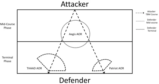
We present a networked TBM defense utilizing the Missile Defense Agency’s (MDA) defense-in-depth plan for a mid-course and terminal phase defense. For this scenario the defender seeks to protect two assets. This scenario places an Aegis air defense system at the mid-course point, a THAAD with the first defended asset, and a Patriot with the second defended asset. See Figure 1 for a detailed diagram of this scenario. All TBMs pass through the Aegis’ area of responsibility, and the Aegis has
an opportunity to fire up to two interceptors at each TBM. We allocate 12 intercep-tors to the Aegis, which constitutes half of the payload of the Aegis equipped ship [1]. The THAAD and the Patriot can only fire at TBMs targeting their defended asset, but they also have the opportunity to fire up to two interceptors at each TBM. The attacker fires a combination of traditional TBMs and multiple reentry vehicle (MeRV) TBMs. If the MeRV is missed (or not targeted) by the Aegis, it splits into three missiles (targets) before the THAAD or Patriot have an opportunity to fire at it. The TBMs, if missed or not fired at in the terminal phase, have a given probability of hitting its intended target. This probability of hit models the technical sophistication of the attacker’s weaponry (e.g., flight control, guidance, and warhead technology). If the TBM hits its targeted defended asset, it decrements the asset by a preassigned amount of one quarter of the asset’s total value. The defended asset can sustain up to four hits before being completely destroyed. A discount factor is used to model how many expected salvos the defender will encounter. See Davis et al. (2016) for a description of this modeling approach.
Attacker
Mid-Course Phase Terminal Phase Aegis AORTHAAD AOR Patriot AOR
Attacker TBM Course Defender Mid-course Defender Terminal
Defender
From this basic scenario, we develop 32 test instances by varying four of the problem features. We first varied the number of salvos the defender can expect to engage, or the duration of the attack, as indicated by γ. Exploratory simulations, based on the number of available interceptors in each phase, allowed us to choose two
γ-values, 0.8 and 0.9, to investigate the impact the expected number of salvos had on the ADP policy.
The second problem feature we varied was the enemy’s level of technological so-phistication – that is, the enemy may have fairly accurate TBMs or inaccurate TBMs. We chose a probability of hit of 0.8 for the technologically superior attacker and a probability of hit of 0.5 for the technologically inferior attacker.
The third problem feature we varied was the defender’s level of technological sophistication, seeking to capture the accuracy of the defender’s interceptors to suc-cessfully engage the TBMs. We chose a probability of kill for the technologically superior defender of 0.8, 0.9, and 0.85 for the Aegis, THAAD and Patriot, respec-tively. We chose a probability of kill for the technologically inferior defender of 0.7, 0.8, and 0.75, for the Aegis, THAAD, and Patriot respectively.
The fourth problem feature we varied was the defended asset value. We wanted to investigate how a higher, lower, or equal value of the defended assets protected by the THAAD and Patriot would affect the ADP policy. We assigned equal values of 24 for both Asset 1 and Asset 2 for the Low/Low case, values of 48 for Asset 1 and 24 for Asset 2 for the High/Low case, values of 24 for Asset 1 and 48 for Asset 2 in the Low/High case, and equal values of 48 for both Asset 1 and Asset 2 in the High/High case. Table 1 shows the problem feature settings for each test instance.
Table 1. Test Instances Problem Features Expected Conflict Duration Attacker’s Technological Sophistication Defender’s Technological Sophistication Defended Asset Values 1 Short (E[T] = 5) Low (pH = 0.5) Medium (pK = 0.7, 0.8, 0.75) Low/Low 2 Short (E[T] = 5) Low (pH = 0.5) Medium (pK = 0.7, 0.8, 0.75) High/Low 3 Short (E[T] = 5) Low (pH = 0.5) Medium (pK = 0.7, 0.8, 0.75) Low/High 4 Short (E[T] = 5) Low (pH = 0.5) Medium (pK = 0.7, 0.8, 0.75) High/High 5 Short (E[T] = 5) Low (pH = 0.5) High (pK = 0.8, 0.9, 0.85) Low/Low 6 Short (E[T] = 5) Low (pH = 0.5) High (pK = 0.8, 0.9, 0.85) High/Low 7 Short (E[T] = 5) Low (pH = 0.5) High (pK = 0.8, 0.9, 0.85) Low/High 8 Short (E[T] = 5) Low (pH = 0.5) High (pK = 0.8, 0.9, 0.85) High/High 9 Short (E[T] = 5) High (pH = 0.8) Medium (pK = 0.7, 0.8, 0.75) Low/Low 10 Short (E[T] = 5) High (pH = 0.8) Medium (pK = 0.7, 0.8, 0.75) High/Low 11 Short (E[T] = 5) High (pH = 0.8) Medium (pK = 0.7, 0.8, 0.75) Low/High 12 Short (E[T] = 5) High (pH = 0.8) Medium (pK = 0.7, 0.8, 0.75) High/High 13 Short (E[T] = 5) High (pH = 0.8) High (pK = 0.8, 0.9, 0.85) Low/Low 14 Short (E[T] = 5) High (pH = 0.8) High (pK = 0.8, 0.9, 0.85) High/Low 15 Short (E[T] = 5) High (pH = 0.8) High (pK = 0.8, 0.9, 0.85) Low/High 16 Short (E[T] = 5) High (pH = 0.8) High (pK = 0.8, 0.9, 0.85) High/High 17 Long (E[T] = 10) Low (pH = 0.5) Medium (pK =0.7, 0.8, 0.75) Low/Low 18 Long (E[T] = 10) Low (pH = 0.5) Medium (pK =0.7, 0.8, 0.75) High/Low 19 Long (E[T] = 10) Low (pH = 0.5) Medium (pK =0.7, 0.8, 0.75) Low/High 20 Long (E[T] = 10) Low (pH = 0.5) Medium (pK = 0.7, 0.8, 0.75) High/High 21 Long (E[T] = 10) Low (pH = 0.5) High (pK = 0.8, 0.9, 0.85) Low/Low 22 Long (E[T] = 10) Low (pH = 0.5) High (pK = 0.8, 0.9, 0.85) High/Low 23 Long (E[T] = 10) Low (pH = 0.5) High (pK = 0.8, 0.9, 0.85) Low/High 24 Long (E[T] = 10) Low (pH = 0.5) High (pK = 0.8, 0.9, 0.85) High/High 25 Long (E[T] = 10) High (pH = 0.8) Medium (pK = 0.7, 0.8, 0.75) Low/Low 26 Long (E[T] = 10) High (pH = 0.8) Medium (pK = 0.7, 0.8, 0.75) High/Low 27 Long (E[T] = 10) High (pH = 0.8) Medium (pK = 0.7, 0.8, 0.75) Low/High 28 Long (E[T] = 10) High (pH = 0.8) Medium (pK = 0.7, 0.8, 0.75) High/High 29 Long (E[T] = 10) High (pH = 0.8) High (pK = 0.8, 0.9, 0.85) Low/Low 30 Long (E[T] = 10) High (pH = 0.8) High (pK = 0.8, 0.9, 0.85) High/Low 31 Long (E[T] = 10) High (pH = 0.8) High (pK = 0.8, 0.9, 0.85) Low/High 32 Long (E[T] = 10) High (pH = 0.8) High (pK = 0.8, 0.9, 0.85) High/High
Experimental Design.
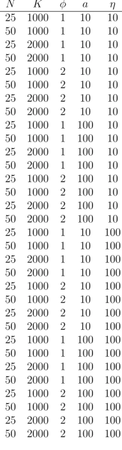
For each of the 32 test instances, we wish to determine the best parameter settings for Algorithms 1 and 2. We focus on parameters N, K, φ, a, and η. Table 2 shows the 2-level, 5-factor experimental design, and Table 3 shows the set of features for each design level of the φ factor. The levels for each factor were chosen based on initial experimental runs of the model. These experimental runs also suggested that the instrumental variables (IV) method for LSTD would not perform well for these instances, and so the IV method was not utilized.
Experimental Results.
For each test instance, we ran a full factorial experiment for three random number seeds (i.e., three replications) for a total of 96 runs. For each run, we recorded the mean and standard deviation, and calculated the difference between the ADP policy means and the means garnered from our two baseline policies. For each scenario, we chose the ADP policy (and noted the attendant parameter settings) that provided the largest difference between the baseline policies and the ADP policy.
Table 2. Experimental Design for Algorithmic Features N K φ a η 25 1000 1 10 10 50 1000 1 10 10 25 2000 1 10 10 50 2000 1 10 10 25 1000 2 10 10 50 1000 2 10 10 25 2000 2 10 10 50 2000 2 10 10 25 1000 1 100 10 50 1000 1 100 10 25 2000 1 100 10 50 2000 1 100 10 25 1000 2 100 10 50 1000 2 100 10 25 2000 2 100 10 50 2000 2 100 10 25 1000 1 10 100 50 1000 1 10 100 25 2000 1 10 100 50 2000 1 10 100 25 1000 2 10 100 50 1000 2 10 100 25 2000 2 10 100 50 2000 2 10 100 25 1000 1 100 100 50 1000 1 100 100 25 2000 1 100 100 50 2000 1 100 100 25 1000 2 100 100 50 1000 2 100 100 25 2000 2 100 100 50 2000 2 100 100
Table 3. Basis Function Features
φ φ0(S) φ1(S) φ2(S) φ3(S) φ4(S) φ5(S)
1 1 At Rxt Axt
2 1 Rx
4.2 Least Squares Policy Evaluation
Using the problem features and experimental design described in Section 4.1, we implemented the LSPE algorithm annotated in Algorithm 2. This required 3072 runs to perform the full factorial experiment for all problem and algorithmic features with three replications. The LSPE ADP algorithm provided a θ-vector for each of these 3072 runs. We then utilized a simulation to determine the mean performance and standard deviation for each of those 3072 θ-vectors. We executed 2000 simulation runs for eachθ-vector in order to gain confidence that we found an accurate mean.
We compared the ADP results to the two baseline policies. The first baseline policy (Baseline Policy 1) was to fire one interceptor at each incoming TBM (as long as the SAM site inventory allowed), and the second baseline policy (Baseline Policy 2)was to fire two interceptors at each TBM (if the SAM site inventory did not allow for firing two, only then would the SAM fire one). We executed 2000 simulation runs for the two baseline policies. In exploratory runs of the simulation, we found that firing one interceptor at each incoming TBM generally outperformed firing two interceptors for the problem features being explored. We compared the means of the policies found by our LSPE algorithms to the two baseline policies. The results for the best ADP policy versus the baseline polices for each scenario are shown in Table 4.
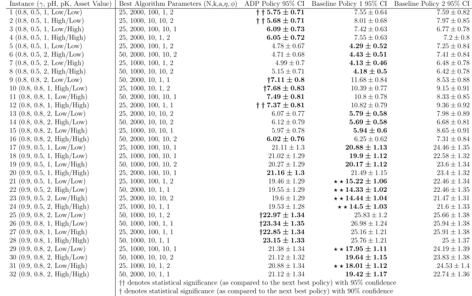
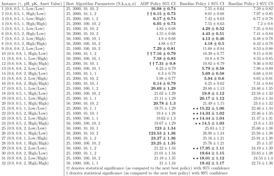
Table 4. LSPE Results - Quality of Solution Using Best θ-vector
Instance (γ, pH, pK, Asset Value) Best Algorithm Parameters (N,k,a,η, φ) ADP Policy 95% CI Baseline Policy 1 95% CI Baseline Policy 2 95% CI 1 (0.8, 0.5, 1, Low/Low) 25, 2000, 100, 1, 2 † †5.75±0.71 7.55±0.64 7.59±0.82 2 (0.8, 0.5, 1, High/Low) 25, 1000, 10, 10, 2 † †5.68±0.71 8.01±0.68 7.97±0.85 3 (0.8, 0.5, 1, Low/High) 25, 2000, 100, 10, 1 6.09±0.73 7.42±0.63 6.77±0.78 4 (0.8, 0.5, 1, High/High) 25, 2000, 10, 1, 2 6.05±0.72 7.55±0.63 7.2±0.8 5 (0.8, 0.5, 1, Low/Low) 25, 2000, 100, 1, 2 4.78±0.67 4.29±0.52 7.25±0.84 6 (0.8, 0.5, 2, High/Low) 50, 2000, 100, 10, 2 4.71±0.68 4.43±0.51 7.41±0.84 7 (0.8, 0.5, 2, Low/High) 25, 1000, 100, 1, 2 4.99±0.7 4.13±0.46 6.48±0.78 8 (0.8, 0.5, 2, High/High) 50, 1000, 10, 10, 2 5.15±0.71 4.18±0.5 6.42±0.78 9 (0.8, 0.8, 2, Low/Low) 50, 2000, 10, 1, 1 †7.11±0.8 11.68±0.84 8.53±0.88 10 (0.8, 0.8, 1, High/Low) 25, 1000, 10, 1, 2 †7.68±0.83 10.39±0.77 9.15±0.91 11 (0.8, 0.8, 1, Low/High) 50, 2000, 100, 10, 1 7.49±0.81 10.8±0.78 8.33±0.85 12 (0.8, 0.8, 1, High/High) 25, 2000, 100, 1, 1 † †7.37±0.81 10.82±0.79 9.36±0.92 13 (0.8, 0.8, 2, Low/Low) 25, 2000, 10, 10, 2 6.07±0.77 5.79±0.58 7.98±0.89 14 (0.8, 0.8, 2, High/Low) 50, 2000, 10, 10, 2 6.12±0.79 5.69±0.58 6.68±0.81 15 (0.8, 0.8, 2, Low/High) 25, 1000, 10, 10, 1 5.97±0.78 5.94±0.6 8.65±0.91 16 (0.8, 0.8, 2, High/High) 50, 2000, 100, 10, 2 6.02±0.76 6.25±0.62 7.31±0.84 17 (0.9, 0.5, 1, Low/Low) 25, 1000, 100, 10, 1 21.11±1.3 20.88±1.13 24.46±1.35 18 (0.9, 0.5, 1, High/Low) 25, 1000, 100, 10, 1 21.02±1.29 19.9±1.12 22.58±1.32 19 (0.9, 0.5, 1, Low/High) 50, 1000, 100, 10, 2 20.27±1.29 20.17±1.12 23.6±1.34 20 (0.9, 0.5, 1, High/High) 25, 2000, 100, 10, 1 21.16±1.3 21.49±1.15 23.4±1.32 21 (0.9, 0.5, 1, Low/Low) 25, 1000, 100, 1, 2 19.46±1.29 ? ?15.22±1.06 22.46±1.34 22 (0.9, 0.5, 2, High/Low) 50, 2000, 10, 1, 1 19.55±1.29 ? ?14.33±1.02 22.46±1.35 23 (0.9, 0.5, 2, Low/High) 25, 2000, 10, 10, 2 19.6±1.29 ? ?14.44±1.04 21.47±1.31 24 (0.9, 0.5, 2, High/High) 25, 1000, 10, 1, 1 19.53±1.28 ? ?14.5±1.03 21.6±1.33 25 (0.9, 0.8, 2, Low/Low) 50, 1000, 10, 1, 2 †22.97±1.34 25.83±1.2 25.66±1.38 26 (0.9, 0.8, 1, High/Low) 50, 1000, 100, 1, 1 †23.34±1.35 26.98±1.24 25.94±1.38 27 (0.9, 0.8, 1, Low/High) 25, 2000, 100, 1, 1 †22.85±1.34 25.16±1.21 25.91±1.38 28 (0.9, 0.8, 1, High/High) 50, 1000, 10, 1, 1 23.15±1.33 25.76±1.21 25±1.37 29 (0.9, 0.8, 2, Low/Low) 25, 1000, 100, 10, 1 21.38±1.34 ? ?17.95±1.11 24.19±1.39 30 (0.9, 0.8, 2, High/Low) 50, 1000, 10, 10, 2 21.12±1.32 19.64±1.15 23.83±1.38 31 (0.9, 0.8, 2, Low/High) 25, 1000, 10, 1, 2 20.88±1.34 ? ?18.01±1.12 24.53±1.4 32 (0.9, 0.8, 2, High/High) 50, 2000, 10, 1, 1 21.12±1.34 19.42±1.17 22.74±1.36
††denotes statistical significance (as compared to the next best policy) with 95% confidence
†denotes statistical significance (as compared to the next best policy) with 90% confidence
The LSPE policy achieves statistically significant improvement over the two base-line policies in 8 of the 32 test instances. The instances that show LSPE policy superiority at the 95% confidence level are 1, 2, and 12. Instances 9, 10, 25, 26, and 27 show statistical significance at the 90% confidence level. LSPE attains the best mean result in 14 of the 32 instances. We see that LSPE outperforms the baseline policies when the duration of the conflict is short or when the enemy has weapons with a high probability of hit. It is not surprising that in circumstances where if missed the incoming TBM has a high likelihood of damaging its targeted asset that the LSPE policy outperforms the baseline policies, but it is interesting that in shorter duration conflicts when the two baseline policies show very similar means that the ADP is able to outperform at a statistically significant level.
Baseline Policy 1 outperforms LSPE in Instances 21, 22, 23, 24, 29, and 31 at the 95% confidence level. Examining these instances, we find common characteristics: long duration conflict where the attacker had lower quality weapons and the defender had higher quality weapons.
It is of further interest that Baseline Policy 2, which is currently the Army’s implemented policy, is never significantly better than the LSPE policy or Baseline Policy 1. This suggests that as the military moves to an integrated, defense-in-depth strategy it needs to consider a different firing policy for networked air defense systems with both mid-course and terminal systems.
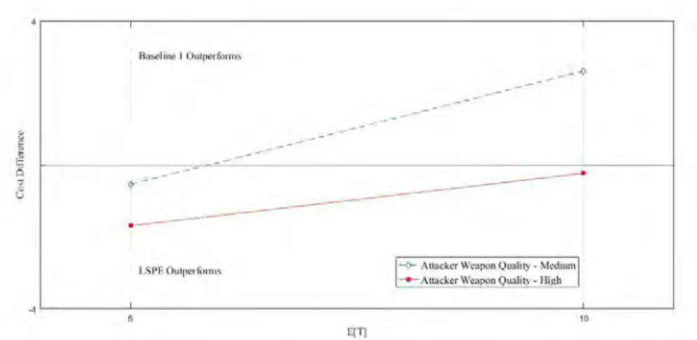
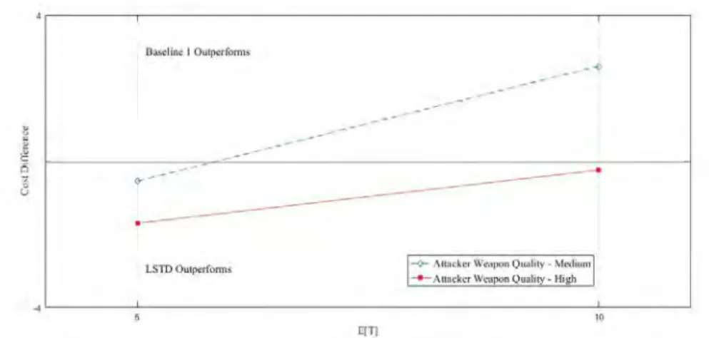
Figure 2. Cost Difference between High and Low Attacker Weapon Quality
Figure 2 highlights the cost difference between LSPE and Baseline Policy 1 when we look at the two different levels of attacker weapon quality for short and long duration conflicts. In this we observe that for high quality attacker weapons LSPE performs better than the baseline policy regardless of conflict duration, but for low quality attacker weapons Baseline Policy 1 is superior for long duration conflicts. Note that this graphic implies a linear relationship that might not exist.
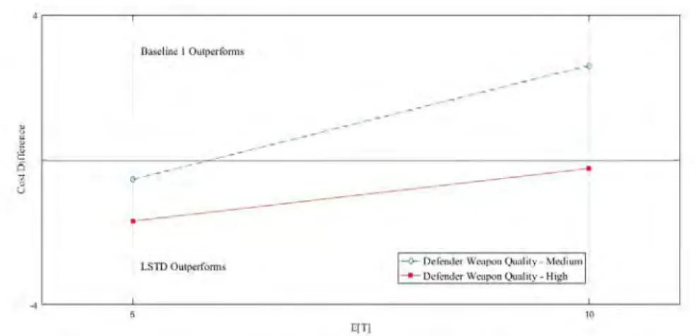
Figure 3. Cost Difference between High and Medium Defender Weapon Quality
Figure 3 highlights the cost difference between LSPE and Baseline Policy 1 when we look at the two different levels of defender weapon quality for short and long
LSPE performs better than the baseline policy regardless of conflict duration, but for high quality defender weapons Baseline Policy 1 is always superior. Note that this graphic implies a linear relationship that might not exist.
Table 5. LSPE Results - Robustness
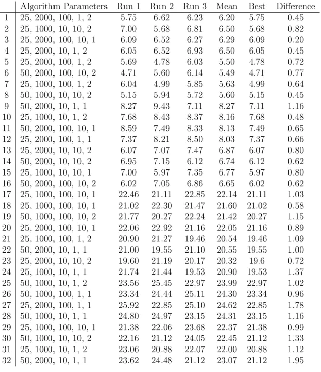
Algorithm Parameters Run 1 Run 2 Run 3 Mean Best Difference
1 25, 2000, 100, 1, 2 5.75 6.62 6.23 6.20 5.75 0.45 2 25, 1000, 10, 10, 2 7.00 5.68 6.81 6.50 5.68 0.82 3 25, 2000, 100, 10, 1 6.09 6.52 6.27 6.29 6.09 0.20 4 25, 2000, 10, 1, 2 6.05 6.52 6.93 6.50 6.05 0.45 5 25, 2000, 100, 1, 2 5.69 4.78 6.03 5.50 4.78 0.72 6 50, 2000, 100, 10, 2 4.71 5.60 6.14 5.49 4.71 0.77 7 25, 1000, 100, 1, 2 6.04 4.99 5.85 5.63 4.99 0.64 8 50, 1000, 10, 10, 2 5.15 5.94 5.72 5.60 5.15 0.45 9 50, 2000, 10, 1, 1 8.27 9.43 7.11 8.27 7.11 1.16 10 25, 1000, 10, 1, 2 7.68 8.43 8.37 8.16 7.68 0.48 11 50, 2000, 100, 10, 1 8.59 7.49 8.33 8.13 7.49 0.65 12 25, 2000, 100, 1, 1 7.37 8.21 8.50 8.03 7.37 0.66 13 25, 2000, 10, 10, 2 6.07 7.07 7.47 6.87 6.07 0.80 14 50, 2000, 10, 10, 2 6.95 7.15 6.12 6.74 6.12 0.62 15 25, 1000, 10, 10, 1 7.00 5.97 7.35 6.77 5.97 0.80 16 50, 2000, 100, 10, 2 6.02 7.05 6.86 6.65 6.02 0.62 17 25, 1000, 100, 10, 1 22.46 21.11 22.85 22.14 21.11 1.03 18 25, 1000, 100, 10, 1 21.02 22.30 21.47 21.60 21.02 0.58 19 50, 1000, 100, 10, 2 21.77 20.27 22.24 21.42 20.27 1.15 20 25, 2000, 100, 10, 1 22.06 22.92 21.16 22.05 21.16 0.89 21 25, 1000, 100, 1, 2 20.90 21.27 19.46 20.54 19.46 1.09 22 50, 2000, 10, 1, 1 21.00 19.55 21.10 20.55 19.55 1.00 23 25, 2000, 10, 10, 2 19.60 21.19 20.17 20.32 19.6 0.72 24 25, 1000, 10, 1, 1 21.74 21.44 19.53 20.90 19.53 1.37 25 50, 1000, 10, 1, 2 23.56 25.45 22.97 23.99 22.97 1.02 26 50, 1000, 100, 1, 1 23.34 24.44 25.11 24.30 23.34 0.96 27 25, 2000, 100, 1, 1 25.92 22.85 25.10 24.62 22.85 1.78 28 50, 1000, 10, 1, 1 24.80 24.97 23.15 24.31 23.15 1.16 29 25, 1000, 100, 10, 1 21.38 22.06 23.68 22.37 21.38 0.99 30 50, 1000, 10, 10, 2 22.16 21.12 24.05 22.45 21.12 1.33 31 25, 1000, 10, 1, 2 23.06 20.88 22.07 22.00 20.88 1.12 32 50, 2000, 10, 1, 1 23.62 24.48 21.12 23.07 21.12 1.95
Table 5 shows the LSPE-determined three-run averages for the θ-vectors for each replication of the 32 instances. These three-run averages show a general robustness
across the θ-vectors garnered from the given parameter settings. For most of the instances, we have a less than 1 point difference between the best mean and the aver-age mean. Though this would impact the statistical significance of those parameter settings versus the baseline policies, it does not indicate that any of the chosen best
θ-vectors were simply outliers. This result suggests an overall robustness with respect to the consistency of performance of the LSPE algorithm.
Meta Analysis
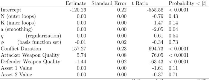
Table 6. Parameter Estimates - LSPE
Estimate Standard Error t Ratio Probability <|t|
Intercept -120.26 0.22 -555.56 <0.0001
N (outer loops) 0.00 0.00 -0.79 0.43
K (inner loops) 0.00 0.00 1.47 0.14
a (smoothing) 0.00 0.00 -2.05 0.04
η (regularization) 0.00 0.00 0.61 0.54
φ (basis function set) -0.01 0.02 -0.34 0.73
Conflict Duration 157.27 0.23 694.73 <0.0001
Attacker Weapon Quality 5.74 0.08 76.05 <0.0001
Defender Weapon Quality -1.44 0.02 -63.43 <0.0001
Asset 1 Value 0.00 0.00 -1.61 0.11
Asset 2 Value 0.00 0.00 -0.37 0.71
R-Square Adj 0.99
When examining the parameter estimates in Table 6, we see that conflict duration, attacker weapon quality, and defender weapon quality have the largest impact on the change in the mean of the damage caused by the incoming TBMs. Although not statistically significant at a 95% confidence level, the Asset 1 value factor appears to explain more of the variation than the N, η, φand the Asset 2 value factors. Recall that Asset 1 is protected by the THAAD air defense system and the THAAD had the highest pK across all scenarios. This suggests that having the more effective air defense system co-located with the higher value asset could lead to more impact in
Examining the parameter settings for the ADP algorithm, we observe that the smoothing component explains a significant portion of the variation (with a 0.04 p-value). Although the number of inner loops (K) is not statistically significant, it does explain more variation than the other parameter settings. It is likely that the number of outer loops (N) did not have more impact on the mean because the smoothing coefficient did have an impact, and new information garnered from a higher number of outer loops received very little weight. We likely did not have a large enough difference in the number of inner loops, and had we had time to perform 4000 inner loops, we might have seen this coefficient become statistically significant. Since the
φ did not have an impact we might benefit from searching for other sets of basis functions that perform better than the baseline policies.
4.3 Least Squares Temporal Difference
Using the problem features and experimental design described in Section 4.1 we implemented the LSTD algorithm annotated in Algorithm 1. This required 3072 runs to perform the full factorial experiment of all problem and algorithmic features with three replications. The LSTD ADP algorithm provided a θ-vector for each of these 3072 runs. We then utilized a simulation to determine the performance in terms of the mean and standard deviation for each of those 3072θ-vectors. We executed 2000 simulation runs to ensure we had confidence in our garnered mean.
We compared these means to the means for the two baseline policies. We compared the means of our LSTD algorithms to the two baseline policies. These results for the best θ-vector versus the baseline for each scenario is shown on Table 7.
![Table 1. Test Instances Problem Features Expected Conflict Duration Attacker’s TechnologicalSophistication Defender’s TechnologicalSophistication Defended AssetValues 1 Short (E[T ] = 5) Low (pH = 0.5) Medium (pK = 0.7, 0.8, 0.75) Low/Low 2 Short (E[T ] =](https://thumb-us.123doks.com/thumbv2/123dok_us/10217763.2925624/40.918.141.796.296.951/instances-features-expected-conflict-duration-technologicalsophistication-technologicalsophistication-assetvalues.webp)