NBER WORKING PAPER SERIES
THE EFFECT OF SCHOOLING AND ABILITY ON ACHIEVEMENT TEST SCORES
Karsten Hansen James J. Heckman Kathleen J. Mullen Working Paper 9881
http://www.nber.org/papers/w9881
NATIONAL BUREAU OF ECONOMIC RESEARCH 1050 Massachusetts Avenue
Cambridge, MA 02138 July 2003
This research is supported by grants from NICHD-40-4043-000-85-261 and NSF SES-0099195.We thank Chris Winship for a stimulating discussion which influenced this paper. (See his related research reported in Winship, 2001). We have benefitted from numerous comments by Derek Neal and Chris Winship on various aspects of this paper. We also thank Joseph Kaboski, Salvador Navarro, Sergio Urzua, participants of the Empirical Economics workshop and the Theory and Econometrics workshop at the University of Chicago, and an anonymous referee for helpful comments. The views expressed herein are those of the authors and not necessarily those of the National Bureau of Economic Research.
©2003 by Karsten Hansen, James J. Heckman, and Kathleen J. Mullen. All rights reserved. Short sections of text, not to exceed two paragraphs, may be quoted without explicit permission provided that full credit, including © notice, is given to the source.
The Effect of Schooling and Ability on Achievement Test Scores Karsten Hansen, James J. Heckman, and Kathleen J. Mullen NBER Working Paper No. 9881
July 2003
JEL No. C35, C15, I21
ABSTRACT
This paper develops two methods for estimating the effect of schooling on achievement test scores that control for the endogeneity of schooling by postulating that both schooling and test scores are generated by a common unobserved latent ability. These methods are applied to data on schooling and test scores. Estimates from the two methods are in close agreement. We find that the effects of schooling on test scores are roughly linear across schooling levels. The effects of schooling on measured test scores are slightly larger for lower latent ability levels. We find that schooling increases the AFQT score on average between 2 and 4 percentage points, roughly twice as large as the effect claimed by Herrnstein and Murray (1994) but in agreement with estimates produced by Neal and Johnson (1996) andWinship and Korenman (1997). We extend the previous literature by estimating the impact of schooling on measured test scores at various quantiles of the latent ability distribution.
Karsten Hansen James J. Heckman
Kellogg School of Management Department of Economics Northwestern University The University of Chicago
Evanston, IL 60657 1126 East 59th Street
[email protected] Chicago, IL 60637 and NBER
[email protected] Kathleen J. Mullen
Department of Economics The University of Chicago 1126 East 59th Street Chicago, IL 60637
1
Introduction
There are two widely held and mutually inconsistent conceptions of ability and scholastic achievement tests. The first view claims that cognitive ability is essentially fixed at a relatively early age (around age seven) and is virtually unchanged afterward. According to this view, achievement tests and IQ tests measure the same fundamental cognitive skill. The correlation between IQ and achievement tests is high and proponents of this view use these two types of tests interchangeably. According to scholars who advocate this point of view, schooling and other influences barely budge measured IQ. (See the evidence summarized in Herrnstein and Murray, 1994, Appendix 2.) A consensus estimate in this literature is that a year of schooling raises measured IQ by about one point (Jencks, 1972; Herrnstein and Murray, 1994).1 A second widely held view claims that schooling raises achievement measured by tests and more successful types of schooling raise measured achievement more. This is the premise of large scale testing programs designed to monitor the performance of schools. Debates about the effectiveness of vouchers and interventions hinge on their effects on measured achievement (see, e.g., Hanushek, 2002). This literature implicitly separates out latent ability (IQ) from measured ability and views schooling as a mechanism for either enhancing or revealing ability. Proponents of this view argue that schooling can increase measured ability by as much as 2 to 4 points (Winship and Korenman, 1997; Neal and Johnson, 1996), or 2.9 to 5.7 AFQT points (2.7 to 5.4 percentage points).
This paper presents evidence that the measure of IQ used by Herrnstein and Murray is strongly affected by schooling. Postulating that latent ability cannot be affected by schooling, we test whether manifest ability is affected by schooling when both schooling and manifest ability are affected by latent ability. Manifest ability is widely regarded as a determinant of socioeconomic success. Gaps in test scores across socioeconomic groups are widely viewed as a major source of social problems (Jencks and Phillips, 1998; Herrnstein and Murray, 1994). We examine whether measured ability gaps can be eliminated by schooling. Our measures of ability are the ASVAB achievement (competency) tests used to screen persons entering the military. ASVAB stands for Armed Services Vocational Aptitude Battery and is described in more detail below. We find that schooling, especially in the high school years, is an important determinant of measured achievement. It operates differently at different latent ability levels.
In order to establish these conclusions, we need to address the problem of reverse causality. There is a well-established empirical regularity that measured test scores predict schooling. Individuals choose to attend school in part based on their own intelligence which is measured by test scores. In addition, admission into colleges and fellowship support is based, in part, on scores on tests like the Scholastic Assessment Test (SAT). The central econometric question addressed in this paper is how to characterize and solve the problem of joint causality: schooling causing test scores and test scores causing schooling.
1IQ is assumed to have mean 100 and standard deviation 15. Many of the papers in the literature obtain estimates
using the Armed Forces Qualification Test (AFQT), the test used in this paper, which has a scale of 0-105. Typically estimates are converted into “IQ points” by computing the effect of education in terms of standardized AFQT score and then, assuming that a standard deviation increase in AFQT is equivalent to a standard deviation increase in IQ score, by further multiplying by 15. Herrnstein and Murray (1994) estimate an increase of 1.1 IQ points per year of education, or 1.6 AFQT points (1.5 percentage points), using our estimate of the standard deviation of AFQT, 21.6.
Our solution is based on a model of test scores as manifestations of latent ability (and other determinants) with schooling determined by latent ability (and other determinants). Our framework accounts for ceiling effects (on some easy tests, students with very different ability levels get perfect scores) and endogeneity of schooling (which includes choice of date of entry into schooling as well as choice offinal schooling level). Wefind that the effects of schooling on test scores for a given level of ability are approximately linear across schooling levels. Effects are slightly larger for those with lower ability. Schooling increases the AFQT score on average between 2 and 4 percentage points. This is roughly twice as large as the effect claimed by Herrnstein and Murray (1994).
The plan of this paper is as follows. Section 2 presents our framework and discusses some important conceptual issues. Section 3 applies the method of control functions, developed by Heckman (1976, 1980) and Heckman and Robb (1985, 1986), to identify schooling effects on tests using a special feature of the National Longitudinal Survey of Youth (NLSY) data. A nonparametric version of the method is developed, but it suffers from certain practical limitations in more general cases. Section 4 presents a parametric econometric model motivated by choice theory for the joint determination of schooling and test scores. This method allows us to supplement the nonparametric control function method to impose additional identifying information to develop a method for determining the effects of schooling on test scores in more general data sets than the NLSY and to account for ceiling effects on tests. Section 5 presents empirical results. Section 6 concludes. Appendix A describes the data. The estimation algorithm for the control function approach is presented in Appendix B. The likelihood and the Bayesian computational methods used to estimate it are presented in Appendix C.
2
The Relationship Between Ability and Schooling
LetT(s)be the test score of a person withsyears of schooling at the time the test is taken. For notational simplicity, we keep implicit the conditioning on all other variables that determineT(s)except latent ability f. The other variables might include age, socioeconomic status of the parents, and other environmental and genetic factors. We account for some of these additional variables in our empirical work.
Our model of test scores is based on an extension of the factor analysis model used in psychometrics (see e.g., Lord and Novick, 1968). Test score T(s) is a manifestation of latent ability f mediated by schooling:
T(s) =µ(s) +λ(s)f +ε(s) (1)
where it is assumed thatε(s)is independent off. Bothf andε(s) are assumed to have zero means. This amounts to a normalization and a definition of the mean, µ(s). We extend the standard model of factor analysis by allowing the level ofsselected to depend onf. For externally-manipulated levels of schooling, µ(s) in equation (1) is the effect of schooling that is uniform across latent ability levels and λ(s) is the effect of schooling on revealing or transforming latent ability f. The marginal causal effects of changing schooling froms0 to s on levels and slopes are µ(s)−µ(s0) andλ(s)−λ(s0) respectively using the usual ceteris paribus logic familiar to all economists.2
The psychometric and educational testing literatures are fundamentally ambiguous about what con-stitutes cognitive ability. Is it f, T(s), µ(s) or µ(s) +λ(s)f? Neal and Johnson (1996), Winship and Korenman (1997), Winship (2001), and Herrnstein and Murray (1994) take measured test scores (T(s)) to be cognitive ability. Yet the logic of IQ testing interprets f as cognitive ability. A reinterpretation of equation (1) writes λ(s)f as ability determined at schooling level s. Knowing only T(s) and S = s, we cannot decide which of these interpretations is correct. Without further information, the model is funda-mentally underidentified because we do not observe f. We can identify the combination of parameters in
E(T(s)|S =s) =µ(s) +λ(s)E(f|S=s) +E(ε(s)|S =s) (2) but the causal status of an estimated effect ofS is unclear because bothE(f |S=s)andE(ε(s)|S =s) may depend on S. Thus latent cognitive ability(f)may determine S and so may measured ability (T(s) and hence ε(s) given f). If the test studied does not directly affect schooling decisions, e.g. through its use in admission criteria, as is the case for the test analyzed in this paper, then E(ε(s)|S=s) = 0.3
The empirical literature recognizes the problem of reverse causality, and adopts different strategies for identifying different parameters. Herrnstein and Murray (1994) and Winship and Korenman (1997) implicitly adopt µ(s) as their parameter of interest, assume thatµ(s) =sβ (linearity) and use an “early” test score (obtained at an earlier age) to proxyf.4 Let proxy P be
P =γ0+γ1f +ε(P) (3)
wheref andε(P)are independent, andγ0,γ1 are assumed not to be functions of theS in (1). Solving for f and substituting into (1) we obtain
T(s) =µ(s)−λ(s)γ0 γ1 +λ(s) γ1 P + · ε(s)− λ(s)ε(P) γ1 ¸ . (4)
Observe that the composite error is correlated with P unless P is a perfect proxy for f (ε(P) = 0), the implicit assumption used by Herrnstein and Murray (1994).5 Herrnstein and Murray also implicitly
assume that λ(s) does not depend ons. Then, using ordinary least squares applied to (4), they estimate the marginal effect of schooling which in their setup is β (µ(s) =sβ). If λ(s) =λ, butε(P) 6= 0, and if λγ1 >0(so thatf affectsP andT(s)in the same way), then least squares based on (3) is upward biased. More generally, ifλdepends ons, the bias is ambiguous and depends on specific parameter configurations. The combination of parameters µ(s)−λ(s)γ0
γ1 becomes the implicit parameter estimated and it does not
answer the questions posed in the literature.
Winship and Korenman (1997) consider the problem of measurement error in their proxyP. They draw on work by Ashenfelter and Krueger (1994) who claim that the reliability (the proportion of variance of P that is true, γ2
1σ2f, relative to the total variance γ21σ2f +σ2ε) of IQ measures is typically above 0.9.
nonseparable model would be desirable but is beyond the scope of this paper.
3Even though the tested know their scores they are not directly used by schools orfirms to screen persons and we assume
that they do not affect subsequent actions.
4These authors also include additional control variables which we do not discuss. 5Pakes and Olley (1995) make the same assumption in a different context.
Winship and Korenman carry out a variety of sensitivity analyses, estimating the model under different assumptions about the reliability of the early IQ score, which they let take on values between 0.8 and1. They obtain a wide range of estimates of the effect of schooling on AFQT, from1.5to5points. Correcting for measurement error under what Winship and Korenman believe to be “reasonable assumptions about the extent of measurement error,” they estimate the effect of education to be 2.7 IQ points per year of school and they state that “a year of education most likely increases IQ by somewhere between 2 and 4 points.”
Neal and Johnson take a different approach. They choose β in the specification µ(s) = sβ as their parameter of interest and use month of birth (which determines years of schooling attained by a given birth cohort) as an instrument to avoid dependence ofSonf.6 This forced variation in schooling attained
among children of the same nominal birth cohort is a source of identifying variation. We estimate a richer set of parameters and consider how schooling affects test scores at different levels of the latent ability distribution. However, our estimates of the same parameter are in agreement with theirs.
A variety of other studies, surveyed by Ceci (1991), rely on various “natural experiments” of uncertain quality. Winship and Korenman (1997) survey and criticize this literature.
In this paper, we estimate µ(s) and λ(s) for different levels of schooling without imposing the para-metric restrictions used in the previous literature. We explicitly account for the endogeneity of completed schooling. In addition we estimate the distribution of latent ability (f) and compare it with measured ability. We can identify the effect of schooling on measured test scores at different latent ability(f)levels. This allows us to identify where in the overall distribution of ability schooling interventions are the most effective. We first develop estimators based on the principle of control functions.
3
Simple Identi
fi
cation Strategies Based on Control Functions
Our first approach to this problem exploits an unusual feature of the NLSY data. The test we study is given to a nationally representative sample of people. Some people who take the test are in school while others have finished school. We observe completed schooling for all individuals. Let ST denote schooling
that a person has at the date of the test. We observe the test scoreT(ST)which can be expressed as
T(ST) =µ(ST) +λ(ST)f +ε(ST). (5)
LettingS denote thefinal level of schooling that is actually attained,S ≥ST. Let Abe the age at which
a person is tested. If we redefine age so that schooling starts at age 0 and if we assume that dropouts do not return to school, then we observe ST = A < S if the test date comes before a person has completed
his schooling.7 If he has completed schooling by the time of the test, then we observeS T =S.
Using the control function approach introduced in Heckman (1976, 1980) and Heckman and Robb (1985, 1986), and assuming no maturation effects (no independent effect of age on performance on the
6In most school districts, in a given year any 5 year-old child whose birthday falls after October 1 must wait to start
school in the following year.
test) and that everyone starts school at the same age, we may write observed tests conditional on final schooling and schooling at the test date as
E(T(ST)|ST =sT, S =s) = µ(sT) +λ(sT)E(f|ST =sT, S =s) (6)
+E(ε(ST)|ST =sT, S =s).
To simplify the notation we keep other conditioning variables implicit.
Because sampling is random across ages, if individuals consider only their final schooling level when making schooling decisions, irrespective of their path to schooling and there is no dropping out and re-entry, conditional on S =s the observed ST is random with respect to f. Thus E(f |ST =sT, S =s) =
E(f | S = s). Further, if the test is not used to make decisions about schooling, E(ε(ST) | ST = sT,
S =s) = 0.
Under these assumptions we obtain
E(T(ST)|ST =sT, S =s) =µ(sT) +λ(sT)E(f |S=s). (7)
From this equation it is clear that we cannot identify the scale off without some normalization. Setting λ(1) = 1 is one such normalization. We can identify λ(sT) up to the normalization because for two
different schooling levelss, s0 ≥s
T, s6=s0,
E(T(ST)|ST =sT, S=s)−E(T(ST)|ST =sT, S =s0) =λ(sT)[E(f |S =s)−E(f |S =s0)].
Assuming λ(sT)6= 0, we may form the ratio
E(T(ST)|ST =s0T, S =s)−E(T(ST)|ST =s0T, S =s0) E(T(ST)|ST =sT, S =s)−E(T(ST)|ST =sT, S =s0) = λ(s 0 T) λ(sT)
for two valuessT 6=s0T, both less than or equal to s, s0. Therefore with one normalization we can identify
all of the λ(sT), sT = 1, ...,S¯−1 (we cannot identifyλ
¡¯
S¢ because there is only one possible value of s for ST = ¯S).
Taking expectations with respect to ST alone we obtain
E(T(ST)|ST =sT) =µ(sT) +λ(sT)E[f|ST =sT].8 (8)
Recall that we knowλ(sT), sT = 1, . . . ,S¯−1,from the preceding argument. Subtracting (8) from (7) we
obtain
E(T(ST)|ST =sT, S=s)−E(T(ST)|ST =sT) =λ(sT)[E(f |S =s)−E(f |ST =sT)]
so we can identify fors ≥sT, sT = 1, . . . ,S¯−1,
E(f |S =s)−E(f |ST =sT) =
E(T(ST)|ST =sT, S =s)−E(T(ST)|ST =sT)
λ(sT)
. (9)
Let E(f | S = s) = as and E(f |ST =sT) = bsT. We can form a matrix of the following identifiable
combination of parameters:
8Note thatE(ε(S
aS¯−b1 aS¯−1−b1 ... ... ... a1−b1 aS¯−b2 aS¯−1−b2 ... ... ... ∼ ... ... ... ... ∼ ∼ aS¯−b¯S−1 aS¯−1−b¯S−1 ... ∼ ∼ ∼ ∼ ∼ ... ∼ ∼ ∼
where “∼” in a cell denotes the absence of data on the entry. We also know as a consequence ofE(f) = 0 that if we define Pj = Pr(S =j) ¯ S X j=1 ajPj = 0. (10)
Letting Pej be Pr(ST =j), we also obtain
¯
S
X
j=1
bjPej = 0. (11)
Taking a weighted sum across row 1 of the matrix, we identifyb1 since ¯ S X j=1 Pj(aj −b1) = ¯ S X j=1 ajPj −b1 ¯ S X j=1 Pj =−b1
by (10) and the fact that PSj¯=1Pj = 1. Going across the first row element by element, we obtain aj, j =
1, . . . ,S. Going down the¯ first column, we obtain the remainingbj, j = 1, . . . ,S¯−1. Using (11) we identify
bS¯.Thus the model is fully identified except forλ¡S¯¢.
Attractive as these results are, there are three reasons to be cautious about estimates derived from this identification strategy: (a) Age effects (maturation effects) may affect test scores independently of any effect of schooling because persons may acquire life experiences that raise their test scores independently of their schooling at the date of the test. Our procedure has to be modified to distinguish age effects from schooling effects. (b) Persons start school at different ages. Less able people (those with lower f) may start school at later ages, making an assumption of an identical school starting age for all persons problematic. Simply conditioning on the starting age N to solve this problem is not satisfactory given its likely dependence on f. (c) In principle there might be a separate N effect on test scores apart from the dependence of N on f if there are discouragement effects (students older than their classmates may feel inferior and be less motivated). The confluence of an endogenous N and independent age effects is problematic.
Modeling the starting age N along with the schooling level S does not pose any conceptually new problem as long as there are no age at test effects. We can use different(ST, N),(S, N)pairs and replace
(ST, S) in the preceding analysis. Data cells may thin out but the previous identification strategy works.
Allowing for age in addition to N produces a fundamental identification problem if we maintain the “no return to school for dropouts” assumption. Observe that by definitionST = min{A−N, S}, so that
S, ST and A−N cannot be freely varied. A more general model that incorporates age and entry writes
date of the test, S is the final level of schooling attained and N is the age at which the person enters school. For simplicity normalizeN = 0 to be the “normal age” of starting school. IfA andST both affect
the measured test score directly, while S and N do not directly affect the test score but potentially are stochastically dependent on latent ability f, we may write
T(A, ST, S, N) =µ(A, ST) +λ(A, ST)f +ε(A, ST).9 (12)
Then conditioning on observable (A, ST, S, N) we obtain
E(T(A, ST, S, N)|A=a, ST =sT, S =s, N =n) =µ(a, sT) +λ(a, sT)E(f|S =s, N =n) (13)
where we assumeε(A, ST)is independent of all other variables. Observe that whenST < S, fixingN and
ST determinesA:
A=ST +N (14)
This exact linear dependence does not apply to persons with completed schooling (ST = S). In that
subpopulation, S and ST cannot be independently varied so the control function identification strategy
previously developed breaks down but the exact linear dependence (14) does not hold so that we can independently varyA andST =S for eachN. If we parameterizeµ(A, ST)andλ(A, ST), we can identify
separate effects of age and schooling at the test date.10 With sufficient structure, we can extrapolate µ(A, ST) and λ(A, ST) back to ages and schooling levels at schooling levels ST < S. This method is
pursued in Section 4.
In our data, there are effectively two starting ages N ∈ N ={0,1}. Given our “no return to school for dropouts” assumption, in the sample S > ST, people who start school one year later are also one
year older at schooling level ST than are people who start school at a normal age. We cannot identify a
separateN effect from anA effect.
If we condition on each value of N =nand repeat the preceding identification argument for each N, we identify µ(sT, n) and λ(sT, n), s, s0 ≥ sT from the sample S ≥ ST by conditioning on ST = sT and
N = n in (8). When N = 0, ST = A if schooling is incomplete at the test date (S > ST). We identify
a joint schooling and age effect for each N. When N = 1, we can identify the effect of being one year older onµ(sT) andλ(sT) for samples in whichS > ST. This effect is indistinguishable from the effect of
starting one year later. We can test for an age (at test or entry) effect by testingµ(sT,0) =µ(sT,1)and
λ(sT,0) =λ(sT,1).11 This argument can be modified in a straightforward way to account for the case of
more than two elements inN.
While intuitively appealing, the method based on control functions does not exploit all of the infor-mation in the S = ST sample. Data where S = ST is the more commonly occurring case. It is not
9IfNcausally affects the test, then (12) is modified to readT(A, S
T, S, N) =µ(A, ST, N)+λ(A, ST, N)f+ε(A, ST, N). 10Thus withµ(A, S
T) =ϕ1(A) +ϕ2(ST)andλ(A, ST) =η1(A) +η2(ST)we can break these linear dependencies.
Multi-plicative versions can work as well. This is the strategy used in section 4 to achieve identification of these effects. See the closely related identification analysis of Heckman and Vytlacil (2001).
11Observe that for persons for whomS =S
T, age at test is not restricted by (14). Thus we can in principle identify age
effects when we useS =ST observations, but we cannot use the control function method developed in this section to solve
straightforward to use the control function method to account for ceiling effects. When S = ST, it is
possible in principle to isolate separate A, N andS effects. We now present a different method designed to analyze the entire sample more fully.
4
A Discrete-Continuous Econometric Model of Schooling and
Test Scores
This section develops a more explicitly structured semiparametric model that does not rely on special features of the NLSY data and that enables us to condition morefinely. The model also enables us to link our work to more conventional models of schooling and wages, and identify separateS, A andN effects. Initially we assume S =ST and then we extend the analysis to allow for the caseS > ST.
Unlike the control function method developed in Section 3, the method discussed in this section requires more than one test. Suppose that we have data on K (≥2) tests associated with different levels of schoolingS =s. Array the tests into a vector
T(s, x) =µ(s, x) +Q(s, x) where the kth component of Q, Q
k(s, x), has a factor structure Qk(s, x) = λk(s)f +εk(s), k = 1, ..., K,
s= 1, ..., S like the one used in sections 2 and 3. Exact stochastic specifications are given in section 4.1. We use the following notation
T(s, x) = T1(s, x) ... TK(s, x) µ(s, x) = µ1(s, x) ... µK(s, x) and Q(s, x) = Q1(s, x) ... QK(s, x) .
We initially work with Q and produce a semiparametric identification theorem for the distribution of Q and other variables. Then we identify the distributions of the components of the Q. The X are determinants of tests. We assume Q(s, x) ⊥⊥X throughout. We observe T(s, x) only if S = s. The schooling states in this section can be defined in a sufficiently general way to include different schooling-entry ages as different states. Other definitions for the states are possible (e.g. the Cartesian product of schooling, entry age, schooling quality, etc.), so S can be interpreted in a general way.
In order to account for the endogeneity of schooling, we construct the following model of schooling choice, which we adjoin to the system of test scores:
where V(s) is the utility associated with schooling level s, and Z is a vector of determinants of utility. We assume that η = ¡η(1), . . . , η( ¯S)¢ is absolutely continuous with support RS¯. This joint system of
test scores and choice equations is a mixed discrete-continuous choice model as in Heckman (1974a,b). Optimal schooling issb= arg maxs{V(s)}
¯
S
s=1. TheZ variables may be state-specific or general. Sufficient conditions for nonparametric identifiability of versions of this model are available in the literature.12 We
present a new analysis.
We observe T(s, x)for each schooling level conditional on sˆ=s. We assume: (Q(s, x), η)⊥⊥(Z, X), for all s= 1, . . . ,S.¯
The (Q(s, x), η)have zero means and finite variances. (A-1) (Q(s, x), η)for all s= 1, . . . ,S¯ are absolutely continuous with support RK+ ¯S. (A-2) Under these assumptions, we can write
Pr(T(s, x) < t|sˆ=s, X =x, Z =z) (16)
= Pr(Q(s, x)< t−µ(s, x)|V(s)> V(s0), s0 6=s, s0 = 1, ...,S),¯ s= 1, ...,S,¯ where botht and T(s, x) are vectors.
Adapting an argument from Heckman and Honore (1990), for each choice ˆs=swe can trace out each of the components of µ(s, x) over their supports for each corresponding component of t up to intercepts which we can obtain by a limit argument presented below.13
In this paper we assume the following functional form for utility. For Z a 1×J vector of variables affecting choices we assume a linear-in-parameters model:
ϕs(Z) =Zγ(s).
We define
ϕs,s0(Z) =Z(γ(s)−γ(s0)),
and
η(s, s0) =η(s)−η(s0).
If thejth coordinate ofγ(s)is zero, the variable does not affect thesth level of utility. We adopt the nota-tional convention that thefirst coordinate ofZ is the intercept. Array the contrasts of the unobservables into a vector of lengthS¯−1 where the entry η(s, s) (= 0) is deleted:
η(s)=
¡
η(s,1), . . . , η¡s,S¯¢¢. As a consequence of these assumptions, we may write
12Matzkin (1993) and Thompson (1989) consider the special case where utility functions are identical across choices. In
the linear-in-parameters case, they assumeγ(s) =γ. See Cameron and Heckman (1998) for a more general analysis.
13The easiest way to see how this argument works is to integrate out all components of T except the kth. For different (tk, x) values, we can trace out pairs that keep the left side of (16) constant. (Recall that we know this CDF). Applied
Pr(T(s, x)< t|ˆs=s, X =x, Z =z) Pr(ˆs =s|X =x, Z =z) = Pr(Q(s, x)< t−µ(s, x), η(1, s)< ϕs,1(z), . . . , η( ¯S, s)< ϕs,S¯(z))
s = 1, ...,S.¯
(17)
We know the left-hand side of these expressions and seek to determine all of the parameters generating the right-hand side including the joint distribution of the unobservables. We have already established how to identify the components of µ(s, x)up to intercepts. These can be obtained without assuming any structure for γ(s), s= 1, . . . ,S.¯
First consider identification of the test system by a limit argument. We assume that the coordinates of the contrast-in-choices vector are “variation free” or more precisely that they are measurably separated, so they can be independently varied over their supports:
Support([ϕs,1(Z), ϕs,2(Z), ..., ϕs,s−1(Z), ϕs,s+1(Z), ..., ϕs,S¯(Z)]) =R
¯
S−1
all s= 1, . . . ,S,¯ where the components are measurably separated with respect (A-3) to each other (“variation free”).14
This assumption says that the support of the difference in the deterministic portions of the contrasts in utility functions matches the support of the corresponding error terms and that we can independently manipulate each argument holding the other arguments fixed. 15 As a consequence of (A-3) and our
choice of functional forms for ϕs(Z), there exist limit sets Zs for each s = 1, . . . ,S¯ such that as Z → Zs,Pr(ˆs =s|Z = z)→ 1 for s = 1, ...,S. These limit sets can be constructed by making coordinates of¯
Z arbitrarily large or small. In these limit sets, we can identify
Pr(Q(s, x)< t−µ(s, x)), (18)
for each s = 1, ...,S.¯ Coordinate by coordinate, we can identify the intercepts of µ(s, x) since the mean of each coordinate of Q(s, x) exists and is known.16 For each coordinate, we may form t
k−µk(s, x), k =
1, ..., K, for each fixed s, x. From (18), in each limit set we may identify the joint distribution of Q(s, x) from the variation in thetk which traces out the cumulative distribution function ofQ(s, x), s= 1, ...,S.¯17
Turning to identification of the choice system, consider choice systems with S¯−1contrasts V (s)−V ( ), = 1, . . . ,S;¯ 6=s.
Define the set of variables that appear with nonzero coefficients in thesand utility systems by index sets on the Z and the associated γ coefficients:
Lc,s, =
©
j|γj(s)6= 0 and γj( )6= 0ª
14See Florens, Mouchart and Rolin (1990) for a precise definition of measureable separability.
15The supports of both can be bounded by straightforward modifications of the initial assumptions. Then we require that
the supports match.
16We can alternatively use a median zero assumption.
17Use of these limit sets raises the possibility that identification is achieved only on null sets. Using a version of the
argument presented in Aakvik, Heckman and Vytlacil (1999) adapted to this context shows that this possibility is not revelant.
whereγj(k)is thejth coordinate of thekth system of utility coefficients associated with thejth component
of Z. The variables that are common to all (s, ) pairs, = 1, . . . ,S,¯ 6= s, are associated with the subscripts in Lc,s = ¯ S \ =1 6 =s Lc,s, .
Define the set of unique variables (relative tos, ) as those with nonzero coefficients insor but not both:
Lu,s, =
©
j|γj(s) = 0 or γj( ) = 0 but not both
ª
.
These coefficients are unique within the(s, )pair (ins or , but not both).Many intermediate cases may arise where variables are common between s and but not between s and 0, for various and 0 values ( , 0 6=s).
Consider the binary choice betweensand . Suppose that (A-3) is satisfied. In particular suppose that for all choices 0 (s, 6= 0) apart from s and there are variables with zero coefficients inγ(s) and γ( ) with nonzero coefficients in γ( 0) that have full support in R. This produces (A-3) given our assumed functional form for utility. The following explicit exclusion condition produces identification:
There are nonempty sets of indices
Bs, ,0,00 ={j |j >1, j /∈Lc,s, , j /∈Lu,s, , j ∈(Lc,0,00∪Lu,0,00)}for all 0, 00 6=s, . (A-3’)
Thus for some γj( 0), γj( 00), andj >1,with zero coefficients ins and , the support
of the associated Zj is R, for all 0, 00 = 1, . . . ,S,¯ 0, 00 6=s, .
Setting these variables to limit values, we obtain a limit binary choice model Pr (V (s)> V ( )|Z) =Feη(s, ) Ã (γ(s)−γ( ))Z (σ(s, ))12 ! where σ(s, ) = V ar(η(s)−η( )) and eη(s, ) = η(s,)
(σ(s, ))12. By an argument due to Manski (1988), if we
assume that
Z ∈RJis of full rank ,18 (A-4)
we can identify γj(s)−γj( ) (σ(s, ))12 j ∈Lc,s, and either γj(s) (σ(s, ))12 or γj( ) (σ(s, ))12 , j ∈Lu,s, ,
for variables excluded from s or (but not both). By virtue of (A-3), we can identify the marginal distribution of η(s, ) = η(s)−η( ) up to scale. The mean of this distribution is assumed to be zero.
18Clearly this is a sufficient condition. We only need to have the components ofZ with nonzero coefficients possessing
This allows us to identify the intercept of the s, contrast. In addition, we can identify the marginal distribution of η(s)−η( ) up to scale, Feη(s,), s= 1, . . . ,S,¯ = 1, . . . ,S,¯ 6=s.
We can repeat this argument for each utility contrast (s with 0 6= ), and identify either contrasts in parameters (for those common across all utility contrasts) or unique parameters. Using parameters that are unique across theLu,s, sets for varioussvalues we can identify ratios of variances from ratios of utility
contrasts. For example, suppose that γj(s) = 0 while at the same time for various values, γj( ) 6= 0.
At the same time suppose γj(s0) = 0 but γj( )6= 0 then we can identify γj( ) σ(s,)12 γj( ) σ(s0,)12 = · σ(s0, ) σ(s, ) ¸1 2 .
We can repeat this argument for all s = 1, . . . ,S;¯ = 1, . . . ,S¯ to identify different combinations of parameters. Depending on the various configurations of Lu,s, , Lc,s0, , s =6 s0, = 1, . . . ,S,¯ 6= s or s0
respectively, we can identify different ratios of variances.
Exclusions of the type just utilized are not strictly required to identify the model. As noted by Cameron and Heckman (1998) and extended by Aakvik, Heckman and Vytlacil (1999), the choice model can be identified with no exclusions if the contrast vectors are linearly independent:
[γ(s)−γ( )]Ss,¯ =1,6=sis of full rank, and the number of continuous Zvariables (A-5) with support in Ris S¯−1or greater.
Assumption (A-5) constitutes an alternative to identification by exclusion. The essential idea in this argument is that we can fix each contrast and vary the others (off to limit values), achieving a limit binary choice model. In this case (under A-4), we can obtain identification of the marginals Feη(s, ),
s= 1, . . . ,S; = 1, . . . ,¯ S,¯ 6=s and the normalized contrasts γ(s)−γ( )
σ(s, )12
, = 1, . . . ,S,¯ 6=s, s= 1, . . . ,S.¯
However in this case, without exclusions, we cannot identify the ratios of variances obtained with exclu-sions. For details of this argument see Cameron and Heckman (1998) and Aakvik, Heckman and Vytlacil (1999).
From exclusion restrictions or rank conditions on the coefficients of contrast vectors in utilities, we can obtain identification of the choice system and the utility contrasts up to scale. We state a more general result for the joint choice-test score system. We can identify the full joint distribution of ¡Q(s, x), η(s)¢ under the following assumption:
Support ([ϕs,1(Z), ϕs,2(Z), ..., ϕs,s−1(Z), ϕs,s+1(Z), ..., ϕs,S¯(Z), µ(s, x)]) = R ¯
S−1+K,
s= 1, . . . ,S,¯ an assumption that the components are measurably separated (A-6) (“variation free”) with respect to each other.
This is an assumption guarantees that we can vary the coordinates of the ¡ϕs,s0(z), µ
¢
freely. We can obtain the ϕs,s0(z) (up to scale) using either exclusions or rank conditions. Exploiting this assumption,
Theorem 1. Under assumptions (A-1)-(A-4) and (A-6), µ(s, x), γ(s)−γ( ) (up to scale [σ(s, )]12), s =
1, ...S,¯ = 1, ...,S¯and the joint distributions of(Q(s, x), η(s))(the second coordinate up to scale) s= 1, ...S¯ are identified.
Proof. We have already established identification of µk(s, x), k = 1, ..., K, γ(s)−γ( )
[σ(s,)]12 and the marginal
distribution of η(s, s0) up to scale and joint distributions of Q(s, x). Under (A-6), we can vary each component of ϕs,s0(z) andµ(s, x) for eachs0 = 1, ..S, s¯ 6=s0, holding the other components fixed. For all
possible values of upper limits, we can trace out the joint distribution of(Q(s, x), η(s))nonparametrically. We can do this for all s.¥
With exclusion restrictions we can improve on Theorem 1 by identifying ratios of the scale hσσ((ss,0,))
i1 2
for some and s, s0 as previously discussed.Note that either (A-3)0 or (A-5) can be used to implement (A-3) but (A-3) is the key condition.
This proof can be adapted to the case where T are indicator functions of latent variables using the argument in Carneiro, Hansen and Heckman (2003). Thus we can nonparametrically identify the distribu-tion of the unobservables generating choices and test scores. In addidistribu-tion we can nonparametrically identify theµ(x) and the contrasts in utilities up to scale. We next turn to a factor analysis of the distributions of unobservables.
4.1
Factor Models
In this paper we assume that the error term in the utilities has a one-factor specification,19
η(s) =α(s)f+u(s), s= 1, . . . ,S.¯ (19) Define the 1×S¯ vector u as
u=¡u(1), .., u¡S¯¢¢
where theu(s) are mutually independent. We now assumeK ≥2test scores at each schooling level with a factor structure Qk(s, x) =λk(s)f+εk(s), k= 1, . . . K , so test scores can be written as
Tk(s) =µk(s) +λk(s)f +εk(s) k = 1, . . . K. (20)
The µk(s) may be functions of X. For the rest of this section, we keep dependence onX implicit for the sake of notational simplicity. Array these K tests into a vector equation system for each schooling level s:
T(s) =µ(s) +λ(s)f+ε(s), s= 1, . . . ,S¯ (21) whereT(s) = (T1(s), ..., TK(s)), µ(s) = (µ1(s), ..., µK(s)),λ(s) = (λ1(s), ..., λK(s)),andε(s) = (ε1(s), ..., εK(s)).
We assume that the components of ε(s)are mutually independent within and across each s and are inde-pendent off.
19Heckman (1981) and McFadden (1984) use factor structure error terms for discrete choice models. We extend their
We assume for the factor structure model
Independence for the full model: (X, Z)⊥⊥(f, u, ε(s)) ; f⊥⊥u⊥⊥ε(s), s= 1, . . . ,S.¯ (A-7)
Error terms u(s)for the choice model are mutually independent and have (A-8) V ar(u(s)) =σ2(s), s= 1, . . . ,S.¯
Some normalizations are needed for identification of the choice model. One possible normalization is σ2(s) = 1. Other normalizations are possible and are developed below.
The input for the factor analysis is the joint distribution of the unobservables produced from Theorem 1. Since we can only identify contrasts in latent utility levels, there areS¯ systems withK tests each and
¯
S−1utility-normalized contrasts.
The utility contrasts and the test scores form S¯ systems of K + ¯S −1 random variables to which standard factor analysis (e.g. Anderson and Rubin, 1956) can be applied. Initially we assume no exclusion restrictions so that ratios of variance ofη(s)−η( )and ofη(s0)−η( )are not known,(s6=s0). We develop the case of exclusion restrictions at the end of this section. Under these definitions and normalizations, we obtain from (19) and (20) the following system of covariances for each systems= 1, . . . ,S¯
σ(s, s0) =V ar(η(s, s0)) = (α(s)−α(s0))2σ2f +σ2(s) +σ2(s0) (22) Cov(η(s,s0),η(s,s00)) σ(s,s0)12σ(s,s00)12 = (α(s)−α(s0))(α(s)−α(s00))σ2 f+σ 2(s) σ(s,s0)12σ(s,s00)12 s= 1, . . . ,S, s¯ 6=s0, s00. (23) Recalling that Qk(s, x) =λk(s)f +εk(s),we obtain
Cov(Qk(s),η(s,s0)) σ(s,s0)12 = λk(s)(α(s)−α(s0))σ2 f σ(s,s0)12 s0 = 1, . . . ,S, s¯ 0 6=s, k = 1, . . . , K (24) Cov(Qk(s), Qk0(s)) =λk(s)λk0(s)σ2f k 6=k0. (25)
The left hand sides of (23), (24) and (25) are known as a consequence of Theorem 1. If we make one normalization,e.g. λ1(1) = 1, and if the conditions of Theorem 1 apply we can identify all of the contrasts
α(s)−α(s0) σ(s,s0)12 , s
0 = 1, . . . ,S, s¯ 0 6=s, s= 1, . . . ,S,¯ and the factor loadingsλ
k(s), s= 1, . . . ,S, k¯ = 1, . . . , K,and
σ2
f, provided thatK ≥2and K+ ¯S−1≥3.
To see this, suppose s= 1. From the system (24) with s= 1, we may form the ratios Cov(Qk(1), η(1, s0))
Cov(Q1(1), η(1, s0)) =λk(1) k= 1, . . . , K. From (25), for s = 1 we can obtain σ2
f since we know λk(1) and λk0(1), for all k, k0 = 1, . . . , K assuming
one normalization. From (24), givenλk(1) andσ2f we can obtain
α(s)−α(s0) σ(s,s0)12 , s
0 = 1, . . . ,S.¯ In this analysis we assume that λk(s)6= 0, k= 1, . . . , K, s= 1, . . . ,S.¯20
20If this is not so then the effective dimension of the test system is reduced to the number of tests with nonzero factor
Turning to the system s = 2, armed with σ2
f, we can identify all factor loadings λk(2), k = 1, . . . , K,
from (24) fors= 2,using our knowledge of α(1)−α(2)
σ(1,2)12 ,andσ
2
f. From (23), fors= 2, s0 6= 1, we can identify α(s)−α(s0)
σ(s,s0)12 , s
0 = 3, ..., K. By the same line of reasoning, we can identify all of the λ
k(s), k = 1, ..., K, s =
1, ...,S.¯
Using (23), we can identify σ2(s) σ(s, s0)12 σ(s, s00) 1 2 = Cov(η(s, s 0), η(s, s00)) σ(s, s0)12 σ(s, s00) 1 2 − (α(s)−α(s0)) (α(s)−α(s00))σ2 f σ(s, s0)12 σ(s, s00) 1 2 (26) since we know all of the right hand side terms either from data or the preceding argument. If we normalize σ(s, s0) = 1andσ(s, s00) = 1 for alls, s0, we identifyσ2(s), s= 1, ...,S.¯21 If we normalizeσ2(s) = 1
2, then σ(s, s0) = (α(s)−α(s0))2σ2f + 1.
We have identified (by the previous argument)
(α(s)−α(s0))σ f [σ(s, s0)]12 =τ(s, s0) where |τ(s, s0)|<1. Thus this normalization is equivalent to the normalization
σ(s, s0) = 1
1−[τ(s, s0)]2 >1.
When S¯+K−1<3, the argument breaks down. Since S¯= 2 is the minimum number of choices for the system to be interesting, the breakdown comes with one test and two choices.22 In this case, the only information is in (24) which is λ1(1)(α(1)−α(2))σ2f [σ(1,2)]12 λ1(2)(α(2)−α(1))σ2f [σ(1,2)]12 .
Even normalizingλ1(1) = 1,we can only identifyλ1(2)and the combination of parameters(α(1)−α(2))σ2
f
up to an unknown scale.Additional normalizations must be made to identify these components separately. From the joint distribution of (17) we can identify the distribution of f and the distributions of the uniqueness(ε1(s), ..., εK(s),andu(s), s = 1, ...,S).¯ To see why, recall that from Kotlarski’s Theorem (1967)
that if
X1 = Y +Z1 X2 = Y +Z2
21Obviously the choice of these particular normalizations is arbitrary. 22In that case we lose the information in (23) and (25).
where Y ⊥⊥Z1 ⊥⊥Z2, from the joint distribution of (X1, X2) we can identify the distributions ofY, Z1, Z2 under a mean zero assumption for Z1 and Z2 (E(Z1) = 0;E(Z2) = 0) or for Y (E(Y) = 0).From the analysis of Theorem 1 we know the joint distribution of T(s), s = 1, ...,S, k¯ = 1, ..., K. Using (20) and invoking the normalizations previously discussed in the text following equation (26), we can write for λk(s)6= 0, Tk(s)−µk(s) λk(s) =f + εk(s) λk(s) k = 1, ..., K, s= 1, . . . ,S.¯
The expression on the left is known since λk(s), µk(s), s = 1, ...,S, k¯ = 1, ..., K, are identified by the
previous argument. Applying Kotlarski’s theorem we can identify the distribution off nonparametrically and the distributions of λεk(s)
k(s), k= 1, ..., K, s= 1, ...,
¯
S,and hence the distributions ofεk(s), k = 1, ..., K, s=
1, ...,S.¯
From the joint distributions of η(s, s0) (σ(s, s0))12 = Ã α(s)−α(s0) (σ(s, s0))12 ! f +u(s)−u(s 0) (σ(s, s0))12 s0 = 1, ...,S, s¯ 0 6=s
we obtain a two-factor model with the distribution of thefirst factor(f)known from the preceding analysis (as well as its factor loading). u(s) is a second factor that is common across all outcomes based on s-contrasts and its factor loading is known by the normalizations previously presented. u(s0)is independent of u(s) and u(s00), s00 6= s, s0 and f by assumption. Using deconvolution we can remove f from the marginal distributions of η(s,s0)
(σ(s,s0))12 and apply Kotlarski’s theorem to identify the joint distribution of u(s)
andu(s0), s0 = 1, ...,S, s¯ 0 6=s.23 The model is strongly overidentified when going across s systems.
Thus far we have not exploited the information available through exclusion restrictions. Suppose that there is at least one variable in V (s) that does not appear in V (s0), s, s0 = 1, . . . ,S, s¯ 0 6= s, with full support (R). Then we can identify σ(s, ), s =6 l, s= 1, . . . ,S,¯ = 1, . . . ,S¯ up to a common scale. Thus we can identify the α(s)−α(s0) up to a common scale for alls, s0. With this information in hand, fewer normalizations have to be imposed. Thus we can relax one of the normalizations given under equation (20). If the exclusions are only partial, we identify variousσ(s, )up to different common scales depending on the particular exclusions employed. We do not develop this topic further in this paper.
Recall that we have defined “S” in a general way. It can consist of different combinations of years of schooling completed (S) and age at entry date (N) and other states. Thus we can work with an indicator variable D(S, N, ...) that defines schooling states for all S, N, ... combinations as discussed in Section 3. This is the model that we estimate.
23Since we know the distribution off from the analysis of the test score data, we can write the density of η(s,s0)
(σ(s,s0))12 which
is known by virtue of Theorem 1 as
gη à η(s, s0) (σ(s, s0))12 ! =gf à α(s)−α(s0) (σ(s, s0))12 f ! ∗gu à u(s)−u(s0) (σ(s, s0))12 !
where * denotes convolution. We know thefirst term on the right-hand side (including the factor loadings). Thus we can form the characteristic functions of η(s,s
0)
(σ(s,s0))12,
α(s)−α(s0)
(σ(s,s0))12 f and using the inversion theorem identify the density of
u(s)−u(s0) (σ(s,s0))12 , s
0 =
4.2
Allowing for Tests Taken During Schooling and Age E
ff
ects
The preceding framework is for the analysis of data on completed schooling (S =ST). LetST be schooling
at the test date. From the assumption that persons who drop out do so only once24, and recalling that
the age at the test date is A, we obtain ST =A−N (from (14)) if the individual is still in school at the
date of the test. Conditioning on N andA, ST is a number, not a random variable.
Assuming that sampling is random with respect toA, we can write the density ofST as the convolution
of N (which we model) and a random variable A independent of N (and all other variables) whose distribution we know from the sampling rule. We abstract from any issues of selective survival since the sample is young.
The density of ST conditional on X =x andZ =z is
g(sT |X =x, Z =z) = ¯ A X a=A gN(a−sT |X =x, Z =z)P (A=a)
where £A,A¯¤ is the range of survey ages (14-21 in the NLSY data we analyze) and P(A=a) = ¯ 1
A−A+ 1.
The density of test scores in the preceding section is conditional on ST = S (an event which was
assumed to hold with probability one). Now we postulate that the eventST < S (further schooling after
the test) may occur. Conditional onST < S, ST is a degenerate random variable given A, N. Thus ST is
exogenous givenA, N andST < S (i.e. ST ⊥⊥f |N, A, ST < S).
We may pool the data on ST for ST < S with the data on ST for ST ≥S using this insight. Details
about the likelihood for the pooled data are given in Appendix C.
4.3
Accounting for Ceiling E
ff
ects
In the NLSY data a substantial number of test score observations “hit the ceiling,”i.e., they achieve the maximum score on a particular test component. This is documented in Table A-3 (see Appendix A). To account for these ceiling effects use a latent test score T∗j so that
Tk(s) = Tk(s) if Tk∗(s)< ck, ck if Tk∗(s)≥ck,
whereckis the maximum attainable score on test component k. Let the latent test score for an individual
with schooling level s at the test date be
Tk∗(s) =Xβk(s) +λk(s)f+εk(s)
whereXis a set of observed covariates andf is the unobserved factor. Identification with censored random variables can be established by a straightforward modification of Theorem 1 given sufficient support on X.25
5
Empirical results
We now present findings from estimating the joint schooling and test score model on the NLSY data discussed in Appendix A. We consider four completed schooling groups: high school dropouts, high school graduates, individuals with some college, and four-year college graduates. We group GEDs with high school dropouts.26 We group associate’s degrees (junior college graduates) with some college. In
addition we group respondents into two categories by age at entry into schooling. Let N = 0 if an individual began schooling at age 6 or earlier; let N = 1 otherwise.27 We estimate a choice model with
4×2 = 8 potential outcomes (combinations of completed schooling and age at entry).
Over two-fifths of the sample (870 individuals, or 42.11% of the sample) had yet to complete high school as of July-October 1980 when the ASVAB was administered. As a consequence we are able to break up this group into three subgroups of schooling level at the test date — those with nine years of schooling or less (205), those with ten years of schooling (322), and those with eleven years of schooling including some dropouts with more than eleven reported years of schooling (342). We are thus able to trace out schooling and ability effects for six levels of schooling, including high school graduation and college attendance. Appendix A describes the features of our sample and the variables used to estimate the models.
5.1
Control Function Estimates
We first present nonparametric estimates from the control function estimators outlined in Section 3. Appendix B describes the econometric procedure used to produce the estimates. It is written for the specific case analyzed in this paper, with six values of ST and four values of S.
Tables 1 and 2 present estimates for the simple case analyzed at the beginning of Section 3, where we do not control for age effects or endogeneity of entry into schooling. Table 1 reports estimates of the factor loadings λ(sT). Since the model is overidentified we can compute estimates of λ(sT) using 25A prototype for this proof is in Carneiro, Hansen and Heckman (2003), who show how to identify a related model under
the case that analysts only observe1 (T∗
k (s)< ck)or1 (Tk∗(s)≥ck).Extension to the censored case is straightforward and
for the sake of brevity is omitted here.
26The GED is an exam certification for high school equivalency for those who do not earn the degree the traditional route
byfinishing high school. Our grouping is based on work by Cameron and Heckman (1993).
27Of the 1,404 individuals in the “normal/ahead” category, (N= 0) 1,087 (77.42%) entered school at age 6 and 317
(22.58%) entered school at an earlier age. Since we model choice of schooling and age at entry jointly, further stratifying into 3 age-at-entry categories would produce a model with 12 possible choices and some cells would be very small. Specification checks suggest that combining the “normal” and “ahead” groups is fairly innocuous.
information for different completed schooling groups.28 In Table 1 both the unrestricted estimates and
estimates obtained by imposing the overidentifying restrictions using a minimum distance approach are shown.29 The χ2-statistics do not reject the overidentifying restrictions. Recalling that λ(1) has been normalized to one, the estimates of the remaining λ(sT)’s indicate a decreasing effect of latent ability on
test scores as schooling at the date of the test increases (the estimates of λ(sT) are decreasing with sT).
Table 2 reports the minimum distance estimates of the intercepts and control functions. Again theχ2-test fails to reject the overidentifying restrictions implied by the model. Estimated schooling effects (for the average person, with f = 0) range from 3.61 to 9.02 AFQT points per year of schooling. The estimates imply an expected test score function which is roughly linear in schooling. As expected, the estimates of the control functions (which are conditional expectations of the factor f) are increasing in schooling. The control functions for the different completed schooling categories are clearly statistically different from one another. We identify the scale of f by normalizingλ(1) = 1. Thus, any comparisons are conditional on this normalization, a feature shared with the structural estimates reported below.
We can interpret λ(sT) [E[f|S=s]−E[f|S=s0]] as the expected difference in test scores for two
individuals with the same schooling at the test date, sT, but with different levels of completed schooling.
The fact thatλ is declining insT implies that the test score difference between individuals with different
completed schooling levels declines with schooling at the test date. In other words, the test magnifies differences in latent ability at low schooling levels and dampens differences at higher schooling levels.30
Tables 3 and 4 present nonparametric control function estimates for the case where f depends on the age of schooling entry, E(f|N = n, ST = sT), but N does not otherwise enter the model. In this case
we can identify λ( ¯S) by differencing test scores conditioning on fixed ST, S = ¯S and varying N = 0,1.
Appendix B.1 presents the estimation procedure used to construct these estimates. Knowingλ( ¯S)we can identify µ( ¯S). Table 3 reports the loadings estimated using the minimum distance approach. Again we fail to reject the overidentifying restrictions. In addition, the pattern of declining estimates with schooling is still present. The loading for college λ(6) is estimated to be zero. This is most likely caused by the presence of ceiling effects as this pattern is not found to the same extent using the structural model (see next section). Table 4 presents the estimated intercepts and control functions. There is now less evidence for the restrictions implied by the model (the p-value for the χ2-test is 0.01). However, the estimated test score function (assumingf = 0) is quite similar to the one estimated without entry effects — especially during the high school years before diverging slightly at the “Some College” level. Estimated schooling effects therefore remain high, between 2.37 and 8.93 AFQT points per year of schooling. The control functions now depend on both schooling and entry age. As expected the estimates are increasing in completed schooling and entry state (individuals who start at an older age have on average lower cognitive ability). Note, however, that entry state has a much smaller effect for the “Some College” and “College” category than for the lower schooling categories.
28We obtain six different estimates ofλ(2)by comparing different completed schooling groups following the discussion in
section 3.
29Since we can only identify ratios of theλ(s
T)we have normalizedλ(1)to one.
30This could be due to ceiling effects. The structural model estimates reported in the next section takes ceiling effects
Table 5 presents estimated intercepts and control functions for a model allowing direct N−effects on the test score in addition to controlling for potential dependence of f on N. As discussed in Section 3, estimating a model controlling for both entry age N and age at the test date A requires more structure in order to break the fundamental identification problem resulting from the confluence of N andA. The estimated intercepts µ(N, ST) are uniformly larger for late-starters (who are older when they take the
test) than they are for those who begin their schooling at the normal time.31 Recall, however, that if there
are independent age effects, then the difference µ(1, ST)−µ(0, ST) captures those effects as well as any
discouragement effects. As noted in Section 3 we cannot identify an independent age effect.32 However,
we can reject the joint hypothesis of no A and N effects. The evidence points to a much stronger role for age (maturation) in influencing test scores than any discouragement effects from being held back as people who are older at any schooling level have higher test scores.
In the next section we present estimates from the structural, semi-parametric model discussed in Section 4. Taking a structural approach to the problem we can estimate a more general model of schooling
31Note that in order to estimate the model we must restrictµ(S
T,0) =µ(ST,1)for someST. We report estimates for the
model imposing the restriction forST = 5.To see why we most impose equality between at least one pair of intercepts, note
that the moment conditions for this case are (lettingT¯denote the conditional mean ofT andc(s, n) =E[f|S =s, N =n]):
¯
T(s, sT, n) =µ(sT, n) +λ(sT)c(s, n), ∀s, sT, n, (27)
where c(s, n)≡E[f|S =s, N =n]. In the sample,n = 0,1ands = 1,2,3,4. This gives us (8−1) = 7control functions to estimate since the weighted sum of the control functions is zero. Note that givensT andnwe have a maximum of four
conditions for determiningµ(sT, n): ¯
T(s, sT, n) =µ(sT, n) +λ(sT)c(s, n), s= 1, . . . ,4. (28)
How much data is needed to identify the control functions? Suppose we consider only one sT value , saysT = 1, and n= 0,1. This yields eight moment conditions:
¯
T(s,1,0) =µ(1,0) +λ(1)c(s,0), s= 1, . . . ,4, ¯
T(s,1,1) =µ(1,1) +λ(1)c(s,1), s= 1, . . . ,4.
Note that under our previous assumptions we hadµ(1,0) =µ(1,1)≡µ(1). If this restriction holds the model is identified, since by taking contrasts we can identify the 7 differences c(s,0)−c(4,1) and using the sum restriction on the control functions we get that all of thec(s, n)are identified and then the single interceptµ(1)is identified. Recall the argument in Section 3.
If we allow for separate intercepts,µ(1,0)6=µ(1,1), the model is no longer identified, since we can now only identify the differences c(s,0)−c(4,0) and c(s,1)−c(4,1). Thus, we can only identify six differences and so we cannot identify the control function elements. Note that this problem persists no matter how manysT values we use. We can only identify the
six differences mentioned above. To obtain the required normalization we can restrict µ(sT, n= 0) =µ(sT, n= 1)for one sT value.
32Given our “no return to school for dropouts” assumption, people who start school one year later are also one year older
at schooling levelST than are people who start school at a normal ageif they have not completed their schooling at the test date (S=ST). However, in order to estimate the model we must include individuals with completed schooling at the test
date (S =ST)in order to observe the boundary groupS= 1. Conditioning on the entire sample means that varyingN is
not equivalent to varying Aand, even in the absence ofN effects, we cannot identify an independent age effect using this procedure.
and test scores allowing for both age effects, endogenous entry into schooling and testing ceiling effects. We can also condition on covariates such as family background and local labor market variables which may influence the choice of schooling. However, the estimates from the control function approach are in broad agreement with estimates from the structural model.
5.2
Estimates From the Structural Model
We now present empirical results from the structural model of schooling and test scores presented in Section 4. We use Bayesian MCMC methods to estimate the sample likelihood for the model of Section 4. Details of the algorithm are presented in Appendix C. Our use of Bayesian methods is only a computational convenience. Under our identifying assumptions, the priors we use are asymptotically irrelevant. Our identification analysis is strictly classical.
Table 6 reports exclusion and inclusion restrictions for each equation of the structural model. The com-mon variables in the choice system (included in all but the “college/behind” index) are family background - urban status, broken home status, number of siblings, southern dummy, mother’s and father’s education, family income - and birth cohort dummies. Choice-specific variables are: local wage and unemployment rate for high school dropouts, high school graduates, and those with some college for equations with the corresponding schooling groups, and tuition and distance to four-year college in the college equations. Quarter-of-birth dummies are included in the “behind” equations. We invoke identification assumption (A-5) because we lack exclusions. We adopt linear-in-parameters utility functions.
We parameterize the latent test score equations as follows:
Tk∗(s) =Xβk(s) +λk(s)f+εk(s), k= 1, .., K;s = 1, ..,S¯T
whereX is a set of observed covariates, including age, which we restrict to have a linear effect. Covariates in the test score equations include family background variables, age (as of December 31, 1980), and a dummy variable for in-school status at the test date. We estimate twenty-four test equations: four equations for each AFQT component (Word Knowledge, Paragraph Comprehension, Arithmetic Reasoning and Mathematics Knowledge) for each of six levels of schooling at the test date.33
The computational algorithm used to estimate the model parameters is discussed in detail in Appendix C. Due to space constraints detailed parameter estimates of the models are posted at
http://home.uchicago.edu/~kjmullen/Schooling_JOE.htm. 5.2.1 Model Fit
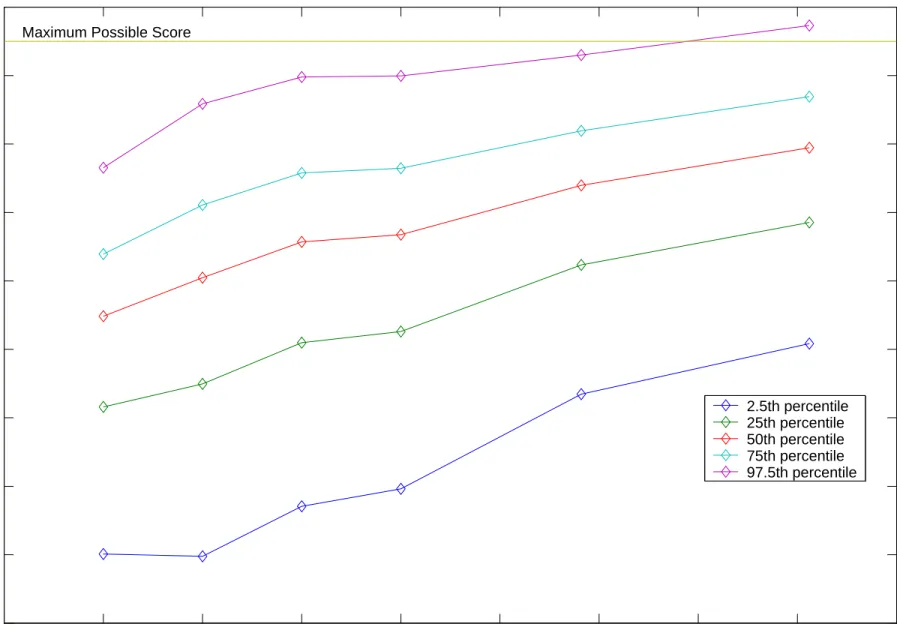
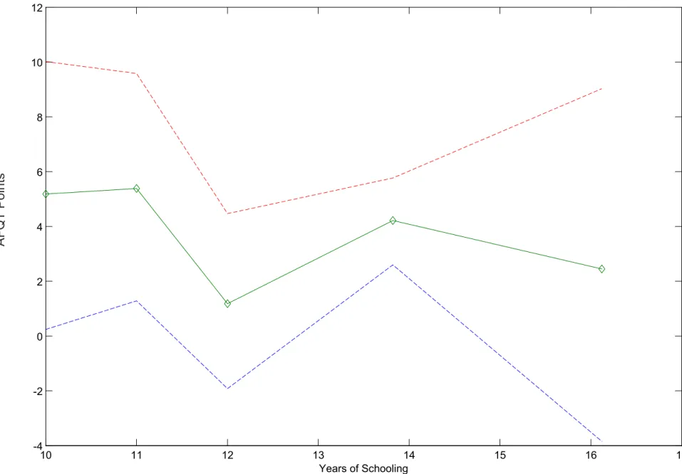
Wefirst discuss thefit of the estimated model to the data. Tables 7 and 8 describe thefit of the model to the data for the schooling choice and test systems, respectively. The fit reported in Table 7 is quite good both overall and in partitions of the data on selected covariates. Figures 1(a)-(f) plot the fitted AFQT
33In addition to the covariates above we included a dummy variable in the test score equations for having completed
strictly less than 9 years of school to allow for possible heterogeneity in the grade school and ninth grade composite group; the coefficient on this dummy was insignificant for all tests.
test score distribution against the actual empirical CDF for each schooling group. We passχ2 goodness of
fit tests at conventional levels of significance for most groups though the figures reveal a slight tendency to underpredict scores for the lowest schooling category and to overpredict test scores for the highest two schooling groups. The goodness of fit statistics are reported in Table 8. The fit is worst for the most heterogeneous groups, “ninth grade or less” and “some college.” In fact, the poorfit in the “some college” category causes us to fail the overall test of fit.34 Excluding that group we would pass the overall test.
5.2.2 Estimated Cognitive Ability Distribution
Figure 2 displays the estimated latent ability or factor distribution plotted against “residualized AFQT” (constructed by running an ordinary least squares regression of standardized AFQT score on family background and cohort dummies). Recall that the location and scale of the latent ability distribution must be set since they are not identified in the model. This is a standard result in factor analysis. Recall that we set the location by constraining the unconditional mean of the factor to be zero (note the residualized AFQT distribution also has mean zero by construction). The scale is set by a normalization in one of the test score equations. Specifically, we set to 1 the coefficient on the factor in the equation for the Word Knowledge test component (standardized to have within-sample mean 0 and variance 1) estimated for individuals who had completed eleven years of schooling at the test date.35
The estimated factor density is not normal and closely tracks but does not completely resemble the conventional residualized AFQT density. Residualized AFQT computed by OLS (not accounting for schooling or selection effects) is an imperfect measure of cognitive ability. While the mean of the factor is
fixed to0, the estimated median, 0.1158,is positive, so that more than half of the population has above average ability. However the estimated range of the factor distribution is skewed negative: a person who is at the 2.5th percentile in ability is more than half a standard deviation further away from the average (at−1.4846) than a person at the 97.5th percentile (with ability1.1131).
5.2.3 Allowing for Age and Endogenous Entry Dates
By using the sampleS =ST, we break the dependence betweenA andN given by (14). We parameterize
age effects on test scores by assuming
λ(A, S) = λ(S)36
µ(A, S) = β1(S)A+β2(S)
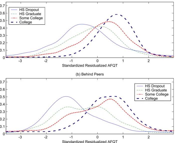
whereβ1(S)andβ2(S)are unrestricted functions ofS. In this paper we explicitly model the relationship between entry date N and latent ability f. The model specifies a jointS×N space. How important is it to account for endogeneity of N ? Figure 3 plots the distributions of latent ability f conditional on entry statusN. Note that individuals who are behind their peers on average have lower latent ability than their
34TheP value for the overallfit of the model excluding some college is0.1050. 35The estimated standard deviation of the factor is0.7027.