Probabilistic Estimation of Unmarked Roads using
Radar
Juan I. Nieto, Andres Hernandez-Gutierrez and Eduardo Nebot
Abstract—This paper presents a probabilistic framework for unmarked roads estimation using radar sensors. The algorithm models the sensor likelihood function as a Gaussian mixture model. This sensor likelihood is used in a Bayesian approach to estimate the road edges probability distribution. A particle filter is used as the fusion mechanism to obtain posterior estimates of the road’s parameters. The main applications of the approach presented are autonomous navigation and driver assistance. The use of radar permits the system to work even under difficult environmental conditions. Experimental results with data acquired in a mine environment are presented. By using a GPS mounted on the test vehicle, the algorithm outcome is registered with a satellite image of the experimental place. The registration allows to perform a qualitative analysis of the algorithm results. The results show the effectiveness of the algorithm presented.
Index Terms—Localisation, radar sensors, particle filter I. INTRODUCTION
O
NE of the most important tasks in autonomous naviga-tion is the segmentanaviga-tion of the road course [1], [2]. The design of a robust road estimation system needs to consider variations among roads such as paved or unpaved, marked or unmarked. Roads in urban environments have in general well defined lane marks, constant width and well defined corners. On the other hand, roads in rural areas tend to have much less structure and are in general unmarked. Mining roads are a good example of the later. Roads in mines are unpaved, no lane markers are presented, and a constant variation of the road width can be found. The lack of structure in rural areas makes the vehicle relative positioning process harder.Road estimation is not only important for autonomous navigation but it can also be utilised for driver assistance systems [3]. An example of a warning system aiming driver assistance in unmarked roads is presented in [4]. The system estimates the relative vehicle position using range information gathered from a laser scanner. The range data is used to measure the relative distance between the vehicle and poles located at the side of the road. The additional infrastructure added on side of the road ensures the system can reliably detect when a vehicle gets too close to the center or side of the road. The main disadvantage of the system is the need for installation and maintenance of infrastructure (poles at the side of the roads).
The design of a road estimation system will also depend on the sensors selected. Radar sensors have proven to be very robust to different weather conditions such as dust,
Juan I. Nieto, Andres Hernandez-Gutierrez and Eduardo Nebot are with the Australian Center for Field Robotics at the University of Sydney. E-mail: {j.nieto,a.hernandez,nebot}@acfr.usyd.edu.au
fog and snow. These positive aspects have encouraged car manufactures to equip vehicles with radar sensors to perform intelligent tasks, such as collision avoidance, traffic scene interpretation and moving objects detection. However, radar based navigation systems are seldom used to provide infor-mation related to vehicle position relative to road edges. This is due to the cost of the technology and also partly to the difficulty in processing the information returned. For example, due to the wider beam pattern, radar information from a given bearing will in general consist of various returns at different ranges. At the same time objects with large radar target that are not within the nominal current bearing cone could potentially generate an erroneous return at the present bearing. These issues with radar add an extra complexity and therefore this sensor modality is usually avoided when not specifically needed. In most applications vehicles are equipped with other sensors modalities for road shape estimation, such as cameras and laser scanners. For instance, vision systems are well suited to detect lane markings. Laser scanners have high resolution in azimuth and wide field of view which makes them suitable for the extraction of berms and curves along the edges of the road. The main disadvantage of visual and laser sensors is the lack of robustness against bad weather conditions such as fog and dust for example.
The work presented in this paper aims to develop a system to work in unpaved and unmarked roads and under harsh environ-mental conditions. This is the case for example of autonomous operation in a mine where the system needs to operate reliable 24/7 under all environmental conditions. The harsh conditions requirement restricts the choices of possible sensors, being radar the most suitable one. For this type of applications, the radar becomes an essential component to enable automation and operator aiding. The algorithm presented in this work performs Bayesian estimation of the road’s edges which allows to obtain the probability distributions of the road parameters and vehicle relative position. The system is robust to sensor noise since incorporates the uncertainty in a Gaussian mixture likelihood function.
This paper is organized as follows. Section II presents related work. An overview of the algorithm is described in section III. Section IV shows the model to represent the road. The algorithm proposed using particle filters is explained in section V. Information related to the radar sensors as well as GPS positioning is detailed in Section VI followed by experimental results in Section VII. Conclusions and future work are presented in Section VIII.
II. RELATEDWORK
Several approaches for road tracking have been proposed during the last two decades. These works have emerged as a need of intelligent transportation systems for an everyday crowded world. Vision-based road tracking systems are pre-sented in [5], [6] and [7]. The system described in [5] estimates the curvature and orientation of a road based on monocular frames and a model of the road. First, the algorithm segments the acquired images to extract road edges and orientation. In order to remove outliers, the least median squares filter is applied. Using inverse perspective projection, feature points in the image are projected back onto the ground plane and the coordinates of the marking lanes, relative to the camera are computed. This technique works efficiently for marked roads. In contrast, [7] presents an approach that deals with both marked and unmarked roads using a monochromatic camera. Applying a statistical model, this method copes with problems such as occlusion and not well defined marks. Besides the lane detection and tracking estimation, this algorithm also estimates the vehicle position within the road. The approach presented in [8] is based on the extended Kalman filter and a linear model to estimate and track successively the road curbs. This method works well when curbs are well defined.
In addition to mono-sensor approaches, algorithms that im-prove robustness by fusing information from different sensors modalities have been proposed in [9] and [10]. In [9], the detection of curbs and walls are based on a laser scanner, a GPS device, an inertial measurement unit (IMU) and a monochromatic camera. This system is capable of detecting curbs alongside the vehicle and at the front. Our work is more related to the framework shown in [10], where the authors present a technique that integrates information gathered by optical and radar imaging sensors. By using deformable tem-plate models of lane and pavement boundaries together with likelihood models of the sensors, the detection and tracking of lane and pavement boundaries are implemented in a Bayesian framework. The work presented here is based on radar only.
III. ALGORITHMOVERVIEW
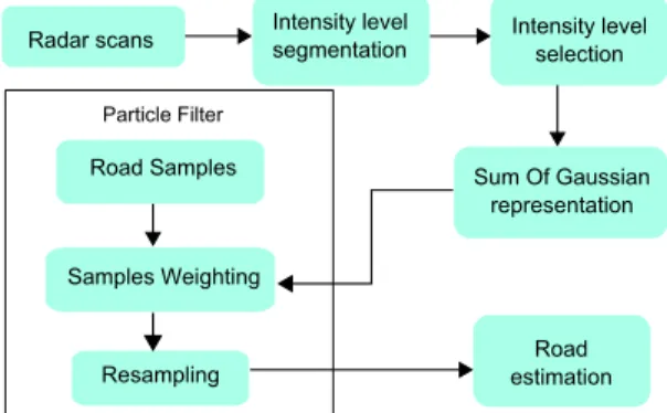
In this paper we present a probabilistic road estimation system to evaluate both the width of the road, and the vehicle position with respect to the road’s edges. The proposed method is based on information gathered by a millimetre-wave radar that detects salient points located around the vehicle. The sensor’s returns are segmented into different intensity levels. Sensor data is then modeled as a Gaussian Mixture Model (GMM) as the uncertainty associated to each intensity level of each particular radar bearing return is modeled as a Gaussian. Monte-Carlo sampling is used to geta-prioriestimates of the road. The system uses Clothoid functions defined over a set of parameters to model the road shape. Once road samples are obtained, they are fused with the likelihood GMM built with the observations. The fusion is done using a particle filter, which weights the road samples according to its probabilities. As a result, the system provides a stochastic road’s shape model. Figure 1 presents a block diagram of the framework.
Resampling Particle Filter Road Samples
Samples Weighting
Radar scans Intensity levelsegmentation Intensity levelselection
Sum Of Gaussian representation
Road estimation
Fig. 1. Block diagram of the proposed method to estimate the shape of the road using radar information.
IV. ROADMODEL
Clothoids functions are widely used for road design in order to connect geometry between a straight line and a circular curve. The main characteristic of a Clothoid curve is that the curvature is proportional to the inverse of the radius. The Clothoid’s geometry models well the centripetal acceleration experienced by a vehicle approaching a curve.
To model the road ahead of the vehicle, we use a polynomial cubic approximation of a Clothoid [11]
y(x) =y0+tan(φ)x+C0 x2
2 +C1
x3
6 (1)
wherey is the distance between the vehicle and the proposed left road, beingy0 the initial offset. The orientation angle of
the road relative to the vehicle coordinate frame is given byφ.
C0 andC1 represent the curvature and curvature rate
respec-tively. Figure 2 illustrates the model described in Equation 1. Although the width of the roadW is not included in Equation 1, this parameter will be also estimated as it will be shown in Section V-A. x y y(x) y0 �
Fig. 2. Model of the road using a Clothoid function.
V. ROADESTIMATION USINGPARTICLEFILTERS
Particle filters are a recursive Bayesian estimation tool based on Monte Carlo sampling methods. Unlike the Kalman filter, particle filters have the advantage of not being subjects to any linearity or Gaussianity constraint on both the transition and observation model [12], [13]. The basic idea behind particle filters is to represent probability distributions by a set of random samples or particles. In order to make inference about a dynamic process, particle filters usually use two models; a state evolution model and an observation model, being both
models perturbed by noise. The filter is articulated through two main steps, prediction and update. During the prediction stage, particles representing random samples of the estimated states are passed through the system model. During the update stage, the new measurements received are used to update the likelihood of the prior samples and obtain normalised weights for the samples. The weights represent the likelihood of the model encapsulated by the individual particles [14].
The particle filter implemented here is the Condensation algorithm, presented in [15] for tracking curves in visual clutter. The state vector is represented by the parameters used to model the Clothoid, shown in Equation 1 plus the road width W.
x= [Y, φ, C0, C1, W]T (2) A. Process Model
The vehicle model is approximated by the Ackerman bicycle model ˙ x ˙ y = v(t)cosθ v(t)sinθ (3) Fusing Equation 1, which represents the shape of the road, with the vehicle model described in Equation 3, the state evolution model can be obtained.
Yt+1 θt+1 C0t+1 C1t+1 Wt+1 =A(∆s) Yt θt C0t C1t Wt + 0 −∆θt 0 0 0 +w(t) (4) A(∆s) = 1 ∆s ∆s2 2 ∆s3 6 0 0 1 ∆s ∆2s2 0 0 0 1 ∆s 0 0 0 0 0.99 0 0 0 0 0 1 (5)
where Y represents the distance between the vehicle and the proposed road. φ is the orientation angle of the road with respect to the vehicle location. C0, C1 and W are the
curvature, rate of curvature and width of the proposed road.
∆s represents the longitudinal displacement along the curve from timettot+1andw(t)the process noise, which is a zero-mean white noise sequence. The vehicle speed involved in (3) as well as its longitudinal displacement, which is represented by∆sin (5), are provided by the GPS receiver. Figure 3 shows an example of road samples superimposed on a satellite image.
B. Sensor Likelihood Function
We assume the sensor possesses normally distributed noise. Thus, a radar scan can be represented as a Gaussian Mixture Model (GMM). Radar returns are originally in polar coordi-nates, being described by range r and bearingθ information. For the road estimation process, data is converted from polar to Cartesian coordinates that is the space we are interested.
Fig. 3. The red curves in the figure illustrates the road samples using the Clothoids model. Yellow points denote the selected radar returns and blue dots the GPS trajectory.
fx,y(r, θ) = r cosθ r sinθ (6) The sensor information is considered to be uncorrelated in the original polar space, therefore the covariance matrix associated to a radar return can be represented as
Σr,θ = σ2r 0 0 σ2 θ (7) The covariance matrix in Cartesian coordinates is obtained through a linearisation of Equation 6.
Σx,y =J Σr,θ JT (8) whereJ is the Jacobian offx,y(r, θ)andΣr,θis the covariance matrix associated to the radar data as in (7). Figure 4 depicts an example of a GMM representing a radar scan. As seen in this figure, the edges of the road can be well defined by the Gaussians. −30 −20 −10 0 10 20 30 −20 −10 0 10 20 0 1 2 3 x−axis [m] y−axis [m] sum of Gaussians
Fig. 4. GMM representing a radar scan.
C. Model Update
The prediction stage gives a set of particles, each represent-ing a different set of road parameters. In order to decide which proposed road better describes the shape of the road, we use an objective function to weight each particle according to the
likelihood obtained using the GMM sensor model. Firstly, the left and right proposed roads are discretised and evaluated in the sum of Gaussian map as follows
clsi =X k∈P Lk (9) cris=X k∈P Rk (10)
where Lk and Rk are the Gaussian values along the left and right proposed roads. The total cost for a proposed road,
xsi ∈Xs, is given by the sum of these individual distances as follows
Cis=clsi +crsi (11) This cost value will be used by the particle filter to weight each particle.
Using the total cost associated to each of the proposed roads, the particles are weighted by applying the following expression
wit = Cis P i∈S C s i (12) wherewit is theithweight of the proposed road at timet,
andN the number of particles.
D. Resampling
An important drawback of particle filters is the so called
degeneracy problem. The degeneracy problem is when most particles have weights very close to zero therefore only few samples are being used to represent the distribution. Resampling is used to avoid this problem by selecting and multiplying the most “important” particles (biggest weights) and eliminating the particles with the lowest weights. In other words, the resampling process selects the set of particles that best represents the distribution. The filter implemented here is a sampling importance resampling (SIR) as presented in [14] and [15] and uses Stratified resampling [16].
VI. SENSORS
The main objective of road estimation is vehicle relative positioning and so global position estimation is not needed. However, due to the difficulties arising in attempting to get ground truth of the relative position to the road, a quantitative analysis of the results is not possible and instead we provide a qualitative analysis by superimposing the vehicle trajectory and estimated road with a satellite image. A GPS sensor mounted on the experimental vehicle is used to get position estimation. The data was gathered in a mine, with the sensors mounted on a truck. Sensors’ details are presented next.
A. GPS Data
The GPS used for this work is a standard A12 from Thales Navigation, working in autonomous mode which gives and accuracy between 2 and 10m. Information such as latitude, longitude, heading and speed of the vehicle is available every second.
B. Radar Data
External information is acquired by a radar scanner working at 94 GHz [17]. The radar has an uncertainty of 20cmin range and1degin angle. The radar returns different intensity values. In order to convert from intensity to range, we use a linear model
r=Ab−C (13)
wherer is the range from the radar return, A represents the radar resolution, that in this case is23.52cm bin−1,b is the
bin number for the return and C is the offset between the transmitter and the receiver in the radar, which is60 cmfor this sensor. Figure 5 shows an example of intensity return versus bin values for a particular angle. This radar scan was acquired at 33 deg. In this case, the maximum intensity value, 94.99dB, corresponds to an object located at bin 63; therefore, the range to this object is 21.744 m.
0 50 100 150 200 250 300 0 10 20 30 40 50 60 70 80 90 100 X: 63 Y: 94.99 bins intensity [db]
Fig. 5. Reflectivity values scattered by objects located at a given rotation angle of the radar. Range is discretized into bins with0.2353mresolution. For an object found at bin 63 having an intensity of94.99dB, its range will be21.744m.
For the work presented, we limited the radar data to 200 bins, that represents a maximum range of approximately46m. This range was enough to detect the road boundaries. Because we are interested in detecting the edges which in general reflect large intensity values, we use thresholds to select the largest intensity values and segment each return into a discrete number of ranges. The different intensity values correspond to reflections from objects that are at different distances to the sensor. In the results presented here we use thresholds at 51dB, 71dB,76dB, 80dB and 82dB. These values were obtained through experimentation. It is important to note that the segmentation is mainly used to reduce the amount of data. We did not find the threshold values to be an important factor in our implementation as long as the values with the highest intensities were included.
Figure 6 depicts an example of the segmentation process, superimposed on a satellite image. Objects represented by blue and green points reflect back an intensity value greater than
the first and second thresholds; whereas objects represented by yellow, red and violet points have an intensity value greater than the third, fourth and fifth thresholds respectively. In order to filter out radar information corresponding to the roof of the vehicle, data located within a range of 2.5 m is removed. This is represented in the figure with a small circle around the sensor position.
Fig. 6. Reflectivity values segmented into five different levels. Intensity values represented by green points are considered in the road shape estimation; whereas, points in blue are removed. GPS position is represented by blue dots along the trajectory.
VII. EXPERIMENTALRESULTS
The experimental data was collected in a mine, in southeast Queensland, Australia. A millimetre radar (94 GHz) was mounted on top of the experimental vehicle. The whole vehicle trajectory was around 1.5km.
Figure 7 displays an image of the experimental area, together with the vehicle trajectory, radar returns and road estimates. Yellow points represent the targets detected by the radar sensor along the trajectory. As can be seen in the figure, high intensity values are returned not only from the edges of the road, but also from the trees, obstacles located around the path and also there are high intensity returns from within the road. The large amount of data and the noise included in the sensor returns make the road estimation a very difficult problem. The vehicle position reported by the GPS device is illustrated in blue dots within the path.
The red lines showed in Figure 7 show the final left and right road edges estimated. The filter was run using 500 particles. As shown in Figure 7, the estimated edges define appropriately the edges of the road along the trajectory. Note that part of the offset observed with the satellite image is due to the error in GPS position which is used to register the radar points with the image.
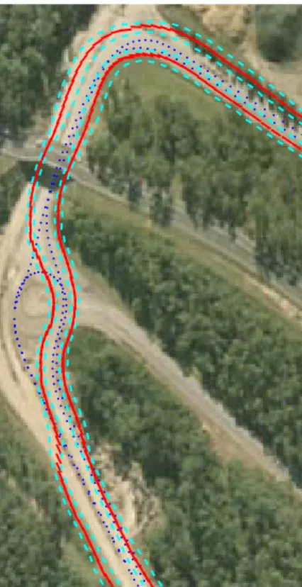
Figures 8 and 9 show a zoom-in of the estimated road edges together with their uncertainty obtained from the particle fil-ters. The dashed lines represent the ±2σuncertainty obtained from the samples variance. As seen in Figure 8, the actual road’s edges are found within the uncertainty area. Note that the uncertainty in the first curve (Figure 8 bottom part), is bigger than the one near the bridge (Figure 8 top-left). This
Fig. 7. Estimated edges of the road and radar data superimposed on the satellite view. The edges and the centre-line of the road are represented by the red and green line respectively; whereas, the vehicle position is illustrated by blue dots along the trajectory.
is because the area near the bridge presents a higher density of points, which gives a better road estimate. See also the area around the roundabout, where the edges are very poorly defined. Although in this area the sensor returns very little information about the edges, the algorithm is still able to get good estimates.
Figure 9 shows a zoom-in of the trajectory center area. In this figure, the actual road’s edges are also found within the uncertainty area. The area near the bottom part of the trajectory presents a larger error. This is due to the large amount of returns coming from trees that introduce extra uncertainty in the road estimation process.
Figure 10 shows the width of the road along the complete trajectory. This parameter varies from 11.5m to 28m corre-sponding the first of these values to the trajectory around the roundabout as shown in Figure 8. The width starts increasing when the vehicle is being driven through the wide curve shown in Figure 9.
Finally, Figure 11 displays the distance between the vehicle position and the left edge of the road. The small values are presented when the vehicle is turning to the left at the first curve and after passing the roundabout in Figure 8.
VIII. CONCLUSIONS ANDFUTUREWORK
This paper presented a probabilistic approach for road extraction using radar data. Radar information is modelled
Fig. 8. Estimated edges of the road describing the first and second curve located in the top left corner in Figure 7 along with the uncertainty area represented by cyan dashed lines. This area represents±2σof the estimated roads.
Fig. 9. Estimated edges of the road describing the third curve found in Figure 7 along with the uncertainty area represented by cyan dashed lines. This area represents±2σof the estimated roads.
0 50 100 150 200 250 300 10 12 14 16 18 20 22 24 26 28 30 scan number
width of the road [m]
Fig. 10. Road width along the driven trajectory. The width varies between 12mand28m. These two values correspond to the width estimated along the roundabout in Figure 8 and the curve in Figure 9.
0 50 100 150 200 250 300 0 2 4 6 8 10 12 scan number
offset between the vehicle and the left edge of the road [m]
Fig. 11. Distance between the vehicle and the left edge of the road. The small values occur when the vehicle is turning to the left and passing the roundabout.
as Gaussian Mixture Models (GMM) where the uncertainty associated to each radar return was considered. A polynomial cubic approximation of a Clothoid function was applied to model the shape of the road. These clothoid functions were evaluated in the GMM, so that it was possible to compute the total cost for each proposed road.
Experimental results with data acquire in a mine environ-ment validated the approach. A qualitative analysis of the results was done by superimposing the filter output on a satellite image. The good results obtained are very encouraging considering that no special work (such as adding infrastruc-ture) was performed on the berms limiting the road. This implies that results could be improved by proper maintenance of the road. A system like the one presented will be essential for operator aiding under difficult environmental conditions or autonomous operations.
Future work will include the fusion of radar data with vision. The rich information provided by a visual sensor,
such as texture and colour will facilitate road discrimination, principally in clutter areas where the radar data is difficult to interpret. Furthermore, by using visual sensors such as stereo cameras, it is possible to recover the 3D structure of the environment, thus, an interpretation of the terrain could be obtained.
ACKNOWLEDGMENTS
We would like to thank to Graham Brooker and Javier Martinez from the Australian Centre for Field Robotics for providing the radar data and their help and support with the data processing.
This work has been partially supported by CONACYT and SEP Mexico, the ARC Centre of Excellence programme, funded by the Australian Research Council (ARC) and the New South Wales State Government.
REFERENCES
[1] S. Thrun and et.al, “Stanley: The robot that won the darpa grand challenge,”Journal of Field Robotics, vol. 23, no. 9, pp. 661–692, 2006. [2] P. Beeson, J. O’Quin, B. Gillan, T. Nimmagadda, M. Ristroph, D. Li, and P. Stone, “Multiagent interactions in urban driving,”
Journal of Physical Agents, vol. 2, no. 1, 2008. [Online]. Available:
http://www.jopha.net/index.php/jopha/article/view/14/13
[3] R. Risack, P. Klausmann, and W. Kruger, “Robust lane recognition embedded in a real-time driver assistance system,” inIEEE International
Conference on Intelligent Vehicles, Jan 1998, pp. 35–40.
[4] E. Nebot, J. Guivant, and S. Worrall, “Haul truck alignment monitoring and operator warning system.””Journal of Field Robotics”, vol. 23, pp. 141–161, 2006.
[5] K. Kluge, “Extracting road curvature and orientation from image edge points without perceptual grouping into features,” in Proceedings of
Intelligent Vehicles Symposium, 1994, pp. 109–114.
[6] K. Kluge and C. Thorpe, “The yarf system for vision-based road following.””Mathematical and Computer Modelling”, vol. 22, pp. 213– 233, Aug 1995.
[7] R. Aufrere, R. Chapuis, and F. Chausse, “A fast and robust vision based road following algorithm,” inProceedings of Intelligent Vehicles
Symposium, 2000, pp. 192–197.
[8] W. Wijesoma, K. Kodagoda, and A. P. Balasuriya, “Road boundary detection and tracking using ladar.”IEEE Transaction on Robotics and
Automation, vol. 20, pp. 456–464, Jun 2004.
[9] R. Aufrere, C. Mertz, and C. Thorpe, “Multiple sensor fusion for detecting location of curbs, walls, and barriers,” in Proceedings of
Intelligent Vehicles Symposium, 2003, pp. 126–131.
[10] B. Ma, S. Lakshmanan, and A. O. Hero, “Simultaneous detection of lane and pavement boundaries using model-based multisensor fusion.”IEEE
Transaction on Intelligent Transportation Systems, vol. 1, pp. 135–147,
2000.
[11] R. Lamm, B. Psarianos, and T. Mailaender,Highway design and traffic
safety engineering handbook. McGraw-Hill, 1999.
[12] B. Southall and C. J. Taylor, “Stochastic road shape estimation,” inICCV
Eighth International Conference on Computer Vision, 2001.
[13] B. Ristic, S. Arulampalam, and N. Gordon,Beyond the Kalman Filter:
Particle Filters for Tracking Applications. Artech House, 2004.
[14] N. J. Gordon, D. J. Salmond, and A. F. M. Simth, “Novel approach to nonlinear/non-gaussian bayesian state estimation,” IEE Proceedings-F, vol. 140, no. 2, pp. 107–113, Apr. 1993.
[15] M. Isard and A. Blake, “Icondensation:unifying low-level and high-level tracking in a stochastic framework,” inECCV European Conference of
Computer Vision, 1998.
[16] G. Kitagawa, “Monte carlo filter and smoother for gaussian non-linear state space models,” Journal of Computational and Graphical Statistics, vol. 5, no. 1, pp. 1–25, 1996.
[17] G. Brooker, “Understanding millimetre wave fmcw radars,” in