T
HE
W
ILLIAM
D
AVIDSON
I
NSTITUTE
AT THE UNIVERSITY OF MICHIGAN BUSINESS SCHOOLThe Balassa
-Samuelson Effect in Centra
l
and Eastern Europe: Myth or Reality?
By: Balázs Égert, Imed Drine, Kirsten Lommatzsch
and Christophe Rault
William Davidson Working Paper Number 483
July 2002
The Balassa-Samuelson effect in Central and Eastern
Europe: Myth or reality?
A panel study
Balázs Égert1
MODEM, University of Paris X - Nanterre
Imed Drine
EUREQua, University of Paris I - Sorbonne
Kirsten Lommatzsch
German Institute of Economic Research, Berlin
Christophe Rault
EUREQua, University of Paris I - Sorbonne ABSTRACT:
This paper studies the Balassa-Samuelson effect in 9 CEECs . Using panel cointegration techniques, we find strong empirical evidence in favour of what we call the internal transmission mechanism since productivity growth in the open sector is found to bring about non-tradable inflation. However, we also shed new light on the fact that the impact of the internal transmission mechanism on overall inflation is considerably attenuated by the low share of non-tradables in the consumer price index. Furthermore, we argue that because of this and the high share of food items and regulated prices, the CPI may be misleading when analysing the Balassa-Samuelson effect. The paper also shows that the appreciation of the transition economies’ real exchange rate, which has become something of a stylised fact over the last decade is only partly caused not the Balassa-Samuelson effect. Instead, we argue that a trend increase in tradable prices is behind this phenomenon.
Key Words : Balassa-Samuelson effect, Panel cointegration, Transition economies, EMU
JEL Classification : E31, F31,C15.
1 Corresponding author, MODEM, University of Paris X - Nanterre, bât G, 200, avenue de la République, 92001–
1. Introduction
The near EU-accession of CEE countries has provoked a substantial debate on when and how new entrants should adopt the euro. As they are not granted an opt-out clause from EMU, after entering the EU, new entrants are supposed to strive for achieving nominal convergence in accordance with the Maastricht criteria. It is a widely held view that this might be in conflict with the aim of real convergence. In particular, it is maintained that it may be difficult to meet simultaneously the Maastricht criterion on inflation and that on exchange rate stability in the framework of ERM II (Cf. Kopits 1999, Corker et al. 2000, Szapáry 2000, Halpern/Wyplosz 2001, Buiter/Grafe 2002).
According to the Balassa-Samuelson effect (Balassa 1994, Samuelson 1964) on which this professional wisdom is based, productivity growth in the open sector usually exceeds that in the sheltered sector. Given that wages are expected to be approximately the same across sectors, faster productivity growth in the open sector pushes up wages in all sectors, thus leading to an increase in the relative prices of non-tradable goods. Therefore, if productivity growth in one country outpaces that in the other, overall inflation will be higher in the former. In the case of the accession countries, such inflation differentials will be a source of price level convergence vis-à-vis EU countries and will also affect the CPI calculated real exchange rate. In fact, as long as the nominal exchange rate is determined by PPP in the open goods, a productivity induced increase in the price level through relative price adjustments will result in an appreciation of the CPI based real exchange rate.
The Balassa-Samuelson effect can expected to be at work in CEE countries. After the initial recession, these countries have experienced rapid (productivity) growth in particular in their industrial sectors going in tandem with a steady increase in the relative price of non-tradables and a trend appreciation in the real exchange rate. Nevertheless, there is still ample room for further productivity and price level convergence (cf. Eurostat (2001a)). The conflict between nominal and real convergence could arise, because with a fixed exchange rate relative price adjustments can only take place through non-tradable inflation. By contrast, relative price adjustments can be achieved without inflation in the presence of floating exchange rates as a nominal exchange rate appreciation will imply declining tradable prices measured in domestic currency terms. Therefore, with strong catch-up in the accession countries productivities, this raises doubts as to whether the inflation and the exchange rate targets could be simultaneously achieved.
There is a fast growing empirical literature on transition economies concentrating both on relative price and real exchange rate developments attributable to the Balassa-Samuelson effect. Whereas the existence of a long-run relationship between non-tradable inflation and productivity growth is broadly
acknowledged, estimations concerning the extent to which the Balassa-Samuelson effect is reflected in inflation differentials and consequently in real exchange rate movements differ considerably. Some estimates, e.g. by Kovács/Simon (1998), Rother (2000), and Halpern/Wyplosz (2001) show that productivity driven real appreciation is approximately 3 per cent per annum in a number of transition economies. By contrast, De Broeck - Slok (2001), Corricelli - Jazbec (2001) and Égert (2002a,b) are much more cautious about the magnitude of the Balassa-Samuelson effect as it is likely to justify a real appreciation ranging from 0% to 1.5% a year.
This paper contributes to this debate on transition economies by investigating the Balassa-Samuelson effect for 9 CEE transition countries using detailed national accounts data for productivity and relative price measures. We use different classifications for the open and the sheltered sector. The investigated period ranges from 1995 to 2000 since we eliminated the early years of transition, during which price and productivity developments were much more driven by the initial reforms rather than by the Balassa-Samuelson effect itself. Using panel cointegration methods, we find that productivity growth in the traded goods sector is likely to bring about non-tradable inflation. However, this does not mean that productivity gains will be automatically reflected in overall inflation and thus in an appreciation of the real exchange rate. Actually, the impact of productivity on inflation depends chiefly on the composition of the consumer basket. When the weight of non-tradables is low, increases in relative prices will have little impact on overall inflation. The issue of regulated prices should also be addressed, as they are expected to have a non negligible share in non-tradable items in the CPI. Whilst increases in regulated prices seem to accentuate the Balassa-Samuelson effect, what really matters is the share of market-based non-tradables in the CPI. Furthermore, the tradable good price-deflated real exchange rate also trend-appreciates in those countries implying that PPP does not hold in the open sector. A consequence of the persistent tradable price inflation differential is that the conflict between nominal and real convergence related to the Balassa-Samuelson effect may be weaker than shown before. We conclude that other factors of the price convergence process, in particular the convergence in traded good’s prices, should be examined in more detail.
The remainder of the paper is organised as follows: Section 2 briefly discusses the theoretical framework. Sections 3 subsequently describes the relationships between productivity, relative prices and real exchange rates we derive from the model. In the following two sections, data and econometric techniques employed in this study are presented. Section 6 gives an overview of the results. Section 7 finally concludes.
2. The Balassa-Samuelson model
The Balassa-Samuelson model provides a supply side explanation for the relative price of tradables and non-tradables in an economy, and, assuming that PPP holds for traded goods, for differences in price levels between countries with different levels of development and for the long-run behaviour of the consumer price deflated real exchange rate. To establish that the relative price of non-tradables and tradables and thus the price level composed of tradable and non-tradable goods is entirely determined by the supply conditions, i.e. the production functions of an economy, a number of assumptions have to be made:
- each economy produces two kinds of goods with two different constant-return-to-scale Cobb-Douglas production functions:
(1)
Y
t=
A
t⋅
L
bt⋅
K
t(1−b) (2)Y
nt=
A
nt⋅
L
cnt⋅
K
nt(1−c)where Y, L, K, A stand for output, labour, capital and total factor productivity. “t” and “nt” denote variables in the traded and the non-traded goods sector, respectively, and 0 < b < 1 and 0 < c < 1. - the labour elasticity of production is larger in the non-traded goods sector than in the traded goods
sector (c > b)
- the prices of tradable goods are determined in the world market (i.e. they are exogenous to the model), - the interest rate is determined in the world market
- capital stock is fixed for one period ahead
- labour is perfectly mobile across sectors, but less mobile at an international level
- real wages in the traded goods sector are determined by the marginal product, and because of the wage equalisation process in the economy, the nominal wages paid in the traded goods sector also hold for the non-traded goods sector2.
If these assumptions hold, the relative price of non-tradable goods can then be solely determined by the supply conditions. This follows from the first-order conditions of the profit maximisation problem of producers of tradable and non-tradable goods and the assumed exogeneity of the mentioned variables. The first-order conditions are the following using Cobb-Douglas production functions:
(3)
( )
t b nt t tp
i
L
K
b
A
=
⋅
−
⋅
1
1
2 In response to one of the referees comment, we would like to clarify that marginal productivity in the non-traded
(4) t b t t t p W L K b A ⋅ ⋅ = − ) 1 ( (5) nt c nt nt nt p W L K c A = ⋅ ⋅ (1−) (6)
( )
nt c nt nt ntp
i
L
K
c
A
=
⋅
−
⋅
1
1
where W, P and i denote wages, prices and interest rate.
The four endogenous variables in this model are determined as follows: the only unknown variable in Equation 1 is labour input for the traded goods sector. Therefore, the interest rate and the capital stock determine the capital-labour ratio, and consequently the labour input for the tradable sector. Equation 2 determines the nominal wage in the tradable sector, which enters as exogenous in the first-order conditions for the tradable sector. The third and fourth equations jointly determine labour input in the non-tradable sector and the (relative) price of the non-non-tradable. Hence, the relative price of the non-non-tradable goods is solely given by the supply conditions, and reflects a microeconomic equilibrium.
If productivity advances in the tradable sector exceed those in the non-tradable sector, a country will experience a rising price level brought about by an increase in the relative price of non-tradable goods. This is quite probable, as capital intensity is assumed to be higher in the tradable sector. Owing to the assumption that tradable prices are determined in the world market, productivity advances in the traded goods sector do not have any impact on tradable price developments. Nevertheless, wages can rise at a proportional rate in the open sector without harming competitiveness. Since wages equalise across the open and sheltered sector, a rise in the wage level induces an increase in wages in the sheltered sector, and, in the absence of any corresponding improvements in productivity in the latter sector, this will lead to an increase in non-tradable prices. As a result, productivity gains in the open sector will bring about overall inflation through the rise in non-tradable prices. This can be referred to as the internal transmission mechanism from productivity growth in the tradables sector towards non-tradable prices and overall inflation.
Let us now consider the differences in price levels and price developments between countries at a different stage of economic development. According to the Balassa-Samuelson model, differences in the traded goods sectors’ productivities and consequently the wage level are at the root of different price levels
determine the amount of labour employed in this sector, wages in the non-traded sector will also equal the marginal product in this sector as well.
between economies with different levels of development. This is caused by the fact that differences in price levels are entirely determined by differences in non-tradables prices assuming PPP holds for tradable goods. At the same time, the catch-up process, i.e. when less developed countries experience faster productivity growth than the more developed economies especially in their traded goods sector, is accompanied by an increase in the relative price of non-tradables within the economy and a trend appreciation of the real exchange rate calculated using the CPI. This is the reason why the Balassa-Samuelson model also functions as a model for long-term real exchange rate determination. Deviations from PPP occur if the productivities in the traded goods sector and thus the prices of non-traded goods differ. The catch-up process entails a real appreciation, which is – in accordance with the internal mechanism – determined by a microeconomic equilibrium process. Therefore real appreciation caused by the Balassa-Samuelson effect cannot be avoided, as it reflects rising productivity. Furthermore, this type of real appreciation does not harm a country’s competitiveness, because tradable prices do not change.
3. Testable equations
The internal transmission mechanism suggests that the differential between productivity in the open and the sheltered sector and the relative price of non-tradable goods compared to that of tradable goods should be connected. This relationship can be derived from the order conditions. Equating wages in the first-order conditions determining labour input leads to equation (7):
(7) nt nt t t t nt
L
Y
L
Y
P
P
∂
∂
∂
∂
=
Hence an increase in the relative price of non-tradables occurs when productivity increases faster in the tradable sector than in the non-tradable sector. This can be easily proved, if marginal productivity can be approximated by average productivity. When using Cobb-Douglas production functions, such an approximation can be given as follows:
(8) t t b t t t t t
L
Y
b
L
K
b
A
L
Y
⋅
=
⋅
⋅
=
∂
∂
1− and (9) nt nt c nt nt nt nt ntL
Y
c
L
K
c
A
L
Y
⋅
=
⋅
⋅
=
∂
∂
1−Equation (7) then becomes (10) nt nt t t t nt
L
Y
L
Y
c
b
P
P
⋅
=
The relative price of non-tradables is a function of the productivity differential between the open and the sheltered sector (the price differential is a function of the productivity differential), and should show a positive long-term relationship with a coefficient of less than 1 (as c > b by assumption).
The external transmission mechanism shows the convergence in price levels through different growth rates in productivity in the tradable sector, and the real appreciation of the domestic currency. If the internal transmission works in both countries, the difference in the price ratio between two economies will be essentially given by the difference in the productivity ratios in the two countries, and there will be a positive long-term relationship between the development of relative productivities and relative prices.
(11)
*
L
*
Y
*
L
*
Y
*
c
*
b
L
Y
L
Y
c
b
*
P
*
P
P
P
nt nt t t nt nt t t t nt t nt⋅
⋅
=
The difference in the productivity differentials across countries and the real appreciation of the domestic currency can be indirectly linked as we can connect the difference between the domestic and the foreign relative price of non-tradable goods to the consumer price based real exchange rate. Using the real exchange rate decomposition as suggested by for example MacDonald (1997), the real exchange rate (Q) as defined in equation (12) can be decomposed as shown in equation (13):
(12)
P
EP
Q
=
*
(13)
=
− − *) a 1 ( t nt ) a 1 ( t nt t t*
P
*
P
P
P
P
*
EP
Q
where E and a denote the nominal exchange rate expressed in foreign currency terms and the share of tradable goods in GDP, respectively. If PPP holds for the tradable sector as assumed by the Balassa-Samuelson model, in other words if the t
t
P
EP
*term is 1 in the long run, equation (13) collapses to :
(14)
=
− (1−a*) t nt ) a 1 ( t nt*
P
*
P
P
P
1
Q
Therefore, if the Balassa Samuelson model holds, we should be able to establish a negative relationship between the difference in the relative price ratios and the CPI-deflated real exchange rate. In addition, it is easy to see that the real appreciation of the exchange rate should be equal to the increase of the productivity differential transmitted to the CPI via the non-tradable inflation pass-through. The extent of this pass-through depends indeed on the size of the (1-a) term. The larger the share of non-tradables in the CPI, the larger the impact of productivity growth on overall inflation.
4. Data sources and the choice of productivity and price differential measures
The data set used in this study consists of quarterly average labour productivity data, the relative price of non-traded goods and real exchange rates. The panel data set covers 9 transition countries (Croatia, the Czech Republic, Estonia, Hungary, Latvia, Lithuania, Poland, Slovakia and Slovenia). The data set covers the period from 1995:Q1 to 2000:Q4. All series are transformed into natural logarithms. It should be noted that all variables are taken as an index with the first quarter of 1995 being the base 1. The reason why the period prior to 1995 is eliminated from the analysis is that during the early years of the transition the developments in productivity, overall inflation in general and the relative price of non-tradable goods in particular as well as the appreciation of the real exchange rate were dominated by the adjustment of the distorted relative prices from the communist era, the pegged exchange rate regimes motivated by concerns for macroeconomic stabilisation, and firm level restructuring involving massive lay-offs. Even if these phenomena seemingly correspond with some of the model’s propositions, it can be assumed that the Balassa-Samuelson effect did not drive price and real exchange rate movements.
The national accounts and employment data are obtained from publicly available databases of OECD, Eurostat and WIIW. Where official quarterly data were not available, we included interpolated annual data instead. The quarterly national accounts data are seasonally adjusted with X12- ARIMA.
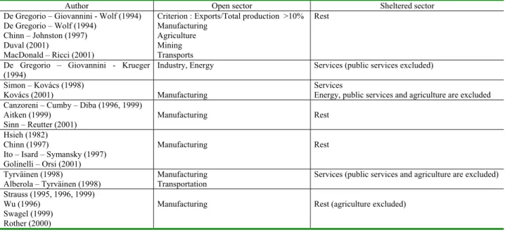
One crucial issue which arises when constructing productivity and relative price variables is how to define the tradable and the non-tradable sectors. No consensus has been reached in the literature on this issue (see Table 1 below). One of the most important issues seems to be the classification of agriculture. Owing to this and the limited availability on very detailed quarterly national accounts data, the process of defining the open and sheltered sectors mainly consisted of classifying agriculture. On the one hand, agricultural prices are not fully market-determined in the countries included in the sample. But on the other hand, the share of agricultural products in total exports is still rather high in a number of transition countries. We therefore constructed two types of productivity measures. First, agriculture and industry (excluding construction) are used to represent the tradable sector, while the rest is labelled non-tradable (Prod_A). Second, agriculture is dropped: the open sector now only consists of industry, whereas the sheltered sector covers everything else (Prod_B). If the level of and the change in productivity in agriculture is significantly different when compared with those in industry, the productivity differential between the traded and the non-traded goods sector - calculated according to these two measures - will differ. Average labour productivity is computed using the above classification as a base and by dividing the sectoral value added by the corresponding number of employees.
Table 1. An overview of sector classification
Author Open sector Sheltered sector
De Gregorio – Giovannini - Wolf (1994) De Gregorio – Wolf (1994)
Chinn – Johnston (1997) Duval (2001)
MacDonald – Ricci (2001)
Criterion : Exports/Total production >10% Manufacturing
Agriculture Mining Transports
Rest
De Gregorio – Giovannini - Krueger (1994)
Industry, Energy Services (public services excluded) Simon – Kovács (1998)
Kovács (2001) Manufacturing
Services
Energy, public services and agriculture are excluded Canzoreni – Cumby – Diba (1996, 1999)
Aitken (1999) Sinn – Reutter (2001)
Manufacturing Rest
Hsieh (1982) Chinn (1997)
Ito – Isard – Symansky (1997) Golinelli – Orsi (2001) Manufacturing Rest Tyrväinen (1998) Alberola – Tyrväinen (1998) Manufacturing Transportation
Services (public services and agriculture are excluded) Strauss (1995, 1996, 1999)
Wu (1996) Swagel (1999) Rother (2000)
Manufacturing Rest (agriculture excluded)
To measure the relative price of non-tradables, we first defined the relative price as being the ratio of the corresponding sectoral GDP deflators. The prices of non-tradables are given by the deflator for services obtained from the national accounts, and the deflator for tradables either given by the deflators for agriculture and industry (Defl_A), or just by the deflator for industry (Defl_B).
However, GDP deflators do not necessarily correspond to the officially published inflation indexes. Inflation is normally evaluated by looking at CPI and PPI rather than by using the corresponding sectoral deflators. The real exchange rate is also usually calculated using the CPI and PPI instead of GDP deflators. This is the main reason why we proceed to construct three measures for the relative price of non-tradables in terms of CPI and PPI. Data on price indices are mainly taken from the OECD (main economic indicators). Data from the IMF (IFS database) were however used when necessary series were not available from the OECD3.
1) First, we calculated the CPI / PPI (SERV1) ratio, which is often used as a proxy for relative prices. It assumes that all non-goods items in the CPI (which are expected not to be mirrored in PPI developments) are non-tradables. Therefore, this measure roughly corresponds to the ratio (non-tradables+tradables)/tradables. In practice, however, it has a number of drawbacks. The first issue to be dealt with is whether such a definition of tradables and non-tradables correctly reflects the relative price of non-tradables as the consumer price index can be roughly divided into food, durable goods, services, and regulated prices. It is worth being stressed that the regulated prices still have a substantial share in the consumer baskets of the transition countries (cf. Table 2.). And although services have the largest weight in the regulated prices, some items belong to the other two categories. Therefore, as all items other then industrial goods are considered as non-tradables, changes in e.g. food and regulated prices may cause some undesirable noise in the relative price measure. Furthermore, due to the relatively low income level, the share of services (including regulated prices) in CPI currently account for roughly 30% in most transition countries (see Table 3.). As a result, an increase in the productivity differential should increase the price differential – defined as CPI/PPI - only by a fraction of the productivity increase, and this fraction is given by the weight of services in the CPI. The problem is aggravated by the fact that regulated prices mainly concern services. Thus, the share of market driven service prices diminish in the CPI and attenuates the impact of productivity increases. Second, durable goods in the CPI are expected to correspond to the goods (usually industrial goods) included in the producer price index, which might be a heroic assumption. Hence, different movements in durable and industrial goods may affect the ratio.
3 We would like to note that series from these two databases are slightly different. Differences of several percentage
points can be observed in the CPI series obtained from the OECD and the IMF for Slovenia and Estonia. The same applies for the PPI series for Bulgaria, Hungary and Lithuania. However, the OECD series was used when available, and the IMF series only when OECD data were missing.
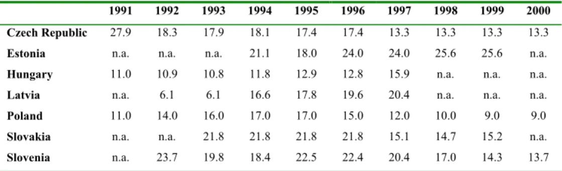
Table 2. The share of administered prices in the CPI basket, 1991-1999 (in %)
1991 1992 1993 1994 1995 1996 1997 1998 1999 2000 Czech Republic 27.9 18.3 17.9 18.1 17.4 17.4 13.3 13.3 13.3 13.3
Estonia n.a. n.a. n.a. 21.1 18.0 24.0 24.0 25.6 25.6 n.a.
Hungary 11.0 10.9 10.8 11.8 12.9 12.8 15.9 n.a. n.a. n.a.
Latvia n.a. 6.1 6.1 16.6 17.8 19.6 20.4 n.a. n.a. n.a.
Poland 11.0 14.0 16.0 17.0 17.0 15.0 12.0 10.0 9.0 9.0
Slovakia n.a. n.a. 21.8 21.8 21.8 21.8 15.1 14.7 15.2 n.a.
Slovenia n.a. 23.7 19.8 18.4 22.5 22.4 20.4 17.0 14.3 13.7 Source: EBRD, Transition Report 2001. Data for Croatia and Lithuania are not available from this source. It should be noted that data in Table 2 exclude some items treated as regulated elsewhere. Thus, data as in the Regular Reports by the European Commission coming from national sources are considerably higher than in Table 2. According to the 2001 Regular Reports, the share of regulated prices in CPI is as follows: 20.6% for Bulgaria , 18% for the Czech Republic, 15% for Estonia, 18.5% in Hungary, 22% for Latvia, 20.5% for Lithuania, 18% for Romania and 12.7% for Slovenia. According to national central bank reports, the share of regulated prices in the consumer price index is as high as 20.8% in Croatia (2002), 25.7% in Poland (2001) and 21.1% in Slovakia (2002).
Table 3. The share of services in the consumer price baskets (in %)
Food Industrial goods Services Year Source
Germany 13.1 24.24 62.7 1999 Federal Statstical Office
Croatia 19.5 56.8 21.4 2001 National Bank of Croatia Czech Republic 19.7 35.25 45.1
2002 Czech National Bank6
Estonia n.a. n.a. n.a. n.a.
Hungary 24.4 47.5 28.0 2002 Central Statistical Office, Hungary
Latvia n.a. n.a. n.a. n.a.
Lithuania n.a. n.a. n.a. n.a.
Poland 30.5 37.6 31.9 2000 National Bank of Poland Slovakia 27.6 32.4 39.7 2002 Statistical Office of the Slovak Republic Slovenia 22.0 49.0 29.0 2001 National Bank of Slovenia Notes: The category “food” does not contain the item “tobacco and alcoholic beverages” in most of the countries. Industrial goods include energy in most cases. In all countries except the Czech Republic, all categories comprise regulated prices. The classification into food, industrial goods and services was made by the indicated source. Only in the case of Germany is the classification based on the authors’ own calculations, assuming that the COICOP categories no. 2,3,5 and 12 are tradable goods.
2) Second, the ratio of services in CPI to the CPI (SERV2) is considered. This ratio corrects some of the shortcomings of the CPI/PPI ratio as the noise from service prices is eliminated and the possibly low comparability in durable and industrial goods is lifted. In fact, the ratio can be viewed as non–tradable prices over (tradable + non-tradable prices). It must however be noted that the inclusion of regulated items in the service category remains a problem. The OECD does not offer series on services explicitly excluding regulated prices for all countries. Therefore it may be the case that for some countries, the category “CPI services“ includes the regulated prices, and for others not – with according consequences for the test results. Moreover, the noise in service prices brought about by the
4 Non-food tradables
5 Non-food tradables
6 The classification into tradables and non-tradables is taken from the Quarterly Reports on Inflation of the Czech
National Bank (CNB). The CNB is not calculating the consumer price index, so that this classification mainly reflects the CNB’s assessment of the tradability of these items. In 2002, the CNB proceeded to considerably reclassify these items. This was not accompanied by the necessary adjustments needed in the consumer basket published by the Statistical Office. Until 2001, the weights were as follows: 32.7% for food (incl. tobacco), 34.6% for tradables and 32.7% for non-tradables.
inclusion of miscellaneous categories in services is shifted towards tradable prices since all categories but service prices are defined as being tradable.
3) The third, and obviously the best ratio for measuring relative prices is services in CPI over PPI (SERV3). This measure will be close to the definition using deflators, because the two chosen components in the CPI most reflect closely the deflator measures. A drawback of this measure is however, that from this measure it cannot be inferred what impact the increase in the service prices has on overall inflation.
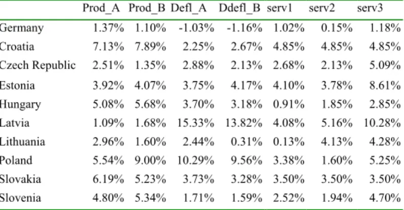
Table 4. An overview of data, yearly averages, 1995-2000
Prod_A Prod_B Defl_A Ddefl_B serv1 serv2 serv3 Germany 1.37% 1.10% -1.03% -1.16% 1.02% 0.15% 1.18% Croatia 7.13% 7.89% 2.25% 2.67% 4.85% 4.85% 4.85% Czech Republic 2.51% 1.35% 2.88% 2.13% 2.68% 2.13% 5.09% Estonia 3.92% 4.07% 3.75% 4.17% 4.10% 3.78% 8.61% Hungary 5.08% 5.68% 3.70% 3.18% 0.91% 1.85% 2.85% Latvia 1.09% 1.68% 15.33% 13.82% 4.08% 5.16% 10.28% Lithuania 2.96% 1.60% 2.44% 0.31% 0.13% 4.13% 4.28% Poland 5.54% 9.00% 10.29% 9.56% 3.38% 1.60% 5.25% Slovakia 6.19% 5.23% 3.73% 3.28% 3.50% 3.50% 3.50% Slovenia 4.80% 5.34% 1.71% 1.59% 2.52% 1.94% 4.70%
The real exchange rate is calculated using the CPI. Nominal exchange rates are measured in foreign currency terms and are averages of average monthly data. Nominal exchange rates are extracted from the WIIW monthly database for transition economies.
5. Estimation techniques
The use of quarterly data and the short sample period makes the use of time series techniques extremely difficult. We therefore employ panel techniques, namely recent panel unit root and panel cointegration tests. First, the order of integration of the time series has to be investigated. For this purpose, the Im-Pesaran-Shin (1997) (IPS) panel unit root test is used. The IPS test is based on individual ADF statistics. The t-bar statistic constructed as a mean of individual ADF statistics is used to test the null hypothesis of a unit root. This test is used instead of the usual Levin and Lin test, because it allows for a high degree of heterogeneity across the countries of the panel, e.g. in the autoregressive coefficient and the lag used for each country. When investigating the presence of a unit root in the series, a model assuming a trend and an intercept and, a model containing only a constant are tested for.
(15)
∆
y
π
y
n 1b
∆
y
i,t 1 i it
i,t,
i
1
,
2
,...,
N
;
t
1
,
2
,...,
T
1 t i 1 t i, t i,=
⋅
+
⋅
−+
+
⋅
+
=
=
− = −∑
µ
γ
ε
,(16)
∆
y
π
y
n 1b
∆
y
i,t 1 i i,t,
i
1
,
2
,...,
N
;
t
1
,
2
,...,
T
1 t i 1 t i, t i,=
⋅
+
⋅
−+
+
=
=
− = −∑
µ
ε
The null of H0 :πi =0 for each i is tested against the alternative hypothesis of
N ,..., 1 N i, 0 , N ,..., 2 , 1 i, 0 :
H1 πi < = 1 πi = = i + . If the presence of a unit root is rejected in Equation (15), we cannot exclude the possibility that the series are stationary around a trend as we do not have information on whether or not the trend is statistically significant. For this reason, we also have to test for equation (16). A major inconvenience while testing for equation (5) is that some series of the panel might contain a deterministic trend while others can have a stochastic trend. Unfortunately, the IPS test is not able to allow for heterogeneity in the trend.
Reported in Tables 1-2 of Appendix, results of the IPS tests for the investigated series show that the IPS test including a trend reject the presence of a unit root around a linear trend. However, test results are not always very robust against the number of lags used. As it is extremely difficult to decide whether the trend is significant and thus the series TS, we also employ equation (16) including only a constant: the hypothesis of a unit root cannot be never rejected, whatever lag is used. At the same time, in first differences, both equation (15) and (16) can clearly reject the presence of a unit root. So, we can conclude that the series are non-stationary processes.
The I(1) nature of the pooled series makes the use of cointegration tests necessary. Pedroni (1997) suggested seven tests statistics, which can be used for detecting long-run cointegration relationships. All tests use residuals of a Engle-Granger-type cointegration regression as shown below:
T ,..., 2 , 1 t ; N ,..., 2 , 1 i, t x yi,t =αi +βi⋅ i,t +δi⋅ +εit, = = . (17)
The null of no cointegration against the alternative hypothesis of cointegration is tested for using the residuals extracted from equation (17). The null hypothesis for the panel cointegration tests is that the investigated series are not cointegrated. Of the proposed seven tests statistics, four test statistics (panel v-statistic, panel rho-v-statistic, panel pp-v-statistic, panel ADF-statistic) are based on pooling along the within-dimension. The null hypothesis is H0: π =1 (i.e. no cointegration) for all cross-sectional units versus the alternative hypothesis H1: πi = π<1 for all cross-sectional units so that a common slope value of lag one residuals is presumed in the residual test equations. By contrast, the other three test statistics (group rho-statistic, group pp-rho-statistic, group ADF-statistic) are based on pooling along the between-dimension. The alternative hypothesis is H1: πi <1 for all i so that it allows for different values of the autoregressive term. Pedroni (1997) showed that for values of T larger than 100, the proposed seven statistics do equally well and are quite stable. However for smaller samples (T inferior to 20), the Group ADF-statistic is the most
powerful among the group statistics. For this reason, only this latter test statistic will be reported. The coefficients of the cointegrating vector are then determined using the panel fully modified ordinary least squares (FMOLS) estimator by Pedroni (2000). The lag length is allowed to differ across countries and is determined using the Newey-West method. As for the unit root tests, we face the problem of heterogeneous trends: in the cointegration relationship, some countries might have a trend whereas other might not have. Another important drawback when using panel techniques is that it is not possible to conclude on the robustness of the relationship and the size of the estimated coefficient for individual countries. In contrast, what we can say is that a given cointegration relationship is verified on average for a set of countries. This also applies for the estimated coefficient reflect some sort of mean of heterogeneous individual coefficients. We therefore will reason in terms of a group of countries when interpreting empirical results, and will focus more on the comparison of the determined values than on the precise number.
6. Results
6.1 Investigating the basic assumptions of the model
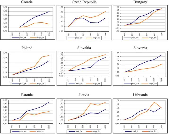
Before testing for the internal relationship between relative productivity and relative prices, two crucial hypothesis have to be analysed: Whether or not real wages in the tradable sector are connected to productivity growth and whether wage increases tend to equalise between the open and sheltered sectors. Figures 1 and 2 show that in most countries, the assumptions seem to be fulfilled. On the one hand, using industry for the traded goods sector, real wages in the traded goods sector deflated by the corresponding sectoral deflator move broadly in line with productivity growth. On the other hand, we can observe that nominal wages develop similarly in the open and sheltered sector with the exception of Croatia. However, there are notable differences between countries: While productivity increases outpace real wage increases in Croatia, Estonia, Hungary and Slovenia, the opposite is found in the other countries.
Figure 1. Productivity and real wage developments in industry
Note: Productivity is average labour productivity in industry while real wage is the nominal wage in industry deflated by the sectoral deflator 0,90 0,95 1,00 1,05 1,10 1,15 1,20 1,25 1,30 19 95 19 96 19 97 19 98 19 99 20 00 prod_hu wage_hu 0,90 1,10 1,30 1,50 1,70 1,90 19 95 19 96 19 97 19 98 19 99 20 00 prod_pl wage_pl 0,90 1,00 1,10 1,20 1,30 1,40 1,50 1995 1996 1997 1998 1999 2000 prod_cr wage_cr 0,90 1,00 1,10 1,20 1,30 1,40 1995 1996 1997 1998 1999 2000 prod_cz wage_cz 0,90 0,95 1,00 1,05 1,10 1,15 1,20 1,25 1,30 1,35 1995 1996 1997 1998 1999 2000 prod_sk wage_sk 0,90 1,00 1,10 1,20 1,30 1,40 1,50 19 95 19 96 19 97 19 98 19 99 20 00 prod_svn wage_svn 0,90 1,00 1,10 1,20 1,30 1,40 1,50 1,60 1 995 1996 1997 1998 1999 2000 prod_ee wage_ee 0,90 1,00 1,10 1,20 1,30 1,40 1,50 1,60 1995 1996 1997 1998 1999 2000 prod_lv wage_lv 0,90 1,00 1,10 1,20 1,30 1,40 1,50 19 95 19 96 19 97 19 98 19 99 20 00 prod_li wage_li
Croatia Czech Republic Hungary
Poland Slovakia Slovenia
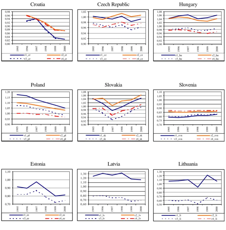
Figure 2. The nominal wage equalisation process across sectors
Note: r1 represents nominal wage in industry over nominal wage in non-tradable sectors whereas r2 is wage in industry over nominal wage in the whole economy. Nominal wage in the sheltered sector is average nominal wages in all sectors excepted industry and agriculture weighted with the number of employees in the corresponding sector. r3 and r4 are computed as average nominal wages in industry and agriculture over nominal wages in the rest and in the whole economy, respectively. Once again, the average of wages in industry and agriculture is calculated using the number of sectoral employees as weights.
0,80 0,82 0,84 0,86 0,88 0,90 0,92 0,94 0,96 0,98 1995 1996 1997 1998 1999 2000 r1_cr r2_cr r3_cr r4_cr 0,90 0,92 0,94 0,96 0,98 1,00 1,02 1995 1996 1997 1998 1999 2000 r1_cz r2_cz r3_cz r4_cz 0,90 0,92 0,94 0,96 0,98 1,00 1,02 1,04 1,06 1,08 1995 1996 1997 1998 1999 2000 r1_hu r2_hu r3_hu r4_hu 0,90 0,95 1,00 1,05 1,10 1,15 1,20 1995 1996 1997 1998 1999 2000 r1_pl r2_pl r3_pl r4_pl 0,90 0,92 0,94 0,96 0,98 1,00 1,02 1,04 1,06 1,08 1995 1996 1997 1998 1999 2000 r1_sk r2_sk r3_sk r4_sk 0,70 0,75 0,80 0,85 0,90 0,95 1,00 1,05 1,10 1995 1996 1997 1998 1999 2000 r1_svn r2_svn r3_svn r4_svn 0,50 0,60 0,70 0,80 0,90 1,00 1,10 1,20 1,30 1995 1996 1997 1998 1999 2000 r1_li r2_li r3_li r4_li 0,70 0,80 0,90 1,00 1,10 1995 1996 1997 1998 1999 2000 r1_ee r2_ee r3_ee r4_ee 0,60 0,70 0,80 0,90 1,00 1,10 1,20 1,30 1995 1996 1997 1998 1999 2000 r1_lv r2_lv r3_lv r4_lv
Croatia Czech Republic Hungary
Poland Slovakia Slovenia
6.2 The internal transmission mechanism from productivity growth towards non-tradable inflation
As shown in Table 5., the group ADF test can detect the presence of a correctly signed, statistically significant cointegration relationship between productivity and relative prices based on the corresponding deflator series. The result is robust with regard to the inclusion of a trend. The size of the estimated coefficient changes considerably upon whether or not agriculture is included in the open sector. The coefficient of 1.00 obtained including agriculture in the open sector (Prod_A–Defl_A) suggests that increases (decreases) in productivity are connected with corresponding increases (decreases) in the relative price of non-tradables. Excluding agriculture leads to a coefficient of only 0.73 (Prod_B-Defl_B), indicating that a rise (fall) in productivity exceeds the rise (fall) in relative prices. The higher coefficient obtained for Prod_A-Defl_A (1.00) compared to that for Prod_B - Defl_B (0.73) may be due to the fact that, on average, productivity gains in industry by far outpaced those in agriculture. At the same time, the relative price of non-tradables seems to be less sensitive to whether or not agricultural prices are included. Put differently, prices in agriculture developed similarly with other tradable prices. The finding that the two coefficients significantly differ implies that the assessment of the Balassa-Samuelson effect is sensitive to the classification employed.7
When the three price index-based relative price measures (serv1, serv2, serv3) are used instead of relative prices computed using GDP deflators (Defl_A, Defl_B), it is much more difficult to detect robust cointegrating vectors between productivity and relative prices. As shown in Table 5., results seem to be very fragile for the inclusion of a trend. The tests cannot establish virtually any cointegration relationship. In fact, cointegration is only found for the ratio serv2 (i.e. the ratio of service prices in the CPI to headline CPI) including a trend. In general, we can observe that the few estimated coefficients are considerably lower compared to those obtained using GDP deflators. One reason for this may be the fact that tradable prices in CPI grew faster than those included in the sectoral deflators. Another important factor is the high share of goods with substantial price increases in the CPI, such as energy, which is still regulated in all transition countries concerned. This can easily reduce the impact of higher services inflation on the relative price ratio. Therefore, the estimated coefficients of 0.43 and 0.57 show that the development of the other components in the consumer price index will also be of importance when determining the path of the relative price of non-tradables. And this finding is even more compelling as services including regulated items should basically increase this ratio independently on productivity increases.
7 We note that all the estimations have also been carried out for a panel including Bulgaria and Romania. However,
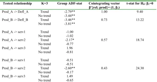
Table 5.
Panel cointegration tests for the internal transmission mechanism
Tested relationship K=3 Group ADF-stat Cointegrating vector
β'{rel; prod}= (1, β1)
t-stat for H0: β1=0
Prod_A -> Defl_A Trend -2.79** 1.00 9.40
No trend -3.44**
Prod_B -> Defl_B Trend -3.46** 0.73 13.22
No trend -3.81**
Prod_A -> serv1 Trend -1.00
No trend -1.02
Prod_A -> serv2 Trend -2.17* 0.57 18.74
No trend -0.77
Prod_A -> serv3 Trend 1.96
No trend -0.81
Prod_B -> serv1 Trend -0.51
No trend -0.51
Prod_B -> serv2 Trend -2.60** 0.43 24.30
No trend -0.17
Prod_B -> serv3 Trend 1.49
No trend -0.65
Notes: ** and * denote that results are significant at the 1% and 5% level, respectively.
6.3 The external transmission mechanism
When it comes to investigating the external relationship explaining inflation differentials and real exchange rate developments, a reference country is to be chosen. In this study, Germany serves as the benchmark country since it is the most important trade partner of the countries included in the panel (cf. Eurostat 2001b).
In accordance with equation (11), we proceed to analyse the external relationship. Results of the cointegration analysis (see Table 6.) are very similar to those obtained for the internal transmission mechanism. The panel cointegration tests are able to reject the null of no cointegration indicating the presence of a cointegrating vector connecting the productivity differential and the sectoral deflator-based relative price differential vis-à-vis Germany. Furthermore, the estimated coefficients are statistically significant and correctly signed except one coefficient. Similarly to what we found earlier, the coefficient estimated using agriculture as part of the open sector (1.11) is higher than when agriculture is excluded from the analysis (0.89). We note, however, that the former is not statistically significant. For these differing coefficients, an explanation is provided by the fact that the exclusion of agriculture increases the productivity differential in CEECs and reduces it in Germany, without correspondingly affecting relative prices8. The positive coefficient of less than 1 would imply that if changes in relative prices and the
8 We note that Germany experienced substantial productivity increases in agriculture. This does not significantly
distort tradable and non-tradable productivity measures, as agriculture has only a low weight in German GDP. But, more importantly, productivity gains higher in industry than in the service sector were accompanied by declining sectoral deflator-based relative prices. This development is however not reflected in the price indices. The CPI/PPI ratio (serv1) and CPI services over PPI (serv3) show a slight upward movement, while CPI services and CPI series move together as services account for 70% in German CPI. Consequently, CPI services over CPI (serv2) is very
sectoral productivity differential in the home country outpace those in Germany, changes in the productivity differential vis-à-vis Germany lead to less than proportionate increases in the sectoral deflator-based relative price of non-tradable goods.
Similarly to what is found for the internal transmission mechanism, the panel cointegration tests are not able to accept the presence of cointegration between productivity and price-index-based relative prices (serv1, serv2, serv3). The only measure for which we find a long-term relationship, is the CPI serv/CPI ratio. Again, the estimated coefficients are lower compared to those obtained using deflator based relative prices. This is an important finding. Basically, the serv2 measure is the least suited for assessing the real appreciation of the currency associated with the Balassa Samuelson effect, because the majority of items in the consumer baskets are services in Germany. As a result, the serv2 measure is rather stable implying that the differential of serv2 of the home country and Germany are expected to be sizeable. This lends further evidence to the problem already mentioned regarding the developments of other components in the transition countries’ consumer basket.
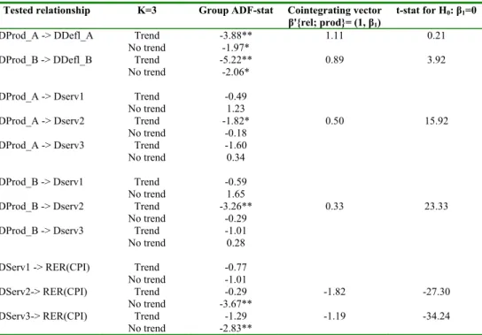
Table 6.
Panel cointegration tests for the external transmission mechanism
Tested relationship K=3 Group ADF-stat Cointegrating vector
β'{rel; prod}= (1, β1)
t-stat for H0: β1=0
DProd_A -> DDefl_A Trend -3.88** 1.11 0.21
No trend -1.97*
DProd_B -> DDefl_B Trend -5.22** 0.89 3.92
No trend -2.06*
DProd_A -> Dserv1 Trend -0.49
No trend 1.23
DProd_A -> Dserv2 Trend -1.82* 0.50 15.92
No trend -0.18
DProd_A -> Dserv3 Trend -1.60
No trend 0.34
DProd_B -> Dserv1 Trend -0.59
No trend 1.65
DProd_B -> Dserv2 Trend -3.26** 0.33 23.33
No trend -0.29
DProd_B -> Dserv3 Trend -1.01
No trend 0.28
DServ1 -> RER(CPI) Trend -0.77
No trend -1.01
DServ2-> RER(CPI) Trend -0.29 -1.82 -27.30
No trend -3.67**
DServ3-> RER(CPI) Trend -1.29 -1.19 -34.24
No trend -2.83**
Notes: ** and * denote that results are significant at the 1% and 5% level, respectively. “Dserv” and “Dprod” indicate the difference between the countries considered and Germany.
Testing the relationship as in equation (14) allows us to check whether the CPI-deflated real exchange rate and the relative prices based on price indexes are cointegrated, to what extent the real appreciation can be
explained by the Balassa-Samuelson effect, i.e. whether the actual real appreciation corresponds to what the tests carried out on relative productivity and price developments suggest. For this exercise, we use the following, slightly modified version of equation (14):
(14’)
=
*
P
*
P
P
P
1
Q
t nt t ntAs can been seen in Table 6., the group ADF test can accept the presence of statistically significant and well signed cointegrating vectors between the CPI-based real exchange rate and the difference of the relative price of non-tradables when Dserv2 and Dserv3 are used. However, the estimated coefficients show that the observed real appreciation has been higher than what the Balassa-Samuelson effect would suggest. According to equation (14), the coefficient should correspond to the share of non-tradables in the consumer price basket. If these weights differ in the home and foreign countries and they are stable over time, the estimated value should be somewhere between the two weights. By contrast, the estimated coefficients shown in Table 6 exceed unity.
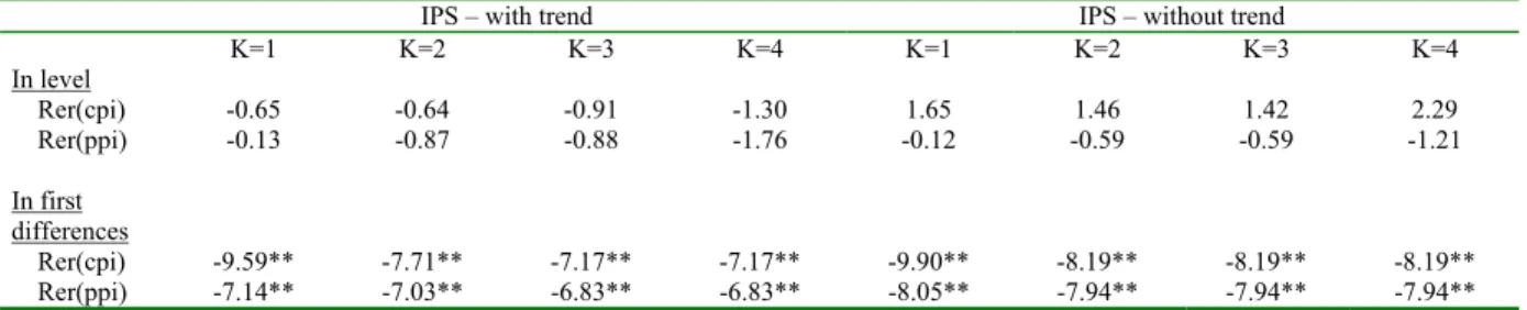
As a matter of fact, the test is based on the assumptions that PPP holds for tradables. However, PPP does not seem to be verified for the traded goods sector. Visual inspection of Figure 3. clearly shows that the PPI-deflated real exchange rate appreciates in most of the countries as does the CPI-deflated real exchange rate. The only difference visible to the naked eye is the slightly smaller extent of the appreciation of the PPI-deflated real exchange rate. The IPS panel unit root tests provide further evidence against PPP in the open sector. According to the results reported in Table 7., the hypothesis of a unit root cannot be rejected in levels. This shows that the PPI-deflated real exchange rates are not stationary. Another piece of evidence is provided in Table 8, which shows the results of cointegration tests carried out between the PPI-deflated real exchange rate and the three price index-based relative prices measures (Dserv1, Dserv2, Dserv3). The results are very close to those performed for the CPI-based real exchange rate and relative prices. Contrary to what we expect, the PPI-based real exchange rate is found to be cointegrated with Dserv2 and Dserv3, when no trend is included in the cointegrating vector. As suggested by Figure 3., the estimated coefficients are lower than those found for the CPI-based real exchange rate. These results suggest that the increase in the relative price of non-tradables is accompanied by a trend increase in traded
Table 7. IPS panel unit root tests for the CPI and PPI-based real exchange rates
IPS – with trend IPS – without trend
K=1 K=2 K=3 K=4 K=1 K=2 K=3 K=4 In level Rer(cpi) -0.65 -0.64 -0.91 -1.30 1.65 1.46 1.42 2.29 Rer(ppi) -0.13 -0.87 -0.88 -1.76 -0.12 -0.59 -0.59 -1.21 In first differences Rer(cpi) -9.59** -7.71** -7.17** -7.17** -9.90** -8.19** -8.19** -8.19** Rer(ppi) -7.14** -7.03** -6.83** -6.83** -8.05** -7.94** -7.94** -7.94** Note: Critical values are those for the one-sided normal distribution.
Table 8.
Panel cointegration tests for the PPI-based real exchange rate and relative prices
Tested relationship K=3 Group ADF-stat Cointegrating vector
β'{rel; prod}= (1, β1)
t-stat for H0: β1=0
DServ1 -> RER(PPI) Trend -0.31
No trend -0.83
DServ2-> RER(PPI) Trend -0.79 -1.30 -23.21
No trend -3.53**
DServ3-> RER(PPI) Trend -0.13 -0.70 -25.03
No trend -2.32*
Notes: ** and * denote that results are significant at the 1% and 5% level, respectively.
Hence, the role of the productivity driven non-tradable inflation might be of limited importance as to the appreciation of the CPI-deflated real exchange rate. In view of the real appreciation that the countries in the panel have experienced, other factors seem to be more important for the real appreciation. An obvious candidate are producer prices. As can be seen in Figure 3, the appreciation of the PPI-based real exchange rates has been sizeable in most countries. What’s more, this tradable based real appreciation differs only slightly from the CPI-based real appreciation in some countries. This, however, is less surprising when recalling the small weight of the non-tradables in the consumer basket (see Table 3.). This is indeed in line with Ito et al. (1997). Analysing fast growing East Asian economies, they come to the conclusion that in some of these countries productivity advances are connected with higher tradable price inflation compared to the outside world and thus a real appreciation of the producer price deflated exchange rate.
Figure 3. The CPI and the PPI deflated real exchange rate vis-à-vis Germany
The real appreciation of the PPI-deflated real exchange rate is somewhat puzzling in light of the Balassa-Samuelson model, which assumes that PPP holds for traded goods. In the transition economies studied here, lower real income is not only caused by lower productivity in the production of the same traded goods, but also because of a reduced ability to produce goods of higher technological content. This is exacerbated by smaller capital stocks and the lack of know-how as well as institutional factors hindering productivity such as poor corporate governance, weak public administration, insufficient legislation and low-quality infrastructure. At the beginning of the 1990s, the transition countries mainly exported food, manufactured goods and machinery of a lower quality and technological content. The driving force behind the Law of One Price and PPP is the goods arbitrage process, which ensures that the price of the same good, expressed in the same currency, is the same at home and abroad through adjustments in the nominal
-0,18 -0,16 -0,14 -0,12 -0,10 -0,08 -0,06 -0,04 -0,020,00 0,02 0,04 19 95:Q 1 19 95:Q 4 19 96:Q 3 19 97:Q 2 19 98:Q 1 19 98:Q 4 19 99:Q 3 20 00:Q 2 20 01:Q 1 20 01:Q 4 cr_rer_cpi cr_rer_ppi -0,45 -0,40 -0,35 -0,30 -0,25 -0,20 -0,15 -0,10 -0,050,00 0,05 1995:Q1 1995:Q4 1996:Q3 1997:Q2 1998:Q1 1998:Q4 1999:Q3 2000:Q2 2001:Q1 2001:Q4 cz_rer_cpi cz_rer_ppi -0,35 -0,30 -0,25 -0,20 -0,15 -0,10 -0,05 0,00 0,05 0,10 1995:Q1 1995:Q4 1996:Q3 1997:Q2 1998:Q1 1998:Q4 1999:Q3 2000:Q2 2001:Q1 2001:Q4 hu_rer_cpi hu_rer_ppi -0,60 -0,50 -0,40 -0,30 -0,20 -0,10 0,00 0,10 19 95:Q1 19 95:Q4 19 96:Q3 19 97:Q2 19 98:Q1 19 98:Q4 19 99:Q3 20 00:Q2 20 01:Q1 20 01:Q4 pl_rer_cpi pl_rer_ppi -0,35 -0,30 -0,25 -0,20 -0,15 -0,10 -0,05 0,00 0,05 19 95: Q1 19 95: Q4 19 96: Q3 19 97: Q2 19 98: Q1 19 98: Q4 19 99: Q3 20 00: Q2 20 01: Q1 20 01: Q4 sk_rer_cpi sk_rer_ppi -0,12 -0,10 -0,08 -0,06 -0,04 -0,02 0,00 0,02 0,04 1995: Q 1 1995: Q 4 1996: Q 3 1997: Q 2 1998: Q 1 1998: Q 4 1999: Q 3 2000: Q 2 2001: Q 1 2001: Q 4 svn_rer_cpi svn_rer_ppi -0,60 -0,50 -0,40 -0,30 -0,20 -0,10 0,00 1995: Q 1 1995: Q 4 1996: Q 3 1997: Q 2 1998: Q 1 1998: Q 4 1999: Q 3 2000: Q 2 2001: Q 1 2001: Q 4 ee_rer_cpi ee_rer_ppi -0,70 -0,60 -0,50 -0,40 -0,30 -0,20 -0,10 0,00 19 95 :Q 1 19 95 :Q 4 19 96 :Q 3 19 97 :Q 2 19 98 :Q 1 19 98 :Q 4 19 99 :Q 3 20 00 :Q 2 20 01 :Q 1 20 01 :Q 4 lv_rer_cpi lv_rer_ppi -0,90 -0,80 -0,70 -0,60 -0,50 -0,40 -0,30 -0,20 -0,100,00 0,10 0,20 199 5: Q 1 199 5: Q 4 199 6: Q 3 199 7: Q 2 199 8: Q 1 199 8: Q 4 199 9: Q 3 200 0: Q 2 200 1: Q 1 200 1: Q 4 li_rer_cpi li_rer_ppi
Croatia Czech Republic Hungary
Poland Slovakia Slovenia
exchange rate and prices. Even though trade barriers have been quickly abolished between the EU and the transition countries, due to the mismatch of exports and imports and the lack of suitable counterparts, the exchange rate is most probably determined not by good arbitrage, but rather by balance of payments developments. Although exports have shifted to more technology intensive goods, this has not prevented some transition countries from remaining highly specialised (Eurostat 2001c).
During the transition process, export and supply capacities of the countries concerned have significantly increased owing to the increasing technological content and quality of products. This is well recognised in studies analysing the structure of foreign trade (Cf. Havlik et al.(2001), for all transition countries and Darvas-Sass (2002) for Hungary). In fact, part of the higher productivity in the tradable sector reflects this ability to produce goods of higher quality and thus to sell them at higher prices. If this quality improvement is not adequately accounted for when calculating inflation9, higher quality will be translated into an increase in producer prices. Furthermore, as all tradable goods have a non-tradable component, the productivity driven catch-up of non-tradable prices will automatically be reflected in traded goods prices. This is a hidden transmission mechanism between productivity and prices, which cannot be seen in official statistics. If the appreciation of the PPI-based real exchange rate does indeed reflect the increased ability to produce goods in higher price and quality segments, this would imply that a part of the price level convergence results from the shift to new goods (goods of higher quality and prices), i.e. without inflation (cf. Ferenczi et al (2000), Lommatzsch/Tober (2002)).
Figure 3. shows that the size of the CPI and PPI-based real appreciation that the individual countries in the study have experienced differs substantially. According to popular belief, the magnitude of the observed real appreciation is closely related to the exchange rate regime. In addition, also the real appreciation linked to the Balassa-Samuelson effect may be connected to the exchange rate regime. We think, however, that it is rather unlikely that the exchange rate regime could affect the productivity driven real appreciation, because the Balassa-Samuelson model describes a microeconomic equilibrium process independent of the exchange rate regime. If PPP holds for traded goods, the relative price of non-traded goods, given by the production functions, determines the real exchange rate. In general a change in the real exchange rate may occur either through changes in prices or via movements in the nominal exchange rate. However, according to the Balassa-Samuelson model, real appreciation of the currency can only occur through a nominal appreciation if the adjustment in relative prices requires more liquidity, which is not added to the economy, so that tradables prices decline and nominal appreciation follows. In contrast, in
9 According to the SDDS of the IMF, not all statistical offices in the investigated countries adjust their PPI measures
most transition countries adjustments in the relative price of non-tradables took place through an upward movement in nominal prices. Furthermore, the downward adjustment of the nominal price of tradables – if it occurred at all – followed an appreciation of the nominal exchange rate. Therefore, the nominal appreciation of the currency that occurred in some transition economies and thus any real appreciation that is not linked to productivity advances have other sources. It is not the exchange rate regime as such, but the circumstances surrounding it that affect the real appreciation of a currency and movements in the exchange rate. The most important of these factors is the extent of currency convertibility, i.e. the amount of permitted current and capital account transactions, the ability and willingness of central banks to sterilise capital inflows, and the use of the exchange rate for macroeconomic stabilisation or trade balance developments (targeting a real exchange rate). Fixed exchange rates are usually connected with restrictions on or sterilisation of capital flows, restrictions on capital flows are most often needed to allow the central bank to target the development of the real exchange rate. The transition countries have opted for capital controls to differing extents (Corker et al. (2000)). Such differences affected the nominal exchange rate or the price level, especially in those transition countries that have been subject to a constant flow of inward investments for a number of years.
7. Conclusions
Using the Pedroni panel cointegration technique, we showed that the productivity growth differential between the open and the sheltered sectors are strongly linked to increases in the relative price of non-tradables when using detailed national account data for productivity and relative prices. Moreover, whether agriculture is classified as part of the open sector may considerably modify results since on average, productivity and price developments do substantially differ in that sector. As a consequence, it may be better not to consider agriculture as a traded good sector. When the relationship between the productivity differential between tradables and non-tradables and different measures for relative prices calculated using price indexes such as CPI and PPI is considered, we found it extremely difficult to detect robust cointegrating vectors. This is not surprising given the structure of the consumer price index. First, the share of non-tradables in CPI is very low, close to 30% on average in the countries considered. Furthermore, regulated prices still account for between 15% and 25% of the consumer price index, which is also likely to bias price development for several reasons. First, increases in administered prices can exceed rises in non-tradable inflation. Second, changes in administered prices can be erratic depending on politically motivated decisions. As long as goods with regulated prices are important input factors (energy, transport), their adjustments may constitute another cost push factor for non-tradables prices. These results therefore suggest that the role of the Balassa-Samuelson effect in the price level convergence (and the real appreciation of the currency) might be limited. and that other factors may be of greater importance. One
major consequence of the mismatch between the non-tradables’ share within the GDP (around 60-70%) and the consumer price basket (20-30%) is the following: When measuring price level in terms of the GDP deflator and inflation in terms of CPI, it is true to say that price level convergence through increases in productivity driven non-tradable prices can be achieved without correspondingly high inflation.
The occurrence of the Balassa Samuelson effect in the transition countries is often seen in connection with their adoption of the euro and the preparations for it in line with the Maastricht criteria. For instance, Halpern and Wyplosz (2001) and Szapáry (1999) argue that the sizeable catch-up in the traded goods sector’s productivity will lead to higher inflation, which could make it impossible to achieve either the inflation criterion of a maximum of 1,5% higher than the three EMU member countries with the lowest inflation rate, or the exchange rate criterion, i.e. that the exchange rate should be fixed for two years within the ERM II using bands of +/-15% around the central parity. Likewise, Buiter and Grafe (2002) maintain that it could be that only the countries that apply these large bands may manage to fulfil the criteria, using the band for constant nominal appreciation and thus manage to keep overall inflation within the required limits.
For the sake of illustration, we computed average yearly values for the productivity differential between open and sheltered sectors for every country considered. We then used the share of services in CPI as in Table 3 so as to determine the scale of the productivity driven service inflation on overall inflation. In this exercise, we assume than 1% change in productivity bring about 1% change in service prices. Results presented in Table 9 clearly show that even in the case of high productivity growth countries such as Poland, the inflation brought about productivity growth of 2.87% is just a fraction of the initial productivity differential of 9%. The composition of the consumer baskets and especially the share of non-tradables is of importance when determining the role productivity induced non-tradable price increases play in overall inflation. As long as the weight of non-tradables remains low (in particular in comparison with that of the average consumer basket of EU-countries), the impact of the effect on overall inflation remains limited. By contrast, even though the growth rate of the productivity differential averages to a mere yearly 1.1%-1.37% in Germany, the inflation attributable to the Balassa-Samuelson effect is relatively high as shown in column 4 and 5 of Table 9.
As a result, the inflation differential vis-à-vis Germany based on productivity advances is indeed very low. Figures are either negative or very close to zero for the Czech Republic, Latvia and Lithuania, range from 0.3% to 0.5% for Estonia and are established between 0.5% and 1% for Croatia, Hungary and Slovenia. The inflation differential is as high as 1.6% and 2.18% for Slovakia and Poland when using Prod_A and Prod_B, respectively. This implies that if Germany is considered as a good benchmark for the Maastricht
criterion on inflation, these two countries might have encountered some difficulties on account of the Balassa-Samuelson effect. Nevertheless, these figures are, once again, very sensitive to whether agriculture is considered as a traded good sector since they drop below 1.5% when using a different classification. All this can mean that concerns as to the conflict between nominal and real convergence may be not that well-funded.
Table 9. Productivity growth, productivity growth driven service inflation and inflation differential
vis-à-vis Germany, 1995-2000
Prod_A Prod_B Share of services in CPI( G ) P(fProd_A) P(Prod_B) dP(Prod_A) dP(Prod_B)
Germany 1,37% 1,10% 62,7% 0,86% 0,69% 0,00% 0,00% Croatia 7,13% 7,89% 21,4% 1,53% 1,69% 0,67% 1,00% Czech Republic 2,51% 1,35% 32,7% 0,82% 0,44% -0,04% -0,25% Estonia 3,92% 4,07% 30,5% 1,19% 1,24% 0,34% 0,55% Hungary 5,08% 5,68% 28,0% 1,42% 1,59% 0,56% 0,90% Latvia 1,09% 1,68% 30,5% 0,33% 0,51% -0,53% -0,18% Lithuania 2,96% 1,60% 30,5% 0,90% 0,49% 0,04% -0,20% Poland 5,54% 9,00% 31,9% 1,77% 2,87% 0,91% 2,18% Slovakia 6,19% 5,23% 39,7% 2,46% 2,07% 1,60% 1,39% Slovenia 4,80% 5,34% 29,0% 1,39% 1,55% 0,53% 0,86%
Prod_A, Prod_B: average yearly growth rate of the productivity differential over 1995-2000
Share of services in CPI as in Table 3.. As data are not available for Estonia, Latvia and Lithuania, the average of the other transition countries is used for the Baltic States.
P(Prod_A), P(Prod_B): Prod_A and Prod_B multiplied by the share of services in CPI
dP(Prod_A): the difference between P(Prod_A) of the country considered and P(Prod_A) for Germany dP(Prod_B): the difference between P(Prod_B) of the country considered and P(Prod_B) for Germany
At the same time, these figures also stand for the real appreciation, which can be justified by the Balassa-Samuelson effect. They seem to be very small, especially in light of the observed real appreciation. In fact, there are other factors, which can lead to the real appreciation of the exchange rate, and which are also related to the catch-up process. The price level convergence of the transition economies is also taking place through an increase in the prices of tradables, which is reflected in PPI-based real exchange rate movements. Because at least a part of the increase in the tradables’ price level comes through a shift to goods of higher quality (and higher prices), this does not need to be reflected in the inflation measures. However, it can – depending on adjustments for quality changes and for the inclusion of new goods. Hence a basic problem of the transition countries is to determine to what extent the observed real appreciation might be provoked by measurement problems and by convergence in the tradable goods’ price level. Such an assessment will be of great importance when considering whether the countries may have trouble with reducing the inflation rates to levels required by the Maastricht Treaty. Furthermore, the Balassa-Samuelson effect will hardly become a crucial factor as to when and how to fix the exchange rate within the ERM II. Instead, capital flows are expected to constitute a huge problem in the run-up to EMU.