A REVIEW OF THE BINOMIAL AND TRINOMIAL MODELS
FOR OPTION PRICING AND THEIR CONVERGENCE
TO THE BLACK-SCHOLES MODEL DETERMINED
OPTION PRICES
Dushko Josheski
Business Administration, University Goce Delchev, Stip, Macedonia e-mail: [email protected]
ORCID: 0000-0002-7771-7910
Mico Apostolov
Business Administration, University Goce Delchev, Stip, Macedonia e-mail: [email protected]
ORCID: 0000-0003-3697-1346
© 2020 Dushko Josheski, Mico Apostolov
This is an open access article distributed under the Creative Commons Attribution-NonCommercial- -NoDerivs license (http://creativecommons.org/licenses/by-nc-nd/3.0/)
DOI: 10.15611/eada.2020.2.05 JEL Classification: C5, C57
Abstract: This paper reviews the binomial and trinomial option pricing models and their convergence to the Black-Scholes model result. These models are generalized for the European and American options. The trinomial models are said to be more accurate than the binomial when fewer steps are modelled. These models are widely used for the usual vanilla option types, European or American options, that respectively can be exercised only at the expiration date and at any time before the expiration date. The results are supportive of the conventional wisdom that trinomial option pricing models such as the Kamrad-Ritchken model and the Boyle model are converging faster than the binomial models. When binomial models are compared in terms of convergence, the most efficient model is the Jarrow-Rudd model. This paper concludes that improved binomial models such as the Haahtela model are converging faster to the BS model result. After some trials, binomial distribution follows log-normal distribution assumed by the Black-Scholes model.
Keywords: Black-Scholes-Merton, Leisen-Reimer, Cox-Ross-Rubinstein, Tian, Trigeorgis (models).
1. Introduction
Options are traded both on exchanges and over-the-counter markets. There are two types of options, call and put. A call is an option to buy a share of stock at the maturity
date of the contract for a fixed amount, the exercise price. A put is an option to sell (see: Smith, 1976). The price in the contract is known as the exercise price or strike price, the date in the contract is known as the expiry date. The models computed in this paper concern the European call option. European options can be exercised only on the expiration date itself, unlike American options that can be exercised at any time up to the expiration date (Hull, 2017). The largest exchange in the world for trading stock options is the Chicago Board Options Exchange. Binomial option pricing was first developed by Cox, Ross, and Rubinstein (CRR) (1979), and Rendleman and Bartter (RB) (1979). CRR represented the fundamental principles of option pricing by arbitrage considerations in a simple manner (Leisen and Reimer, 1996), but the first explicit general equilibrium solution to the option pricing problem for simple puts and calls was presented by Black and Scholes (BS) (1973) and Merton (BSM) (1973). The previously mentioned models (CRR, RB) use the central limit theorem (CLT) to prove that their model converges to the BS model. Jarrow, and Rudd (1983) had constructed a binomial model where the first two moments of a discrete or continuous time log return processes match. Boyle (1988) constructed a trinomial lattice that is fixed up to some arbitrary parameter 𝜆. Since the introduction of the BS model, models were described as opposite to the BS assumption that the underlying stock returns are generated by a simple continuous path. These models are modeling returns as generated by a mixture of continuous and jump processes; see Merton (1973a, 1973b, 1973c, 1975). In these models, total change of price is modelled as a composition of two types of changes: imbalances in supply and demand, changes in capitalization rates or the new information that causes shifts in the marginal changes in stocks’ value, labelled as normal vibrations, as discussed in (Cootner, 1964; Samuleson, 1965; Merton and Samuelson, 1974). The abnormal vibrations come from the noise created by new information (specific to the firm or industry) that have a more marginal effect on the price. Important information is modelled as a jump-process because it arrives at discrete times (Merton, 1975). These models, in order to be consistent with the efficient market hypothesis (EMH) (see: Fama 1970), i.e. that asset prices fully reflect the information, the unanticipated part of the stock price movements should be a martingale (conditional expectation of the next value of the sequence, given all prior information, is equal to the present value). Akerlof (2001), gives plenty of evidence that cast suspicion on the relevance of the EMH, from insignificant correlation in monthly returns data (see: Campbell and Shiller 1987), to the stock prices decline in the absence of any significant news (see: Romer, 1993) as evidence that casts doubt on the EMH. Later in the 1990s, most of the option valuation models used the Fourier analysis to determine option prices, e.g. Heston (1993), Bates (1996), Gurdip and Chen (1997), Scott (1997), and Carr and Madan (1999). This paper examines the convergence properties of the selected model for the valuation of option prices. All the presented binomial models converge smoothly to the Black-Scholes solution, and the order of convergence is achieved with some initial error. The order of convergence measures the asymptotic behavior of convergence. The true order of the convergence
depends on the initial value taken on the problem and is typically impossible to quantify exactly. The models later in the paper are compared in terms of the convergence to the Black-Scholes model and in terms of the number of steps needed for the models to converge to the original model.
This paper covers the topic of convergence of the binomial models, and its sole purpose is to prove that notion from the theory. This is of importance in the real world since the difference in the convergence of option prices (their trading value) to their fundamental value, determines the size of the bubbles. Thus, the difference between intrinsic value and market value is the difference between market price and the actual price of the stocks. For asset bubbles, in the world with arbitrage opportunities, the law of one price does not hold, which causes the disequilibrium of results or the non-existence of equilibrium, put-call parity does not hold, which in turn is reflected in financial crises and market inefficiency.
2. The Black-Scholes-Merton model
A derivation of the Black-Scholes (BS) or the Black-Scholes-Merton (BSM) model, comes from the assumption that the price of the stock is following a geometric Brownian movement, i.e.:
Equation 1
𝑑𝑆𝑡 = 𝜇𝑆𝑡𝑑𝑡 + 𝜎𝑆𝑡𝑑𝑊𝑡 ,
S – stock price at time 𝑡 , 𝜇 – mean growth rate (the expected return of the underlying asset), 𝑆 = (𝑆𝑡)𝑡≥0drift rate of {display style S} S, annualized; 𝜎-volatility, 𝑊𝑡 is
a stochastic variable (for instance instantaneous quantity of money of the portfolio invested in stocks, a standard Brownian motion under a risk-neutral probability measure, or a Wiener process ). 𝑉 = 𝑉(𝑆, 𝑡) option price at time 𝑡, and 𝑤(𝑃, 𝑡) is the value of option, 𝛿-stocks value of portfolio Π = 𝑉 + 𝛿𝑆 change in portfolio is given as: 𝑑Π = 𝑑𝑉 + 𝛿𝑉𝑆. From the assumptions: 𝑑𝑆 = 𝜇𝑆𝑑𝑡 + 𝜎𝑆𝑑𝑤 and it follows from Itô's lemma, Kiyosi (1944)1 that (derivation includes expansion in Taylor series), if Π
is a twice differentiable scalar function 𝑉(𝑡, 𝑃).
Equation 2 𝑑Π =𝜕Π 𝜕𝑡𝑑𝑡 + 𝜕𝑉 𝜕𝑡(𝜇𝑡𝑑𝑡 + 𝜎𝑡𝑑𝑆𝑡) + 1 2 𝜕2𝑉 𝜕Π2(𝜇𝑡2𝑑𝑡2+ 2𝜇𝑡𝜎𝑡𝑑𝑡𝑑𝑆𝑡+ 𝜎𝑡2 𝑑𝑆2𝑡 ) + ⋯ 𝑑Π = (𝜕𝑉 𝜕𝑡 + 𝜇 𝑆𝜕𝑉 𝜕𝑆 + 1 2𝜎 2𝑆2𝜕 2𝑉 𝜕𝑆2 + 𝛿𝜇𝑆) + (𝜎𝑆 𝜕𝑉 𝜕𝑆+ 𝛿𝜎) 𝑑𝑤.
1 In mathematics, Itô's lemma is an identity used in Itô calculus to find the differential of a
Eliminating randomness, i.e. 𝛿 = −𝜕𝑉
𝜕𝑆, we will arrive at a stochastic portfolio
where its value will be the same as if being in a bank account with interest rate: 𝑑Π = 𝑟Π𝑑𝑡. Now, if we substitute that Π = 𝑉 + 𝛿𝑆
Equation 3 𝜕𝑉 𝜕𝑡+ 1 2𝜎 2𝑆2𝜕 2𝑉 𝜕𝑆2 + 𝑟𝑆 𝜕𝑉 𝜕𝑆− 𝑟𝑉 = 0.
Dividends in the Black-Scholes derivation
Here one considers a continuous dividend rate 𝑞 – holding a stock with value 𝑆
during the time differential 𝑑𝑡 brings a dividends 𝑞𝑆𝑑𝑡, and the portfolio change in value is equal to:
Equation 4
𝑑Π = 𝑑𝑉 + 𝛿𝑑𝑆 + 𝛿𝑞𝑆𝑑𝑡.
Thus from the previous expressions (derivation is the same as in previous section), ne obtains: Equation 5 𝜕𝑉 𝜕𝑡 + 1 2𝜎 2𝑆2𝜕 2𝑉 𝜕𝑆2 + (𝑟 − 𝑞)𝑆 𝜕𝑉 𝜕𝑆− 𝑟𝑉 = 0.
In essence, the Black-Scholes model states that by continuous adjustment of the proportions of stocks and options in a portfolio, the investor can create a riskless hedge portfolio, one where all market risks are eliminated. In an efficient market with no riskless arbitrage opportunities, any portfolio with a zero market risk must have an expected rate of return equal to the risk-free interest rate, (Ross, 1976)2. If one is interested in the infinitesimal change of a mixture of a call option and a quantity of assets, it is we necessary to determine how the portfolio changes over time. The quantity will be denoted by Δ:
Equation 6 𝑑(𝑉 + Δ𝑆) = (𝜕𝑉 𝜕𝑡(𝑆, 𝑡) + 𝜇 𝑉𝜕𝑃 𝜕𝑆 (𝑆, 𝑡) + 1 2𝜎 2𝑆2𝜕2 𝑉 𝜕𝑆2 (𝑆, 𝑡) + Δ𝜇𝑆) 𝑑𝑡 +Δ𝑆 (𝜕𝑉 𝜕𝑆+ Δ) 𝑑𝑤.
2 If this certain return is positive (negative), an arbitrage is to buy (sell) the portfolio and reap
Hence to eliminate randomness, we will choose Δ = −𝜕𝑉 𝜕𝑆(𝑆, 𝑡), to obtain: Equation 7 𝑑(𝑉 + Δ𝑆) = (𝜕𝑉 𝜕𝑡(𝑆, 𝑡) + 1 2𝜎 2𝑆2𝜕2𝑉 𝜕𝑆2(𝑆, 𝑡)) 𝑑𝑡.
This technique is known as Delta-Hedging and provides a portfolio free of randomness. This is how the authors apply the argument that it should grow at a risk-free rate, i.e. the growth rate of our delta-hedged portfolio must be equal to the continuously compounding risk-free rate.
Equation 8 𝜕𝑉 𝜕𝑡(𝑆, 𝑡) + 1 2𝜎 2𝑆2𝜕2𝑉 𝜕𝑆2(𝑆, 𝑡) = 𝑟 (𝑉 − 𝑆 𝜕𝑉 𝜕𝑆). Equation 9 𝜕𝑉 𝜕𝑡 + 𝑟𝑆 𝜕𝑉 𝜕𝑆+ 1 2𝜎 2𝑆2𝜕2𝑉 𝜕𝑆2− 𝑟𝑉 = 0.
The last equation is the second order PDE, and without the boundary conditions, such as a payoff function on a contingent claim, one would not be able to solve it. One payoff function that can be used is that of a European call option struck at 𝐾 – the strike price of the option, also known as the exercise price, this has a payoff function at the expiry date 𝑇:
Equation 10
𝑉(𝑆, 𝑡) = max(𝑆 − 𝐾, 0).
Thus the solution is the Black-Scholes formula for pricing European options on non-dividend paying stocks:
Equation 11 𝐶(𝑆, 𝑡) = 𝑆𝐹n(d1) − 𝐾𝑒𝑥𝑝(−𝑟𝜏)𝐹𝑛(𝑑2), where 𝐹𝑛= 1 2√𝜋∫ 𝑒 −𝑥2 2 𝑥
−∞ 𝑑𝑧 is a CDF of a standard normal distribution, and PDF is
given as:
𝐹𝑛′ = 1 2√𝜋𝑒
−𝑥2
Equation 12 𝑑1= ln (𝐾) + (𝑟 +𝑆 𝜎2 ) 𝜏2 𝜎𝜏 . Equation 13 𝑑2= ln (𝐾) + (𝑟 −𝑆 𝜎 2 2 ) 𝜏 𝜎𝜏 = 𝑑1− 𝜎√𝜏.
Hence 𝑃𝑉(𝐾) = 𝐾 ∙ 𝑒−𝑟𝜏, and put-call parity is given as follows: • 𝑃(𝑆𝑡, 𝑡) = 𝐾 ∙ 𝑒−𝑟𝜏− 𝑆𝑡+ 𝐶(𝑆𝑡, 𝑡) = 𝐹𝑛(−𝑑2)𝐾 ∙ 𝑒−𝑟𝜏− 𝐹𝑛(−𝑑1)𝑆𝑡,
• 𝐶(𝑆, 𝑡) – European call option (price), • 𝑃(𝑆, 𝑡) – European put option (price), • 𝐾– strike price,
• 𝑑1and 𝑑2 are the standard normal points on which one can calculate the cumulative
probability.
Now the assets follow a geometric Brownian movement described as follows:
Equation 14
𝑑𝑆𝑡
𝑆𝑡
= 𝜇𝑑𝑡 + 𝜎𝑑𝑊𝑡.
On the trading market, trading is continuous, and there are no taxes and transaction costs. Short selling3 is permitted and the assets are perfectly divisible. Therefore assets can be sold that are not owned and any number (not necessarily an integer) of the underlying assets can be bought and sold. The constantly compounded risk free interest rate4 is constant. Investors can borrow and lend at the same risk-free interest rate. There do not exist any riskless arbitrage opportunities, all risk-free return portfolios must earn the same return. The idea is to construct a portfolio which involves short selling of one unit of the European option (with value 𝑉) and holding of Δ units of underlying stock. The value of the portfolio and its one time-step change where Δ is held fixed at one time are given as:
Equation 15
Π = −𝑉 + Δ𝑆 𝑑Π = −𝑑𝑉 + Δ 𝑑𝑆.
3 Short selling is the sale of a security that the seller has borrowed. A short seller profits if
a security's price declines.
4 The risk-free interest rate is the rate of return of a hypothetical investment with no risk of financial
Since both 𝑉 and Π are random variables, Ito’s lemma is applied to compute SDE for an option which can be written as:
Equation 16 𝑑𝑉 = 𝜎𝑆𝜕𝑉 𝜕𝑆𝑑𝑊 + (𝜇𝑆 𝜕𝑉 𝜕𝑆+ 1 2𝜎 2𝑆2𝜕 2𝑉 𝜕𝑆2+ 𝜕𝑉 𝜕𝑡) 𝑑𝑡. So,∃ (𝜕𝑉 𝜕𝑡; 𝜕𝑉 𝜕𝑆; 𝜕2𝑉
𝜕𝑆2) , this expression obtains random walk followed by 𝑉:
Equation 17 𝑑Π = 𝜎𝑆 (−𝜕𝑉 𝜕𝑆+ Δ) 𝑑𝑊 + {− 𝜕𝑉 𝜕𝑡 − 𝜎2 2 𝑆 2𝜕 2𝑉 𝜕𝑆2+ (− 𝜕𝑉 𝜕𝑆+ Δ) 𝜇𝑆} 𝑑𝑡. If Δ =𝜕𝑉
𝜕𝑆 , then the portfolio becomes a riskless hedge, since the stochastic term
𝑑𝑊 disappears in the portfolio. In an efficient market with no riskless arbitrage opportunities, any portfolio with market risk that equals zero, and also a perfectly hedged portfolio, must earn the risk-free interest rate. The rate of return on 𝑃 invested in riskless assets would grow at rate 𝑟Π𝑑𝑡 in some interval of time change 𝑑𝑡. It follows that: Equation 18 𝑑Π = − (𝜕𝑉 𝜕𝑡 + 𝜎2 2 𝑆 2𝜕2𝑉 𝜕𝑆2) 𝑑𝑡 = 𝑟Π𝑑𝑡 = 𝑟 (−𝑉 + 𝑆 𝜕𝑉 𝜕𝑆) 𝑑𝑡.
Hence after rearranging terms we obtain:
Equation 19 𝜕𝑉 𝜕𝑡 + 𝜎2 2 𝑆 2𝜕2𝑉 𝜕𝑆2+ 𝑟𝑆 𝜕𝑉 𝜕𝑆− 𝑟𝑉 = 0.
This is the Black-Scholes PDE. The solution of this equation with different auxiliary conditions (such as boundary and final conditions), provides the pricing formula for different types of derivatives. For instance, the call option final condition and the boundary conditions are:
Equation 20
𝐶(𝑆, 𝑡) = max(𝑆 − 𝐾, 0)𝐶(0, 𝑡) = 0 ; lim
𝑆→∞𝐶(𝑆, 𝑡) = 𝑆
(Wilmott, Howison, and Dewynne, 1997), provides a way to a solution of a Black-Scholes formula with auxiliary conditions for a European call with value 𝐶(𝑆, 𝑡),
where 𝑆 = 𝐾 ∙ 𝑒𝑥, 𝑡 = 𝑇 − 𝜏
1 2𝜎2
, 𝐶 = 𝑘𝐹𝑛(𝑐, 𝜏), the variance 𝜎𝐹𝑛 = 𝑑𝑡, set that
𝐹𝑛(𝑣, 𝑣) = 𝑣, and 𝑥 ∈ 𝐹𝑛, to give the following equation:
Equation 21 𝜕𝑣 𝜕𝜏 = 𝜕2𝑣 𝜕𝑥2+ (𝑘 − 1) 𝜕𝑣 𝜕𝑥− 𝑘𝑣.
In the previous expression 𝑘 = 𝑟/1
2𝜎
2, the initial condition would become
𝑣(𝑥, 0) = max(𝑒𝑥− 1,0). Now , 𝑣 = 𝑒𝛼𝑥+𝛽𝑡 𝑢(𝑥, 𝜏) for some constants 𝛼, 𝛽 that are equal to 𝛽 = 𝛼2+ (𝑘 − 1)𝛼 − 𝑘 and with a choice 0 = 2𝛼 + (𝑘 − 1), this will
eliminate the term 𝜕𝑢
𝜕𝑥, and the constants now are given as follows: 𝛼 = − 1
2(𝑘 − 1)
and 𝛽 = −1
4(𝑘 + 1)
2 and thus the following:
Equation 22
𝑣 = 𝑒
−12(𝑘−1)𝑥− 1 4(𝑘+1) 2𝜏𝑢(𝑥, 𝜏)
.
In the previous expression 𝜕𝑢𝜕𝑡 = 𝜕2𝑢
𝜕𝑥2 ,and −∞ < 𝑥 < +∞; 𝜏 > 0, and the payoff
𝑢(𝑥, 0) = 𝑢0(𝑥) = max(𝑒
1
2(𝑘+1)𝑥− 𝑒 1
2(𝑘−1)𝑥, 0), now the diffusion equation would become: Equation 23 𝑢(𝑥, 𝜏) = 1 √2𝜋𝜏∫ 𝑢0(𝑠)𝑒 −(𝑥−𝑠)2/4𝜏 𝑑𝑠 +∞ −∞
The change of a variable is: 𝑥′= (𝑠 − 𝑥)/√2𝜏 and hence the previous equation is equal to: Equation 24
𝑢(𝑥, 𝜏) =
1
√2𝜋
∫
𝑢
0(𝑥
′√2𝜏 + 𝑥)𝑒
−12𝑥′2𝑑𝑥
′ +∞ −∞=
1
√2𝜋
∫
𝑒
1 2(𝑘+1)(𝑥+𝑥′√2𝜏)𝑒
− 1 2𝑥′2𝑑𝑥
′ +∞ − 𝑥 √2𝜏−
1
√2𝜋
∫
𝑒
1 2(𝑘−1)(𝑥+𝑥′√2𝜏)𝑒
− 1 2𝑥′2𝑑𝑥
′= Ψ
1− Ψ
2.
+∞ − 𝑥 √2𝜏Equation 25 Ψ1= 1 √2𝜋∫ 𝑒 1 2(𝑘+1)(𝑥+𝑥′√2𝜏)𝑒− 1 2𝑥′2 𝑑𝑥′ +∞ −𝑥/√2𝜏 =𝑒 1 2(𝑘+1)𝑥+ 1 4(𝑘+1)2𝜏 √2𝜋 ∫ 𝑒 −12𝜌2 𝑑𝜌 +∞ − 𝑥 √2𝜏− 1 2(𝑘+1)√2𝜏 = 𝑒12(𝑘+1)𝑥+ 1 4(𝑘+1)2𝜏𝐹𝑛(𝑑1).
Similarly, the second integral equals: Ψ2= 𝑒
1 2(𝑘−1)𝑥 + 1 4(𝑘+1) 2𝜏 𝐹𝑛(𝑑1). In the
previous expression 𝑑1 equals:
Equation 26 𝑑1= 𝑥 √2𝜋+ 1 2(𝑘 + 1)√2𝜋
and its CDF equals:
Equation 27 𝐹𝑛(𝑑1) = 1 √2𝜋∫ 𝑒 −12𝑠2𝑑𝑠. 𝑑1 −∞ Hence Equation 28 𝑑2= 𝑥 √2𝜋+ 1 2(𝑘 − 1)√2𝜋.
From the previous expression one can retrace that:
Equation 29
𝑣 = 𝑒−12(𝑘−1)𝑥− 1
4(𝑘+1)2𝜏𝑢(𝑥, 𝜏)
then by putting 𝑥 = log (𝑆
𝐾) and 𝜏 = 1 2𝜎
2(𝑇 − 𝑡) and 𝐶 = 𝐾 ∙ 𝑣(𝑥, 𝜏) one gets:
Equation 30
Therefore: Equation 31 𝑑1= log(𝑆 𝐾)+(𝑟+ 1 2𝜎 2)(𝑇−𝑡) 𝜎√(𝑇−𝑡) ; 𝑑2= log(𝑆 𝐾)+(𝑟− 1 2𝜎 2)(𝑇−𝑡) 𝜎√(𝑇−𝑡) .
For European put option the calculation gives similar results, and the transformed payoff here is given as:
Equation 32
𝑢(𝑥, 0) = max(𝑒12(𝑘−1)𝑥− 𝑒 1
2(𝑘+1)𝑥, 0).
Now one can use the call-put parity formula: 𝐶 − 𝑃 = 𝑆 − 𝐾𝑒−𝑟(𝑇−𝑡).
Equation 33
𝑃(𝑆, 𝑡) = 𝐾 ∙ 𝑒−𝑟(𝑇−𝑡)𝐹𝑛(−𝑑2) − 𝑆𝐹𝑛(−𝑑1).
One may use this identity here: 𝐹𝑛(𝑑) + 𝐹𝑛(−𝑑) = 1, and by differentiation:
Equation 34 Δ =𝜕𝐶 𝜕𝑆 = 𝐹𝑛(𝑑1) + 𝑆 𝜕 𝜕𝑆𝐹𝑛 (𝑑1) − 𝐾 ∙ 𝑒 −𝑟(𝑇−𝑡) 𝜕 𝜕𝑆𝐹𝑛 (𝑑2) = 𝐹𝑛(𝑑1) + 𝑆𝐹𝑛′(𝑑1) 𝜕𝑑1 𝜕𝑆 − 𝐾 ∙ 𝑒 −𝑟(𝑇−𝑡)𝐹 𝑛′(𝑑2) 𝜕𝑑2 𝜕𝑆 = 𝐹𝑛(𝑑1) + 𝑆𝐹𝑛′(𝑑1) 𝑆𝜎√𝑇 − 𝑡− ( 𝐾 ∙ 𝑒−𝑟(𝑇−𝑡)𝐹 𝑛′(𝑑2) 𝑆𝜎√𝑇 − 𝑡 ) = 𝐹𝑛(𝑑1).
That is because 𝑆𝐹𝑛′(𝑑1) = 𝐾 ∙ 𝑒−𝑟(𝑇−𝑡)𝐹𝑛′(𝑑2), first both sides were divided by
𝐹𝑛(𝑑2) = 1 √2𝜋 𝑒 −1 2𝑑2 2
, and then the delta for the put is given as:
Equation 35
Δ =𝜕𝑃
𝜕𝑆 = 𝐹𝑛(𝑑1) − 1.
In (Merton, 1973), an alternative derivation of the model option price function can be written as:
Equation 36
where, 𝑧(𝜏) = ∏𝜏𝑖=1 𝑧(𝑡) is the one-period random variable return per dollar invested in the common stock in period 𝑡, 𝑑𝑞 is the standard Gaus-Wiener process for maturity
𝜏 from 𝑑𝑃
𝑝 = 𝜇(𝜏)𝑑𝑡 + 𝜎(𝜏)𝑑𝑞(𝑡; 𝜏), and 𝑑𝑞 in one period is not perfectly correlated
with the one in another period, i.e. 𝑑𝑞(𝑡; 𝜏)𝑑𝑞(𝑇; 𝑡) = 𝜌𝜏𝑇𝑑𝑡; 0 < 𝜌𝜏 < 1,
𝜏 ≠ 𝑇, where 𝑃(𝜏) is the price of a discounted loan with no risk of default, 𝜇 represents the expected return, 𝛿 is the standard deviation (stock value of the portfolio 𝛿 = −𝜕𝑉
𝜕𝑆),
𝛿2 is the instantaneous variance, in a special case when the interest rate is non-stochastic and constant over time, 𝛿 ≡ 0 and 𝜇 = 𝑟 and so then
𝑃(𝜏) = 𝑒−𝑟𝜏. In the previous equation this coefficient 𝛽, equals
𝛽 =( 𝜎2 2𝑆 2𝐻 11+𝜌𝜎𝛿𝑆𝑃𝐻12+𝛿22𝑃2𝐻22+𝛼𝑆𝐻1+𝜇𝑃𝐻2−𝐻3) 𝐻 , where 𝜎 2 represents instantaneous
variance of the return, 𝛾 = 𝜎𝑆𝐻1
𝐻 , and 𝜂 = 𝛿𝑃𝐻2
𝐻 , where 𝐻(𝑆, 𝑃, 𝜏, 𝐾) represents the
option price function. Where for the European warrant5 the following applies: 𝐻(𝑆, 𝑃, 𝜏; 𝐾) = 𝐾𝑃𝜏𝑦 [ 𝑆
𝐾𝑃(𝜏), ∫ 𝑉
2(𝑠)𝑑𝑠 𝜏
0 ], where 𝑦 = 𝐻(𝑥. 1𝑇; 1, 1, 0, 0)
and is the price of a warrant. In Merton’s (1973) style, a derivation of Black-Scholes would include: Δ = −𝑄𝑆
𝑄𝑉, where 𝑄𝑆 represents the number of stocks with value 𝑆, and
𝑄𝑉 number of options with value 𝑉, 𝛿𝐵 change in the cash account, hence for zero
value and self-financing the equations are:
Equation 37
𝑆𝑄𝑆+ 𝑉𝑄𝑉+ 𝐵 = 0; 𝑧𝑒𝑟𝑜 𝑣𝑎𝑙𝑢𝑒
𝑆𝑑𝑄𝑠+ 𝑉𝑑𝑄𝑉+ 𝑑𝐵 = 0; 𝑠𝑒𝑙𝑓 − 𝑓𝑖𝑛𝑎𝑛𝑐𝑖𝑛𝑔 .
Change in cash accounts is given as:
Equation 38
𝑑𝐵 = 𝑟𝐵𝑑𝑡 + 𝛿𝐵.
For optimization by differentiating:
Equation 39
𝑑(𝑆𝑄𝑆+ 𝑉𝑄𝑉+ 𝐵) = 𝑑(𝑆𝑄𝑆+ 𝑉𝑄𝑉) + 𝑑(𝑟𝐵𝑑𝑡 + 𝛿𝐵) = 0
𝑆𝑑𝑄𝑆+ 𝑉𝑑𝑄𝑉+ 𝛿𝐵 + 𝑄𝑆𝑑𝑆 + 𝑄𝑉𝑑𝑉 + 𝑟𝐵𝑑𝑡 = 0
𝑄𝑆𝑑𝑆 + 𝑑𝑉𝑄𝑉− 𝑟(𝑆𝑄𝑆+ 𝑉𝑄𝑉)𝑑𝑡 = 0.
5 In finance, a warrant is a security that entitles the holder to buy the underlying stock of the issuing
company at a fixed price called exercise price until the expiry date. Warrants and options are similar in that the two contractual financial instruments allow the holder special rights to buy securities.
Since the authors defined Δ = −𝑄𝑆
𝑄𝑉 and so: 𝑑𝑉 − 𝑟𝑉𝑑𝑡 − Δ(𝑑𝑆 − 𝑟𝑆𝑑𝑡) = 0, we will eliminate randomness Δ, so that 𝑑𝑊 = 0, and provide the same PDE as before:
Equation 40 𝜕𝑉 𝜕𝑡 + 𝜎2 2 𝑆 2𝜕2𝑉 𝜕𝑆2+ 𝑟𝑆 𝜕𝑉 𝜕𝑆− 𝑟𝑉 = 0.
If we include dividends we will arrive at the same in the previous:
Equation 41 𝜕𝑉 𝜕𝑡 + 𝜎2 2 𝑆 2𝜕 2𝑉 𝜕𝑆2+ (𝑟 − 𝑞)𝑆 𝜕𝑉 𝜕𝑆− 𝑟𝑉 = 0.
3. The Cox, Ross, and Rubinstein (1979) binomial model
The CRR model, also known as a binomial model, is an example of a multi-period market model.
If 𝑟 is riskless interest rate over one period, then we allow that 𝑢 > 𝑟 > 𝑑,
𝑟 > −1, 𝑆(0) > 0. Up and down factors are calculated as:
Equation 42
𝑢 = 𝑒
𝜎√𝑡𝑑 = 𝑒
−𝜎√𝑡.
If 𝐶𝑢= max[0, 𝑢𝑆 − 𝐾] represents the current value of a call, and 𝐶𝑑 =
max[0, 𝑑𝑆 − 𝐾] is the value of a call at the end of a period if the stock price goes to 𝑑𝑆. Thus the bank account process is given by: 𝐵 = {𝐵(𝑡) = (1 + 𝑟)𝑡}𝑡 = 0,… ,𝑇. The price of the security s given as:
Equation 43
𝑆(𝑡) = 𝑆(0)𝑢𝑁(𝑡) 𝑑𝑡−𝑁(𝑡), 𝑡 = 1, … , 𝑇,
where 𝑁(𝑡)is some random variable from the Bernoulli counting process
𝑁 = {𝑁(𝑡)}𝑡∈{0,…,𝑇} is defined in terms of the Bernoulli process 𝑋 by setting 𝑁(0) = 0
and 𝑁(𝑡, 𝜔) = 𝑋(1, 𝜔) + ⋯ + 𝑋(𝑡, 𝜔 ), 𝑡 ∈ 1, … , 𝑇, 𝜔 ∈ Ω, 𝑋(𝑡, 𝜔) = 1, 𝜔 ∈ Ω, 𝑋(𝑡, ω) = 0, ω ∉ Ω,𝑋(𝑡, 𝜔) = 1, in some probability space (Ω, ℱ, 𝑃). The probability measure is given as: 𝑝(𝜔) = 𝑝𝑛(1 − 𝑝)𝑇−𝑛. Another assumption is that 𝑋(1), … , 𝑋(𝑡)
are i.i.d, also assumption jump here is that: 𝔼[𝑁(𝑡)] = 𝑡𝑝, 𝑉𝑎𝑟[𝑁(𝑡)] = 𝑡𝑝(1 − 𝑝). Therefore:
Equation 44
∀𝑡 ∈ {1, … , 𝑇} 𝑝(𝑁(𝑡) = 𝑛) = (𝑡 𝑛) 𝑝
𝑛(1 − 𝑝)𝑡−𝑛, 𝑛 = 0, … , 𝑇.
Hence the theorem proposed here is:
Theorem: ∃Ε(|𝑋𝑛|) < ∞; Ε(𝑋𝑛+1|𝑋1, … , 𝑋𝑛) unique martingale measure in the
CRR model if and only if :
Equation 45
𝑑 < 1 + 𝑟 < 𝑢
given by: 𝑄(𝜔) = 𝑞𝑛(1 − 𝑞)𝑇−𝑛, where 𝜔 is an elementary outcome corresponding
to 𝑛 up movements and 𝑇 − 𝑛 down movements of the stock and:
Equation 46
𝑞 =1 + 𝑟 − 𝑑 𝑢 − 𝑑 .
Lemma: let 𝑍 be a random variable defined on some probability space (Ω, ℱ, 𝑃)
with assigned probabilities 𝑃(𝑍 = 𝑎) + 𝑃(𝑍 = 𝑏) = 1 for 𝑎, 𝑏 ∈ ℝ, and 𝜍 ⊂ ℱ be an algebra on Ω .If 𝔼(𝑍|𝜍) = 𝔼[𝑍] , then 𝑍 is independent of 𝜍.
Proof: 𝐴 = {𝑍, … 𝑎}and 𝐴𝑐 = {𝑍 = 𝑏} → ∀𝐵𝑏 ∈ 𝜍 and furthermore 𝔼[𝑍1𝐵] =
𝑎𝑃(𝐴 ∩ 𝐵) + 𝐵𝑃(𝐴𝑐∩ 𝐵) or 𝔼[𝑍1
𝐵] = 𝑎𝑃(𝐴)𝑃(𝐵) + 𝑏𝑃(𝐴𝑐)𝑃(𝐵), by definition
𝑃(𝐴𝑐) = 1 − 𝑃(𝐴), 𝑃(𝐴𝑐∩ 𝐵) = 𝑃(𝐵) − 𝑃(𝐴 ∩ 𝐵), and 𝑃(𝐴 ∩ 𝐵) = 𝑃(𝐴)𝑃(𝐵)
and 𝑃(𝐴𝑐∩ 𝐵) = 𝑃(𝐴𝑐)𝑃(𝐵) which yields that 𝜎(𝑍) is independent of 𝜍. Furthermore:
Equation 47 𝑆(𝑡 + 1) 𝑆(𝑡) = 𝑆(0)𝑢𝑁(𝑡+1) 𝑑𝑡+1−𝑁(𝑡+1) 𝑆(0)𝑢𝑁(𝑡) 𝑑𝑡−𝑁(𝑡) = 𝑢 𝑋(𝑡+1)𝑑1−𝑋(𝑡+1) and:
Equation 48
𝔼Q [S∗ (t + 1)|ℱt] = S∗ (t) ⇔ [𝔼Q[uX(t+1)d1−X(t+1)| ℱt]] = 1 + r. The previous gives:
Equation 49
1 + r = 𝔼Q[uX(t+1)d1−X(t+1)| ℱt] = uQ(X(t + 1) = 1|ℱt) + dQ(X(t + 1)
= 0|ℱt
Additionally: Q(X(t + 1) = 1|ℱt) + Q(X(t + 1) = 0|ℱt= 1.A unique solution here is: Equation 50 Q(X(t + 1) = 1|ℱt) = 1 + r − d u − d = q Q(X(t + 1) = 0|ℱt= u − (1 + r) u − d = 1 − q Furthermore: Equation 51 (1 + 𝑟) = 𝔼𝑄 [𝑢𝑋(𝑡+1)𝑑1−𝑋(𝑡+1) |ℱ𝑡] = 𝔼𝑄 [𝑢𝑋(𝑡+1)𝑑1−𝑋(𝑡+1) ] = 𝑢𝑄(𝑋(𝑡 + 1) = 1) + 𝑑𝑄(𝑋(𝑡 + 1)) = 0.
From the above we obtain that: 𝑄(𝑋(𝑡 + 1) = 1) = 𝑄(𝑋(𝑡 + 1) = 1|ℱ𝑡 and
𝑄(𝑋(𝑡 + 1) = 01) = 𝑄(𝑋(𝑡 + 1) = 0|ℱ𝑡.
Thus:
Equation 52 𝑄 ⋂{𝑋(𝑡) = 𝑎𝑡} = 𝑄 (⋂{𝑋(𝑡) = 𝑎𝑡} 𝑇−1 𝑡=1 ) 𝑄(𝑋(𝑇) = 𝑎𝑇). 𝑇 𝑡=1By iterating the procedure we obtain: 𝑄(⋂𝑇−1𝑡=1{𝑋(𝑡) = 𝑎𝑡}) = ∏𝑇𝑡=1𝑄(𝑋(𝑇) =
𝑎𝑇), so that now we finally have that 𝑄(𝜔) = 𝑞𝑛(1 − 𝑞)𝑇−𝑛, 𝑛 = ∑𝑇𝑡=1𝜔𝑇. The
conditions for 𝑞 ≡ 𝑄(𝜔) > 0, which yields that 𝑄 is a unique martingale. Now, let us consider a European call option with expiry time 𝑇 and strike price 𝐾 written on the stocks 𝑆. The arbitrage free price 𝑃𝑐(𝑡) of the call option is given by:
Equation 53 𝑃𝑐(𝑡) = 𝑆(𝑡) ∑ ( 𝑇 − 𝑡 𝑛 ) 𝑞̂ 𝑛(1 − 𝑞̂)𝑇−𝑡−𝑛− 𝑇−𝑡 𝑛=𝑛̂ 𝐾 (1 − 𝑟)𝑇−𝑡( 𝑇 − 𝑡 𝑛 ) 𝑞 𝑛(1 − 𝑞)𝑇−𝑡−𝑛,
where 𝑛̂ = inf{𝑛 ∈ ℕ: 𝑛 >log(
𝐾 𝑆(0)𝑑𝑇−𝑡) log(𝑢𝑑) and 𝑞̂ = 𝑞𝑢 1+𝑟∈ (0, 1) , also 𝑝 ≡ 𝑟−𝑑 𝑢−𝑑, 𝑝′ ≡𝑢/𝑟 𝑝 .
As in (Cox and Ross, 1975), 𝑛 =log(
𝐾
𝑆)−𝜇(𝑇−𝑡)
𝑙𝑜𝑔𝑘 and in (Cox and Ross, 1976), also
equality with riskless return is given:
Equation 54 𝑃(𝑆, 𝑡) = 𝑆 ∑ 𝐵 (𝑗; 𝑆 𝑘 − 1+ 1; 𝑒 −𝑟(𝑇−𝑡)) 𝑗=𝑎≥𝑘−1𝐾 +2 − 𝐾𝑒−𝑟(𝑇−𝑡) ∑ 𝐵 (𝑗; 𝑆 𝑘 − 1+ 1; 𝑒 −𝑟(𝑇−𝑡)) , 𝑗=𝑎≥𝑘−1𝐾 +1
where 𝐵(𝑗; 𝑥, 𝑞) = (𝑥−1𝑗−1) 𝑞𝑥(1 − 𝑞)𝑗−𝑥 is the negative binomial density and
𝑘(𝑆, 𝑡) = 𝑆(𝑘 − 1) + 1. Once again in the CRR (1979) binominal tree model, the increments are given as:
Equation 55
𝑢 = 𝑒𝜎∙ √𝑇 𝑛 ; 𝑑 =
1 𝑢 .
The closed formula for a European call option price is given as:
Equation 56 𝐶(𝑃(𝑆, 𝑡)) = 𝑒−(𝑟𝑇)∑ (𝑛 𝑖) 𝑞𝑢 𝑖 𝑛 𝑖=0 𝑑𝑑𝑛−𝑖max(𝑆𝑢𝑖𝑑𝑛−𝑖− 𝐾, 0),
where 𝑞′𝑠 are risk-neutral probabilities that compound interest rates, as the probabilities are risk-neutral, we require the expected return on stock to be the same as the return on risk-free bond:
𝑞𝑆𝑢 + (1 − 𝑞)𝑆𝑑 = 𝑆𝑒−𝑟𝑇
or 𝑞𝑢 + (1 − 𝑞)𝑑 = 𝑒−𝑟𝑇, now from the risk-neutral model 𝑑𝑆 = 𝑟𝑆𝑑𝑡 + 𝜎𝑆𝑑𝑊, since 𝑆(0) = 𝑠, solving the previous SDE we get:
Equation 57
𝑆(𝑡) = s𝑒𝑥𝑝 (𝑟 −1 2𝜎
2) 𝑇 + 𝜎√𝑇𝑓 𝑛.
The expectations in a continuous case are given as:
Equation 58
E𝑆(𝑡) = 𝑠exp(𝑟𝑇); E𝑆(𝑡)2= 𝑠2exp[((2𝑟 + 𝜎2))𝑇]
and in binominal case, the expectations are given as:
Equation 59
E𝑆(𝑡) = 𝑠(𝑞𝑢 + (1 − 𝑞)𝑑); E𝑆2(𝑡) = 𝑠2(𝑞𝑢2+ (1 − 𝑞)𝑑2) ⇒ 𝑒−𝑟𝑇= 𝑞𝑢(1 − 𝑞)𝑑 , ⇒ 𝑒(2𝑟+𝜎2)𝑇 = 𝑞𝑢2+ (1 − 𝑞)𝑑2.
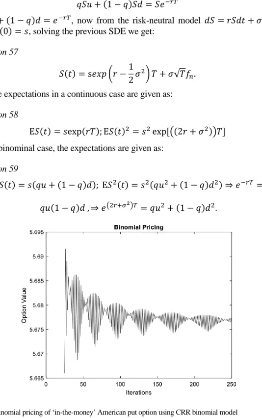
Fig. 1. Binomial pricing of ‘in-the-money’ American put option using CRR binomial model vs number of steps
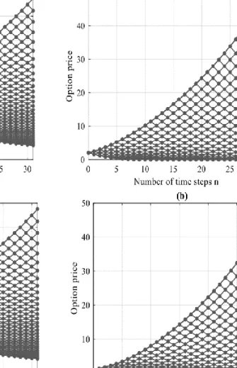
Fig. 2. Binomial lattice CRR model underlying price, and binomial lattice CRR option value model, Example 1 and Example 2
Source: authors’ own calculation.
The CRR model (1979) is a very popular model for evaluating American options and is referred to as the lattice model. This means that the underlying asset price can move up or down (two states) in some interval so the model is binomial. Convergence of the CRR formula to the Black-Scholes formula is proven by the central limit theorem. The previous result does not apply a triangular array of random variables, and the asymptotic distribution must be Gaussian.
Another possible model here is of Rendleman and Bartter (1979, 1980) who chose
Equation 60
𝑢 = 𝑒(𝑟−12𝜎2)𝑇+𝜎√𝑇; 𝑑 = 𝑒(𝑟− 1
2𝜎2)𝑇−𝜎√𝑇.
Stock price is an upper bound to the option price: 𝑐 ≤ 𝑆0 (Hull, 2017). An
American or European option gives the holder the right to sell one share of stock for 𝐾. No matter how low the stock price becomes, the option can never be worth more than 𝐾, so that: 𝑝 ≤ 𝐾. For European options, at maturity the option cannot be worth more than the present value of 𝐾: 𝑝 ≤ 𝐾 ∙ 𝑒−𝑟𝑇. A lower bound for the price on the
European call option on a non-dividend paying stock can be given as: 𝑆0∙ 𝐾 ∙ 𝑒−𝑟𝑇. In
the absence of arbitrage opportunities the following must apply:
Equation 61
𝑐 + 𝐾 ∙ 𝑒−𝑟𝑇≤ 𝑆0,
where 𝑐 represents the value of a European option to buy one share, and 𝑆0 represents
the current stock price, 𝐾strike price of option, and 𝑝 is the value of the European option to sell one share. By the put-call parity the portfolios must have identical values today: 𝑐 + 𝐾 ∙ 𝑒−𝑟𝑇= 𝑝 + 𝑆
0 . The RB model is intuitive and does not require a
higher level knowledge in probability theory, but the random variable is now the interest rate, which has implications on how discounting is done. Basically this model is a short rate model that defines the evolution of the interest rates.
4. The Leisen-Reimer model (1996)
Leisen and Reimer (1996) developed a model in order to improve the rate of convergence of their binomial tree model. All of the models discussed above converge to the Black-Scholes solution in the limit as the size of the time step Δ𝑡 is reduced to zero. However, the convergence is not smooth. The Leisen-Reimer model succeeded in defining a new binomial model where the option price converges smoothly to the Black-Scholes solution and they succeeded in achieving a second order convergence with a smaller error, namely the formulas to calculate (determine) the up and down factors change. Normally it is assumed that the asset follows a stochastic log-normal diffusion process, while in a simplified approach asset price changes are decomposed into Bernoulli steps which implies a time and state discrete replicating strategy. Convergence speed is measured by the order of convergence in the price approximations. The Leisen-Reimer (1996) model refers to the binomial tree option pricing models constructed by Cox, Ross and Rubinstein (1979), and Rendleman and Bartter (1980) binomial option pricing model. Leisen and Reimer (1996) employed the findings of the mathematics of normal approximations to the binomial function (namely, the Peizer and Pratt (1968), method for a normal approximation for binomial,
F, beta, and other common related tail probabilities). They also referred to that of Jarrow and Rudd (1983), which is termed the equal probability model. The Leisen- -Reimer model presents an attempt to improve the convergence speed of the CRR model that required too many steps. This model has an important advantage against the other models. The model has quadratic convergence in the number of time steps, while the other models have a linear convergence. The three models that Leisen- -Reimer (1996) compared are: the Cox-Ross-Rubinstein (1979), the Jarrow-Rudd (1983) and the Tian model (1993). Generally they find convergence in order one, so they conclude that the three above-mentioned models are equivalent. In short, they will be described after the table distribution and the lattice parameters.
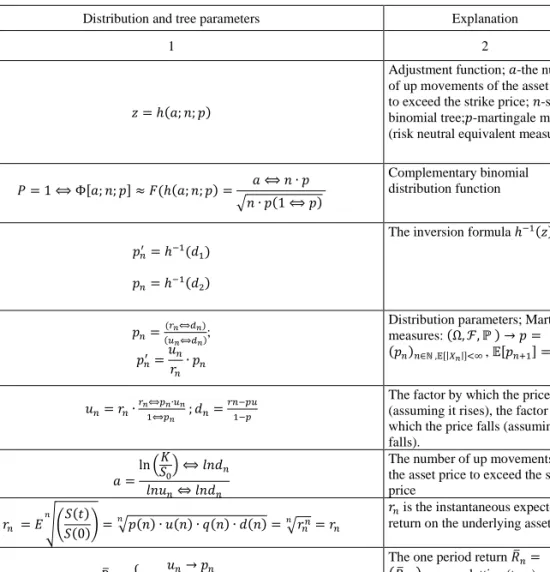
Table 1. Leisen-Reimer model parameters
Distribution and tree parameters Explanation
1 2
𝑧 = ℎ(𝑎; 𝑛; 𝑝)
Adjustment function; 𝑎-the number of up movements of the asset price to exceed the strike price; 𝑛-step binomial tree;𝑝-martingale measure (risk neutral equivalent measure)
𝑃 = 1 ⟺ Φ[𝑎; 𝑛; 𝑝] ≈ 𝐹(ℎ(𝑎; 𝑛; 𝑝) = 𝑎 ⟺ 𝑛 ∙ 𝑝 √𝑛 ∙ 𝑝(1 ⟺ 𝑝) Complementary binomial distribution function 𝑝𝑛′= ℎ−1(𝑑1) 𝑝𝑛= ℎ−1(𝑑2)
The inversion formula ℎ−1(𝑧) = 𝑝
𝑝𝑛= (𝑟𝑛⟺𝑑𝑛) (𝑢𝑛⟺𝑑𝑛); 𝑝𝑛′ = 𝑢𝑛 𝑟𝑛 ∙ 𝑝𝑛
Distribution parameters; Martingale measures: (Ω, ℱ, ℙ ) → 𝑝 = (𝑝𝑛)𝑛∈ℕ ,𝔼[|𝑋𝑛|]<∞ , 𝔼[𝑝𝑛+1] = 𝑝𝑛 𝑢𝑛= 𝑟𝑛∙ 𝑟𝑛⟺𝑝𝑛∙𝑢𝑛 1⟺𝑝𝑛 ; 𝑑𝑛= 𝑟𝑛−𝑝𝑢 1−𝑝
The factor by which the price rises (assuming it rises), the factor by which the price falls (assuming it falls).
𝑎 = ln (𝐾
𝑆0) ⟺ 𝑙𝑛𝑑𝑛
𝑙𝑛𝑢𝑛⇔ 𝑙𝑛𝑑𝑛
The number of up movements of the asset price to exceed the strike price 𝑟𝑛 = 𝐸 √( 𝑆(𝑡) 𝑆(0)) 𝑛 = √𝑝(𝑛) ∙ 𝑢(𝑛) ∙ 𝑞(𝑛) ∙ 𝑑(𝑛)𝑛 = √𝑟𝑛 𝑛𝑛= 𝑟𝑛
𝑟𝑛 is the instantaneous expected return on the underlying asset 𝑆
𝑅̅𝑛= {
𝑢𝑛→ 𝑝𝑛
𝑑𝑛→ 1 − 𝑝𝑛≡ 𝑞𝑛
The one period return 𝑅̅𝑛=
(𝑅̅𝑛,𝑖)𝑖=1,….𝑛 – lattice (tree)
𝑆̅𝑛,𝑘 = 𝑆0∙ ∏ 𝑅̅𝑛,𝑖 𝑘
𝑖=1
Table 1, cont.
Source: (Leisen and Reimer, 1996).
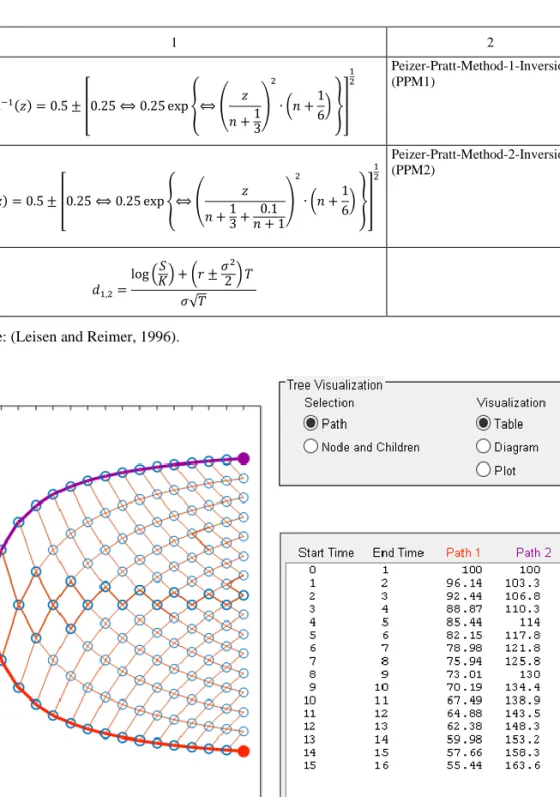
Fig. 3. The Leisen-Reimer Tree
Source: authors’ own calculation.
1 2 ℎ−1(𝑧) = 0.5 ± [0.25 ⟺ 0.25 exp {⟺ ( 𝑧 𝑛 +13 ) 2 ∙ (𝑛 +1 6) }] 1 2 Peizer-Pratt-Method-1-Inversion (PPM1) ℎ−1(𝑧) = 0.5 ± [0.25 ⟺ 0.25 exp {⟺ ( 𝑧 𝑛 +13+𝑛 + 10.1 ) 2 ∙ (𝑛 +1 6) }] 1 2 Peizer-Pratt-Method-2-Inversion (PPM2) 𝑑1,2= log (𝐾𝑆) + (𝑟 ±𝜎 2 2) 𝑇 𝜎√𝑇
Leisen and Reimer (1996) developed a model with the purpose of improving the rate of convergence of their binomial tree. This model is used in this paper since Leisen and Reimer succeeded in achieving order of convergence two with much smaller initial error.
5. The Tian model (1993)
This is the binomial model given in Tian (1993). It can be described by matching three moments in the Black-Scholes model with the binomial tree model, so that the three equations are: Equation 62 { 𝔼(𝑆Δ𝑡) = 𝑝𝑢 + (1 − 𝑝)𝑑 = 𝑒𝑟Δ𝑡 𝔼(𝑆Δ𝑡2) = 𝑝𝑢2+ (1 − 𝑝)𝑑2= (𝑒𝑟Δ𝑡)2𝑒𝜎 2Δ𝑡 𝔼(𝑆Δ𝑡3 ) = 𝑝𝑢3+ (1 − 𝑝)𝑑3 = (𝑒𝑟Δ𝑡)3𝑒𝜎 3Δ𝑡 ,
where 𝑟 and 𝜎 are the risk-free interest rate and the volatility in the Black-Scholes model. The unknowns in the models are given by the expression:
Equation 63 { 𝑝 =𝑒 𝑟Δ𝑡− 𝑑 𝑢 − 𝑑 ; 𝑢 =1 2𝑒 𝑟Δ𝑡𝑉 (𝑉 + 1 + √𝑉2+ 2𝑉 − 3 ) ; 𝑢 =1 2𝑒 𝑟Δ𝑡𝑉 (𝑉 + 1 − √𝑉2+ 2𝑉 − 3) .
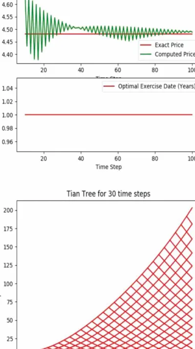
In the previous expression also 𝑉 = 𝑒𝜎2Δ𝑡 and 𝑒𝑟Δ𝑡= 𝑀. The next plot shows the convergence of the Tian model, and in the second graph the optimal exercise time. The Tian model parameters are: 𝑆0= 100; 𝜎 = 0.2; 𝑟 = 0.006; 𝐾 = 110; 𝑇 = 1;
𝐵 = 110; time steps are 𝑁𝑚𝑖𝑛 = 10 → 𝑁𝑚𝑎𝑥= 110; 𝜀 = 0.1; 𝑁𝑟𝑒𝑓 = 30, used in
the construction of a reference tree of size 𝑁𝑟𝑒𝑓 (the last graph B).
The Tian model (1993) exactly matches the first three moments of the binomial model to the first three moments of a lognormal distribution. In the model two equations are given that ensure that over a small period the expected mean and variance of the binomial model will match those expected in a risk neutral world.
Fig. 4. Convergence to the BS model of the Tian result and the Tian Tree Source: authors’ own calculation.
6. The Jarrow-Rudd model (1983)
This model is based on a log-normal transformation of the binomial model, hence we allow for: 𝑌Δ𝑡 = 𝑙𝑜𝑔(𝑆Δ𝑡). Due to the BSM, 𝑌Δ𝑡 ∼ 𝒩(𝑌0+ 𝛾Δ𝑡 , 𝜎2Δ𝑡) and now we
set: 𝛾 = 𝑟 −𝜎2 2 to obtain: Equation 64 {𝔼(𝑌Δ𝑡) = 𝑌0+ 𝛾Δ𝑡 𝕍𝑎𝑟(𝑌Δ𝑡2) = 𝜎2Δ𝑡 . Then if we set 𝑝 =1 2 we obtain: Equation 65 { 𝔼(𝑌Δ𝑡) = 𝑌0+ ln(𝑢𝑑) 2 𝕍𝑎𝑟(𝑌Δ𝑡2) =1 4(ln ( 𝑢 𝑑)) 2 .
By matching the first two we arrive at:
Equation 66 { 𝑝 =1 2 𝑢 = 𝑒(𝑟2− 𝜎2 2)Δ𝑡+𝜎√Δ𝑡 𝑑 = 𝑒(𝑟2− 𝜎2 2)Δ𝑡−𝜎√Δ𝑡 .
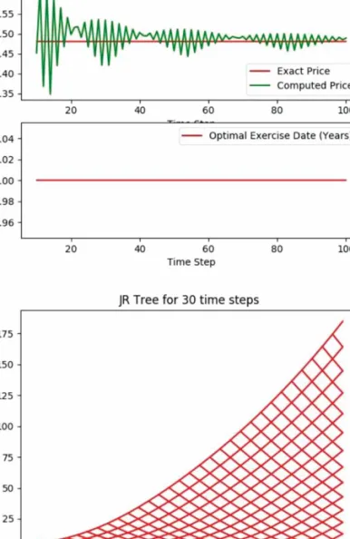
Thus the next plot shows the convergence of the Jarrow-Rudd model, and the second graph the optimal exercise time. The Jarrow-Rudd model parameters are:
𝑆 = 100; 𝜎 = 0.2; 𝑟 = 0.006; 𝐾 = 110; 𝑇 = 1; 𝐵 = 110; time steps are: 𝑁𝑚𝑖𝑛 =
10 → 𝑁𝑚𝑎𝑥= 110; 𝜀 = 0.1; 𝑁𝑟𝑒𝑓 = 30, used in the construction of a reference tree
of size 𝑁𝑟𝑒𝑓 (the last graph B).
The Jarrow-Rudd model (1983) says that the resulting option price is expressed as the sum of a Black-Scholes price plus adjustment terms which depend on the second and higher moments of the underlying security stochastic process. In this model underlying security distribution is log-normal.
Fig. 5. Convergence of the Jarrow-Rudd model and the JR Tree Source: authors’ own calculation.
7. The Trigeorgis Model (1991)
The Trigerogis model (1991), is based on a log-transformation of the Black-Scholes model and is designed to overcome the problems of stability, consistency and efficiency encountered in the Cox, Ross and Rubinstein model (1979). We set:
𝑌Δ𝑡 = 𝑙𝑜𝑔(𝑆Δ𝑡) . Due to the BSM we know that: 𝑌Δ𝑡 ∼ 𝒩(𝑌0+ 𝛾Δ𝑡 , 𝜎2Δ𝑡) and now
we set: 𝛾 = 𝑟 −𝜎2
2 and then obtain:
Equation 67
{ 𝔼(𝑌Δ𝑡) = 𝑌0+ 𝛾Δ𝑡
𝔼(𝑌Δ𝑡2) = 𝑌02+ (𝜎2+ 2𝛾𝑌0)Δ𝑡 + 𝛾2Δ𝑡2.
Since 𝑢 =1
𝑑 and 𝑙𝑜𝑔𝑑 = − log(𝑢) on the binomial tree we obtain:
Equation 68
{ 𝔼(𝑌Δ𝑡) = 𝑌0+ (2𝑝 − 1) log(𝑢) ; 𝔼(𝑌Δ𝑡2) = 𝑌02+ 2(2𝑝 − 1)(𝑙𝑜𝑔𝑢)𝑌0+ (𝑙𝑜𝑔𝑢)2
.
By matching the previous two moments one obtains the model equations:
Equation 69 { 𝑢 =1 𝑑; 𝛾Δ𝑡 = (2𝑝 − 1) log(𝑢) (𝜎2+ 2𝛾)Δ𝑡 + 𝛾2Δ𝑡2= 2(2𝑝 − 1)(𝑙𝑜𝑔𝑢)𝑌 0+ (𝑙𝑜𝑔𝑢)2
and by solving the previous equations:
Equation 70 { 𝛾 = 𝑟 −𝜎 2 2 ; 𝑥 = √𝜎2Δ𝑡 + 𝛾2Δ𝑡2; 𝑢 = 𝑒𝑥; 𝑑 =1 𝑢= 𝑒 −𝑥; 𝑝 =1 2(1 + 𝛾Δ𝑡 𝑥 ) .
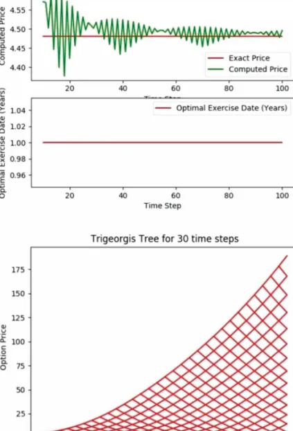
The next plot shows the convergence of the Trigeorgis model and the second graph, the optimal exercise time. The Trigeorgis model parameters are: 𝑆0= 100;
𝜎 = 0.2; 𝑟 = 0.006; 𝐾 = 110; 𝑇 = 1; 𝐵 = 110; time steps are 𝑁𝑚𝑖𝑛 = 10 →
𝑁𝑚𝑎𝑥 = 110; 𝜀 = 0.1; 𝑁𝑟𝑒𝑓= 30, used in the construction of a reference tree of size
Fig. 6. Convergence to the BS model of Trigeorgis and the Trigeorgis Tree Source: authors’ own calculation.
The Trigeorgis model (1991), is a log-transformed variation of binomial option pricing designed to overcome the problem of consistency, stability and efficiency encountered by the CRR (1979) model. This model also shows that risk neutral probability in the log-transformed binomial mode converges to that of the CRR model.
8. Convergence of the lattice methods
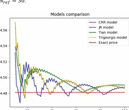
The next plot shows the convergence of the four models, and the table the optimal number of steps in convergence. The models’ parameters are: 𝑆0= 100; 𝜎 = 0.2;
𝑟 = 0.006; 𝐾 = 110; 𝑇 = 1; 𝐵 = 110; time steps are 𝑁𝑚𝑖𝑛 = 10 → 𝑁𝑚𝑎𝑥 =
110; 𝜀 = 0.1; 𝑁𝑟𝑒𝑓= 30.
Fig. 7. Models comparison Source: authors’ own calculation.
Table 2. Number of convergence steps comparison
Model CRR JR Tian Trigeorgis
𝑁-number of convergence steps
19 16 19 19
Source: authors’ own calculation.
Trinomial option pricing models
Here the authors compare convergence of the previously explained binomial models: CRR (1979) and Tian (1993), to the binomial Haahtela (2010), trinomial Boyle (1986, 1988), and Kamrad-Ritchken model (1991). The trinomial models in general have: up, down and middle stable path. The stock price ratio 𝑆𝑖+1
𝑆𝑖 takes the value 𝑑, 𝑚, 𝑢 and 𝑑 < 𝑚 < 𝑢 and the assigned probabilities are: 𝑝𝑑, 𝑝𝑚, 𝑝𝑢. In
Equation 71
𝑢 = 𝑒𝑟∙Δ𝑡+√𝑒(𝜆𝜎)2Δ𝑡−1 ; 𝑑 = 𝑒𝑟∙Δ𝑡−√𝑒(𝜆𝜎)2Δ𝑡−1 ; 𝑞 = (𝑟 − d 𝑢 − 𝑑).
In this model we set 𝜆 = 1 so that the trinomial model behaves as, and becomes binomial. If 𝜆 = 1.50.5≈ 1.22, transition probabilities all converge to 1/3, when
Δ𝑡 → 0 .
9. The Haahtela model (2010)
In Haahtela (2010), the model probabilities and transition probabilities and risk neutral state transition 𝑞′𝑠 probabilities are given as:
Equation 72 { 𝑝𝑢 = 𝑚2(𝑉 − 1) 𝑢2+ 𝑚𝑑 − 𝑢𝑚 − 𝑢𝑑 𝑝𝑑 = 𝑝𝑢( 𝑢 − 𝑑 𝑑 − 𝑚) 𝑝𝑚 = 1 − 𝑝𝑢− 𝑝𝑑 ; { 𝑝𝑢𝑖 = 𝑝 𝑢( 𝜎𝑖 𝜎𝑚𝑎𝑥 ) 2 𝑝𝑑𝑖 = 𝑝𝑑( 𝜎𝑖 𝜎𝑚𝑎𝑥 ) 2 𝑝𝑚𝑖 = 1 − 𝑝𝑢𝑖 − 𝑝𝑑𝑖 ; 𝑞1= 𝑒𝑟∙Δ𝑡 − 𝑑 𝑢 − 𝑑 ; 𝑞2= 1 − 𝑞1, where 𝑀 = 𝑒𝑟Δ𝑡 ; 𝑉 = 𝑒𝜎2Δ𝑡, and 𝜎 𝑖 = √ln(𝑆𝑒𝑟𝑡 √ 𝑒∑𝜎𝑖2𝑡𝑖−1 𝑆0𝑒𝑟𝑡 )−∑1𝑖=0(𝜎𝑖2𝑡𝑖) 𝑡𝑖 , and standard
deviation is given as: 𝑆𝑡𝑑 = 𝑆𝑒𝑟𝑡√𝑒∑𝜎𝑖2𝑡𝑖− 1 . Ans 𝑚 = 𝑟 ∙ (𝑒𝜎2∙Δ𝑡 )2= 𝑒𝑟∙Δ𝑡∙
(𝑒𝜎2∙Δ𝑡 )2 now when Δ𝑡 → 0 then 𝑚 = 1. This model presents a recombining trinomial tree for valuing real options with changing volatility, where volatility changes are modelled with the changing transition probabilities, that could be changing.
10. The Boyle (1986) model
In (Boyle 1986), the model movement scales and transitive probabilities are given as:
{
𝑢 = 𝑒
𝜆𝜎√𝛥𝑡
𝑚 = 1
𝑑 = 𝑒
−𝜆𝜎√𝛥𝑡{ 𝑝𝑢= (𝑒𝑥𝑝(2𝑟 + 𝜎2) 𝛥𝑡 ) − 𝑒𝑥𝑝(𝑟𝛥𝑡 ) − (𝑒𝑥𝑝(𝑟𝛥𝑡 ) − 1) (𝑒𝑥𝑝(𝜆𝜎√𝛥𝑡) − 1)(𝑒𝑥𝑝(2𝜆𝜎√𝛥𝑡 ) − 1) 𝑝𝑚 = 1 − 𝑝𝑢− 𝑝𝑑 𝑝𝑑 = (𝑒𝑥𝑝(2𝑟 + 𝜎2) 𝛥𝑡 ) − 𝑒𝑥𝑝(𝑟𝛥𝑡 )(𝑒𝑥𝑝(2𝜆𝜎√𝛥𝑡 )) − (𝑒𝑥𝑝(𝑟𝛥𝑡 ) − 1) (𝑒𝑥𝑝(𝜆𝜎√𝛥𝑡) − 1)(𝑒𝑥𝑝(2𝜆𝜎√𝛥𝑡 ) − 1) .
Risk-neutral state transition probabilities (see Bowei and Wang 2015) are given as:
Equation 73 { 𝑞1 = (𝜁 + 𝛾2− 𝛾)𝑢 − (𝛾 − 1) (𝑢2− 1) (𝑢 − 1) 𝑞2= 1 − 𝑞1− 𝑞3; 𝑞3= (𝜁 + 𝛾2− 𝛾)𝑢2− (𝛾 − 1)𝑢3 (𝑢2− 1) (𝑢 − 1) ,
where the previous expression 𝜁 = 𝑒2𝑟Δ𝑡(𝑒𝜎2Δ𝑡− 1) and 𝛾 = 𝑒𝑟Δ𝑡. In the Boyle
(1986) trinomial lattice model, the asset price can either move upwards, downwards, or stay unchanged in a given time period.
11. The Kamrad-Ritchken model (1991)
In the Kamrad-Ritchken or K-R model (1991), movement scales , risk neutral state transition q's probabilities are given as:
Equation 74 {𝑢 = 𝑒 𝜆𝜎√Δ𝑡 𝑚 = 1 𝑑 = 𝑒−𝜆𝜎√Δ𝑡 ; { 𝑞1= 1 2𝜆2+ (𝑟 −12 𝜎2) √Δ𝑡 2𝜆𝜎 𝑞2= 1 − 1 𝜆2 𝑞3= 1 2𝜆2− (𝑟 −12 𝜎2) √Δ𝑡 2𝜆𝜎 .
The Kamrad-Ritchken model is a trinomial tree with 2𝑛 + 1 possible values of the underlying security throughout the option life. The Kamrad-Ricthken tree coincides with the explicit difference scheme, except that it treats differently the discount factors in the B-S scheme (𝑟 and 𝑢).
12. The trinomial Tian model
In the trinomial Tian (1993) models, movement scales and transition probabilities are given as: Equation 75 { 𝑢 = 𝜔̅ + √𝜔̅2− 𝑚2; 𝜔̅ =𝛾 2(𝜁 4+ 𝜁3) 𝑚 = 𝛾𝜁2; 𝛾 = 𝑒𝑟Δ𝑡; 𝜁 = 𝑒𝜎2Δ𝑡 𝑑 = 𝜔̅ − √𝜔̅2− 𝑚2 ; { 𝑞1= 𝑚𝑑 − 𝛾(𝑚 + 𝑑) + 𝛾2𝜁 (𝑢 − 𝑑)(𝑢 − 𝑚) 𝑞2= 𝛾(𝑢 + 𝑑) − 𝑢𝑑 − 𝛾2𝜁 (𝑢 − 𝑚)(𝑢 − 𝑑) 𝑞3= 𝑢𝑚 − 𝛾(𝑢 + 𝑚) + 𝛾2𝜁 (𝑢 − 𝑑)(𝑚 − 𝑑) .
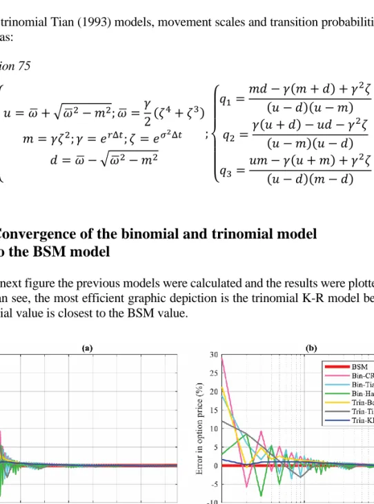
13. Convergence of the binomial and trinomial model
to the BSM model
In the next figure the previous models were calculated and the results were plotted. As one can see, the most efficient graphic depiction is the trinomial K-R model because its initial value is closest to the BSM value.
Fig. 8. Number of iterations and convergence of binomial and trinomial models Source: authors’ own calculation.
14. Conclusion
In this paper the authors presented the two most basic forms of lattice models of option valuation-the binomial and trinomial approaches, and also described the derivations of the selected and presented model and their movement scales and transitive probabilities. The paper examined the convergences of these models in the European call option case. A European option is a financial contract that gives the holder a right but not an obligation to buy and sell the underlying asset from the writer at the time of expiry for a pre-determined price. The continuous model of the European call option is given by the Black-Scholes model, while discrete models are those models that can be priced by using the lattice models binomial and trinomial (see: Puspita, Agustina, and Sispiyati, 2013). Here, the error is defined as the difference between the binomial or trinomial approximation and by the value computed by the BS formula. This case considered the convergence on two occasions: the first of the binomial lattice models, the Cox-Ross-Rubinstein, Jarrow-Rudd, Tian and Trigeorgis models, to the true value BS model. Firstly, the authors discovered that for the European call option valuation, the Jarrow-Rudd model achieves the fastest convergence in 16 steps, while all the other models achieved the convergence in 19 steps. Secondly, the authors compared the binomial and trinomial lattice models, and examined the convergence to the Black-Scholes-Merton model. Then the computation of the option value by the models determined that the most efficient model for option pricing is the trinomial K-R model or the trinomial Kamrad-Ritchken model, second best is the binomial Haahtela model, followed by the trinomial Tian model, and other binomial models. Thus, in conclusion, European option pricing using trinomial models converges more quickly to the European Black-Scholes option pricing as compared to the binomial option pricing.
The topic of speed of convergence of binomial and trinomial is of importance in the real world since the difference in the convergence of option prices (their trading value) to their fundamental value, determines the size of the bubbles (if there exists a gap between the two, it is by definition a trading bubble). The results confirmed that the Jarrow-Rudd model, or equal probability model, achieves the fastest convergence for the European call option. From the trinomial lattice (discrete time) model, the Kamrad-Ritchken model (1991) proves to be of lowest order of convergence and is fastest for the European call option. The binomial CRR model in the case of the American call option reported 30 steps until convergence.
References
Akerlof, G. (2002). Behavioral macroeconomics and macroeconomic behavior. The American Economic Review, 92(3), 411-433.
Bates, D. (1996). Jumps and stochastic volatility: Exchange rate processes implicit in Deutschemark options. Review of Financial Studies, (9), 69-108.
Black, F., and Scholes, M. (1973). The pricing of options and corporate liabilities. The Journal of Political Economy, 81(3), 637-654.
Bowei, C., and Wang, J. ( 2015). A lattice framework for pricing display and options with the stochastic volatility model. Electronic Commerce Research and Applications, 14(6), 465-479.
Boyle, P. (1986). Option valuation using a three-jump process. International Options Journal, (3), 7-12. Boyle, P. (1988). A lattice framework for option pricing with two state variables. Journal of Financial
and Quantitative Analysis, 3, 1-12.
Campbell, J., and Shiller, R. J. (1987). Cointegration and tests of present value models. Journal of Political Economy, (97), 1062-1088.
Carr, P., and Madan, B. D. (1999). Option valuation using the fast Fourier transform. Quantitative Finance, (1), 19-37.
Cootner, P. H. (1964). The random character of stock market prices. Cambridge, Mass.: MIT Press. Cox, J. C., and Ross, S. A. (1975). The pricing of options for Jump processes. Rodney L. White Center
for Financial Research (Working Paper No. 2-75). University of Pennsylvania, Philadelphia, PA. Cox, J. C., and Ross, S. A. (1976). The valuation of options for alternative stochastic processes. Journal
of Financial Economics, (3), 145-166.
Cox, J. C., Ross, S. A., and Rubinstein, M. (1979). Option pricing: A simplified approach. Journal of Financial Economics, 7(3), 229.
Fama, E. (1970). Efficient capital markets: A review of theory and empirical work. Journal of Finance,
25(2), 383-417.
Gurdip, B., and Chen, Z. (1997). An alternative valuation model for contingent claims. Journal of Financial Economics, 44(1), 123-165.
Haahtela, T. (2010). Recombining trinomial tree for real option valuation with changing volatility. Aalto University (Working Paper Series).
Heston, S. (1993). A closed-form solution for options with stochastic volatility with applications to bond and currency options. Review of Financial Studies, (6), 327-343.
Hull, J. C. (2017). Options, Futures, and Other Derivatives, Pearson. Jarrow, R., and Rudd, A. (1983). Option pricing. Homewood, Illinois.
Kamrad, B., and Ritchken, P. (1991). Multinomial approximating models for option with k states variables. Management Sciences, 37(23), 1640-1652.
Kiyosi, I. (1944). Stochastic integral. Proc. Imperial Acad. Tokyo, (20), 519-524.
Leisen, D., and Reimer, M. (1996). Binomial models for option valuation – examining and improving convergence. Applied Mathematical Finance, 3(4), 319-346.
Merton, R. C. (1973), Theory of rational option pricing. Bell Journal of Economics, 4(1), p. 141-183. Merton, R. C. (1973a). Continuous-time speculative processes': Appendix to Paul A. Samuelson's
'mathematics of speculative price'. SIAM Review 15 (January 1973), 34-38.
Merton, R. C. (1973b). An intertemporal capital asset pricing model. Econometrica, 41(5), 867-887. Merton, R. C. (1973c). The relationship between put and call option prices: Comment. Journal of
Finance, 28(1), 183-184.
Merton, R. C. (1975). Option pricing when underlying stock returns are discontinuous. Journal of Financial Economics, (3), 125-144.
Merton, R. C., and Samuleson, P. (1974). Fallacy of the log-normal approximation to optimal portfolio decision-making over many periods. Journal of Financial Economics, 1(1), 67-94.
Peizer, D. B., and Pratt, J. W. (1968). A normal approximation for binomial, f, beta, and other common related tail probabilities, I, The Journal of the American Statistical Association, (63), 1416-1456. Pratt, J. W. (1968). A normal approximation for binomial, f, beta, and other common, related tail
probabilities, II. The Journal of the American Statistical Association, (63), 1457-1483.
Puspita, E., Agustina, F., and Sispiyati, R. (2013). Convergence numerically of trinomial model in European option pricing. International Research Journal of Business Studies, 6(3), 195-201. Rendleman, R., and Bartter, B. (1979). Two-state option pricing. Journal of Finance, (24), 1093-1110. Rendleman, R., and Bartter, B. (1980). The pricing of options on debt securities. Journal of Financial
Romer, D. H. (1993). Rational asset-price movements without news. The American Economic Review,
83(5), 1112-1130.
Ross, S., (1976). The arbitrage theory of capital asset pricing. Journal of Economic Theory, 13(3), 341--360. doi:10.1016/0022-0531(76)90046-6
Samuelson, P. A. (1965). Rational theory of warrant pricing. Industrial Management Review, (6), 13-31. Scott, L. (1997). Pricing stock options in a jump-diffusion model with stochastic volatility and interest
rates: Application of Fourier inversion methods. Mathematical Finance, (7), 413-426. Smith, C. W. (1976). Option pricing: A review. Journal of Financial Economics, 3(1-2), 3-51. Tian, Y. (1993). A modified lattice approach to option pricing. Journal of Futures Markets, 13(5), 563-577. Trigeorgis, L. (1991). A log-transformed binomial analysis method for valuing complex multi-option
investments. Journal of Financial and Quantitative Analysis, 26(3), 309-326.
Wilmott, P., Howison, S., and Dewynne, J. (1997). The mathematics of financial derivatives: A student introduction (2 ed.). Cambridge University Press.
PRZEGLĄD DWUMIANOWYCH I TRÓJMIANOWYCH MODELI
WYCENY OPCJI I ICH ZBIEŻNOŚĆ DO MODELU BLACKA-SCHOLESA OKREŚLAJĄCEGO WYCENĘ OPCJI
Streszczenie: W artykule dokonano przeglądu modeli wyceny opcji dwumianowych i trójmianowych oraz ich zbieżności z wynikami zastosowania modelu Blacka-Scholesa (BS). Przeprowadzono uogólnienie modeli dla opcji europejskich i amerykańskich. W literaturze wskazuje się, że modele trójmianowe w przypadku mniejszej liczby kroków dają bardziej dokładne wyniki niż modele dwumianowe. Modele te są szeroko stosowane dla zwykłych typów opcji waniliowych, opcji europejskich lub amerykańskich, które odpowiednio można wykonać tylko w dniu wygaśnięcia i w dowolnym momencie przed datą wygaśnięcia. Otrzymane wyniki potwierdzają konwencjonalną teorię, że trójmianowe modele wyceny opcji, takie jak model Kamrada-Ritchkena i model Boyle’a, są szybciej zbieżne niż modele dwumianowe. W porównaniu modeli dwumianowych pod względem konwergencji najbardziej efektywnym modelem jest model Jarrowa-Rudda. W artykule zapre-zentowano wyniki wskazujące, że ulepszone modele dwumianowe, takie jak model Haahtela, są szybciej zbieżne do wyników uzyskanych z modelu BS. Po przeprowadzeniu kilku prób wskazano, że rozkład dwumianowy jest zgodny z rozkładem logarytmiczno-normalnym przyjętym przez model Blacka-Scholesa.
Słowa kluczowe: modele: Blacka-Scholesa-Mertona, Leisena-Reimera, Coxa-Rossa-Rubinsteina, Tiana, Trigeorgisa.
Quote as: Josheski, D., Apostolov, M. (2020). A review of the binomial and trinomial models for option pricing and their convergence to the Black-Scholes model determined option prices.
Econometrics. Ekonometria. Advances in Applied Data Analysis, 24(2).