University of Rhode Island University of Rhode Island
DigitalCommons@URI
DigitalCommons@URI
Open Access Master's Theses2013
Networked Differential GPS Methods
Networked Differential GPS Methods
Simon P. BarrUniversity of Rhode Island, [email protected]
Follow this and additional works at: https://digitalcommons.uri.edu/theses
Recommended Citation Recommended Citation
Barr, Simon P., "Networked Differential GPS Methods" (2013). Open Access Master's Theses. Paper 28. https://digitalcommons.uri.edu/theses/28
NETWORKED DIFFERENTIAL GPS METHODS BY
SIMON P. BARR
A THESIS SUBMITTED IN PARTIAL FULFILLMENT OF THE REQUIREMENTS FOR THE DEGREE OF
MASTER OF SCIENCE IN
ELECTRICAL ENGINEERING
MASTER OF SCIENCE THESIS OF
SIMON P. BARR
APPROVED:
Thesis Committee:
Major Professor Dr. Peter F. Swaszek
Dr. Richard J. Hartnett
Dr. Manbir S. Sodhi
Dr. Nasser H. Zawia
DEAN OF THE GRADUATE SCHOOL
ABSTRACT
Historically, maritime organizations seeking accurate shipboard positioning have relied upon some form of differential GNSS, such as DGPS, WAAS, or EGNOS, to im-prove the accuracy and integrity of the GPS. Ground-based augmentation systems, such as DGPS, broadcast corrections to the GPS signal from geographically distributed ter-restrial reference stations—often called beacons. Specifically, pseudorange corrections to the GPS L1 C/A signal are computed at each reference site, then broadcast in the nearby geographic area using a medium frequency (approximately 300 kHz) communi-cations link. The user then adds these corrections onto their measured pseudoranges before implementing a position solution algorithm. Within the United States, the U.S. Coast Guard operates 86 DGPS reference beacons. Similar DGPS systems are operated in Europe and elsewhere around the globe.
While current DGPS receiver algorithms typically use one set of pseudorange cor-rections from one DGPS reference site (often the one with the “strongest” signal), many user locations can successfully receive two or more different DGPS broadcasts. This suggests two obvious questions: “If available, how does one select the corrections to use from multiple sets of corrections?” and “Is it advantageous to combine corrections in some way?” A number of factors might influence the effectiveness of any particular station’s corrections. Some of these refer to the effectiveness of the communications link itself, including concerns about interference from other beacons (skywave interfer-ence from far-away beacons on similar frequencies, a notable problem in Europe) and self-interference (skywave fading). Other factors refer to the accuracies of pseudorange corrections: for example, ionospheric storm-enhanced plasma density (SED) events can cause the corrections to have large spatial variation, making them poor choices even for users close to a beacon.
Earlier work in the area of DGPS beacon selection has identified several options, including choosing the beacon closest to the user or the beacon with the least skywave interference. There have also been suggestions on how to combine corrections when
corrections, where the weights are typically inversely proportional to the distance from the user to the individual beacon.
This thesis re-examines the concept of multi-beacon DGPS by evaluating methods of combining beacon corrections based on spatial relativity. Recent research determines that DGPS accuracy performance is biased: the mean scatter of DGPS-corrected po-sitions does not fall on the true receiver position. This finding was re-established this using networked DGPS methods both by processing GPS L1 C/A observables from dozens of CORS (Continuously Operating Reference Station) sites around the U.S.A. and via simulation using a Spirent GSS8000 GPS simulator. Specifically, we found that (a) the position solution computed using DGPS beacon corrections is typically biased in a direction away from the beacon and (b) the magnitude of the bias depends upon the distance from the beacon. This bias grows with a slope of approximately one-third of a meter per 100 km of user-to-beacon distance. We also found that networking DGPS corrections decreases the errors of bias magnitude and scatter radius inherent in single-beacon solutions.
This thesis compares the performance of several multi-beacon algorithms assessed using both GPS simulator and real-world data. These algorithms include simple aver-aging, a weighted sum based on inverse-range to each beacon, a weighted sum based on inverse-range-squared to each beacon, and spatial linear interpolation correction. Spatial linear interpolation factors in distances and angles to the known locations of the DGPS transmitters.
As part of this research effort, we developed a DGPS receiver using a software-defined radio platform. Ettus Research’s USRP was chosen as the SDR device to collect and digitize GPS and DGPS radio signals. For the real-world tests, we applied networked DGPS pseudorange corrections to post-processed CORS data. The results of these tests confirm the spatial behavior of the simulator trials with respect to bias magnitude and scatter radius. A complete description of this system is included in the thesis.
ACKNOWLEDGMENTS
I would like to highlight the numerous contributions to this research by my advi-sor, Dr. Peter Swaszek. His in-depth knowledge of GPS, Differential GPS and signal processing methods have proved invaluable to me throughout the course of this work.
I would like to thank the other members of my committee, Dr. Richard Hartnett from the U.S. Coast Guard Academy; Dr. Manbir Sodhi from the Department of Mechanical, Industrial, and Systems Engineering; and Dr. Robert Tyce from the Department of Ocean Engineering for taking time from their busy schedules in order to further my education.
I would also like to thank the faculty of the U.S. Coast Guard Academy, whose scholarly and material support have greatly assisted in the completion of this thesis. Dr. Richard Hartnett was both a source of motivation and information—whose wealth of knowledge in the area of Coast Guard radionavigation systems is unparalleled. Com-mander Joe Staier and ComCom-mander Rob Oatman subsidized both my time and material resource requirements with good humor and sacrificed nearly 4000 pounds of peanut M&M’s. Lieutenant Steve Myers expedited the purchase of specific equipment necessary for my research and Lieutenant Matt Kempe forfeited numerous servers, hard drives, and untold hours keeping my research bandwidth requirements satiated. Senior Chief Electronics Technician Ken McKinley provided technical expertise to set up and improve the infrastructure used to conduct this research.
Many thanks are deserved by those who—for no reason other than curiosity— persistently took the time to assist my research efforts. Tim Toolan was of great help in providing access to URI facilities and expertise with Linux, Jim Daly provided a number of material resources necessary to modify my equipment, and Andrew Cavanaugh helped lug test equipment all over the WPI campus.
Finally, I would like to thank Meredith Leach Sanders and Melyssa Lennox, who were able to make each day on campus much more interesting while simultaneously keeping the ECBE Department running. Turn to!
TABLE OF CONTENTS ABSTRACT . . . ii ACKNOWLEDGMENTS . . . iv TABLE OF CONTENTS . . . v LIST OF TABLES . . . ix LIST OF FIGURES . . . x CHAPTER 1 Introduction . . . 1
1.1 Overview of the Global Positioning System . . . 1
1.2 Overview of U.S. Coast Guard Differential GPS . . . 3
1.3 Impetus for current work . . . 5
1.4 Discussion of related work . . . 7
List of References . . . 8
2 Networked DGPS Methods . . . 10
2.1 Background . . . 10
2.2 Pseudorange calculation and correction . . . 10
2.3 Networking algorithms . . . 11
2.3.1 Simple averaging . . . 11
2.3.2 Inverse-range . . . 11
2.3.3 Inverse-range-squared . . . 12
2.3.4 Spatial linear interpolation (SLI) . . . 12
Page
3.1 Applicable software . . . 16
3.2 Simulator testing overview . . . 16
3.3 Simulator testing results . . . 22
3.4 Discussion of simulator results . . . 28
List of References . . . 32
4 Characterizing Networked DGPS Algorithm Performance . . . 33
4.1 Overview . . . 33
4.2 Characterizing spatial behavior . . . 33
4.2.1 Performance versus distance . . . 34
4.2.2 Performance versus azimuth . . . 40
4.3 Consideration of assumptions . . . 47
4.3.1 Assumption 1: Known satellite orbit . . . 48
4.3.2 Assumption 2: Zero clock bias . . . 48
4.3.3 Assumption 3: Sufficient atmospheric models . . . 49
4.3.4 Assumption 4: Zero multipath error . . . 50
4.3.5 Assumption 5: Zero thermal noise . . . 50
4.4 Consideration of noise . . . 51
4.4.1 Derivation of noise effects on DGPS . . . 52
4.4.2 Spatial representations of bias magnitude and noise covariance 56 4.5 Beacon grouping quality and selection criteria . . . 64
4.6 Discussion of Networked DGPS character . . . 68
List of References . . . 69
5 Real-World Implementation of Networked DGPS . . . 71
Page
5.3 The Universal Software Radio Peripheral . . . 73
5.3.1 USRP Hardware . . . 74
5.3.2 USRP Software . . . 78
5.4 Acquisition of DGPS and GPS signals . . . 84
5.4.1 DGPS signal acquisition . . . 84
5.4.2 GPS signal acquisition . . . 87
5.5 Networked DGPS with MATLAB . . . 92
5.6 CORS processing with MATLAB. . . 93
List of References . . . 99
6 Considerations and Conclusions . . . 100
6.1 Other considerations . . . 100 6.2 Future work . . . 101 6.3 Conclusions . . . 102 APPENDIX A System Configuration . . . 104 A.1 Purpose . . . 104
A.2 Ettus Research USRP . . . 104
A.3 Receiving equipment . . . 104
A.4 USRP client computer . . . 105
A.5 USRP blade server . . . 105
List of References . . . 106
B USRP N210 Setup on Ubuntu 12.04 x64 . . . 107
Page
B.3 Establish USRP IP-Layer Communication . . . 107
B.4 Build USRP UHD 003.002.003 . . . 109
B.5 Build GnuRadio with UHD Blockset . . . 112
C USRP N210 Setup on MATLAB R2012a . . . 116
C.1 Purpose . . . 116
C.2 Establish USRP IP-Layer Communication . . . 116
C.3 Install the USRP Support Package in MATLAB . . . 118
D List of Abbreviations . . . 120
E List of Symbols . . . 122
LIST OF TABLES
Table Page
4.1 Linear coefficients of 2drms performance over distance south from
Moriches, NY, by beacon grouping . . . 36
5.1 USRP N210 daughterboard functions and capabilities . . . 75
5.2 GPS signal correlation to PRN sequences 1–32 . . . 91
A.1 Major components and capabilities of the USRP N210 . . . 104
LIST OF FIGURES
Figure Page
1.1 Typical DGPS implementation . . . 4
1.2 Multi-beacon coverage map of continental U.S.A. . . 5
1.3 Bias magnitude and scatter radius spatial decorrelation plots . . . 7
3.1 Total atmospheric correction plot over New England . . . 17
3.2 Map of simulator testing locations . . . 18
3.3 Map of Long Island Sound transit . . . 19
3.4 Representations of networking DGPS methods . . . 20
3.5 SLI comparison to “actual” PRCs . . . 21
3.6 Simulator position plots of beacon/rover group 1A . . . 23
3.7 Simulator position plots of beacon/rover group 1B . . . 23
3.8 Simulator position plots of beacon/rover group 1C . . . 24
3.9 Simulator position plots of beacon/rover group 1D . . . 24
3.10 Simulator position plots of beacon/rover group 1E . . . 25
3.11 Simulator position plots of beacon/rover group 1LIS . . . 25
3.12 Simulator position plots of beacon/rover group 2D . . . 26
3.13 Simulator position plots of beacon/rover group 2E . . . 26
3.14 Simulator position plots of beacon/rover group 2F . . . 27
3.15 Simulator position plots of beacon/rover group 2LIS . . . 27
3.16 Bias length, 95% scatter radius, and2drms comparison bar graphs . 31 3.17 Satellite count for Group-Point 1E . . . 31
4.1 Map of 2drms distance testing locations . . . 37
Figure Page
4.3 2drmsvs. distance east of Moriches, NY . . . 39
4.4 Map of 2drms radial testing locations from Group 1 . . . 42
4.5 2drmsvs. azimuth from Group 1 centroid . . . 43
4.6 Map of 2drms radial testing locations from Group 2 . . . 44
4.7 2drmsvs. azimuth from Moriches, NY at 100-km radius . . . 45
4.8 2drmsvs. azimuth from Moriches, NY at 200-km radius . . . 46
4.9 Pseudorange corrections over 24 hours at Group-Point 1E . . . 49
4.10 Moriches, NY, DGPS beacon and GPS receiver equipment . . . 51
4.11 Map of noise variance testing locations . . . 59
4.12 Bias magnitude over New England using Group 1 beacons . . . 60
4.13 Noise variance over New England using Group 1 beacons . . . 61
4.14 Bias magnitude over New England using Group 2 beacons . . . 62
4.15 Noise variance over New England using Group 2 beacons . . . 63
4.16 Map of quality factor beacon groupings . . . 66
4.17 Beacon selection zones . . . 67
5.1 System diagram of USRP DGPS post-processor . . . 72
5.2 DGPS post-processing equipment . . . 73
5.3 GnuRadio USRP GPS signal receiver . . . 80
5.4 GnuRadio USRP blockset source and FFT sink settings. . . 81
5.5 MatlabUSRP GPS signal receiver. . . 81
5.6 MatlabSDRu blockset source and sink settings for GPS. . . 82
5.7 Simulink DGPS receiver and subsystem. . . 83
5.8 MSK modulation . . . 85
Figure Page
5.11 Spirent GSS8000 simulator L1 signal spectrum . . . 89
5.12 Plots of cross-correlation to visible and non-visible satellites at URI . 90 5.13 DGPS multi-beacon signal processing program . . . 93
5.14 Map of CORS locations processed with networked DGPS . . . 94
5.15 Pseudorange corrections broadcast from Moriches, NY . . . 94
5.16 Position plots for YORK CORS site . . . 96
5.17 Bias magnitude plotted by CORS site . . . 97
CHAPTER 1 Introduction
1.1 Overview of the Global Positioning System
The United States Air Force owns and operates the Navigation Signal Timing and Ranging Global Positioning System (NAVSTAR GPS), which is a space-based radio-navigation system that provides positioning, radio-navigation, and timing information to users around the world. Reaching initial operational capability in 1993, it has quickly become ubiquitous in the military and civilian sectors and used in a variety of applications [1]. GPS consists of a space segment with a constellation of 24+ satellite vehicles (SVs) and a ground segment comprised of integrity monitoring and control stations. A minimum of 24 SVs travel in several different orbits about the globe, staggered in time such that four are visible from any point on Earth at any time of day. The satellites broadcast two levels of service, Precise Precisioning Service (PPS) for military users and Standard Positioning Service (SPS) for civilian users.
The Air Force fields several versions of SVs, called Blocks, which will broadcast, when modernized, several civil signals as part of the SPS: C/A, L1C, L2C, and L5 [2]. Of interest in this thesis is the L1-band coarse acquisition (C/A) signal broadcast as part of the Standard Positioning Service (SPS) at 1575.42 MHz because it is the most prevalent signal in use by the civilian sector.
Each SV broadcasts a unique pseudorandom noise (PRN) sequence known as C/A code at the L1 frequency. The unique PRN sequences allow the user’s GPS receiver to separate the satellite signals and decode the information contained within. Each PRN sequence, also known as a “Gold code,” is 1023 bits (termedchips) in length and designed to be mathematically near-orthogonal to one other [3]. In other words, no two different codes will have a high correlation to each other. This property allows GPS receivers to search for and synchronize to each satellite easily. Once a receiver has locked onto a satellite’s PRN sequence, it reads the transmitted navigation message,
used by the receiver to adjust when and where it expects the satellite constellation to be and aides the calculation of the user’s position.
Because L1 C/A signals are transmitted at a high chipping rate (1023 Mbit·s−1), a high frequency (1575.42 MHz), and must travel from mid-Earth orbit to the ground, the signal is subject to a variety of electromagnetic interference types. The most common sources of intereference are: clock errors, atmospheric delays, and multipath. When GPS was made available to the public, an additional error called Selective Availability (SA) was introduced in order to intentionally degrade the accuracy of non-U.S. mili-tary positioning. The U.S. Coast Guard (USCG) fielded a ground-based augmentation system (GBAS) intended to improve GPS-based user positions by correcting the errors introduced by SA and the atmosphere [4]. Selective Availability was discontinued in May 2000 and DGPS-corrected positions experienced a coincidental improvement in
ac-curacy. The current SPS specifies an accuracy of better than 8 meters 2drms (2 ×
distance root-mean-squared) [2].
There are several satellite-based positioning systems and a number of corresponding differential correction systems for each system. Major Global Navigation Satellite Sys-tems (GNSSs) in operation and in production include: U.S.A.’s NAVSTAR GPS, Russia’s GLONASS, the European Union’s GALILEO, China’s Compass–Beidou, Japan’s QZSS, and India’s IRNSS. Differential GNSS (DGNSS) is a GNSS augmentation system that can be either satellite-based (SBAS) or ground-based (GBAS), where corrections are broadcast by SBAS satellites over a regional area and GBAS beacons over a local area. DGNSSs based on NAVSTAR GPS include the U.S. Coast Guard’s Differential GPS (DGPS) system and the Federal Aviation Administration’s Wide-Area Augmentation System (WAAS). The E.U. fields an SBAS DGNSS called the European Geostationary Navigation Overlay Service (EGNOS) which provides integrity and correction informa-tion for multiple GNSS constellainforma-tions.
1.2 Overview of U.S. Coast Guard Differential GPS
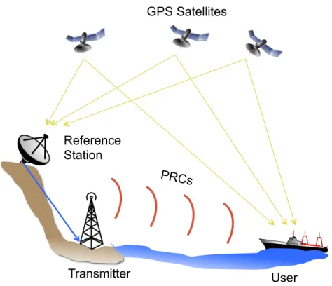
The U.S. Coast Guard is a user, developer, and supplier of a variety of maritime radio-navigation systems, including Differential Global Positioning System (DGPS). In brief, DGPS provides correction information to the user so as to improve the accuracy of GPS measurements. Pseudorange corrections for the GPS L1 coarse acquisition (C/A) signals are computed for each satellite at a reference site, and then broadcast in the nearby geographic area at each beacon’s assigned radio frequency (between 285 kHz and 325 kHz, with 500 Hz width) using minimum-shift keying (MSK) modulation at 100 bit·s−1 or 200 bit·s−1. Messages are encoded with the RTCM SC-104 standard [4, 5]. Fig. 1.1 is a diagram of typical DGPS operation in the United States.
For user safety, these DGPS corrections must be both reliably transmitted and accurate. In recent years, expansion to a greater number of beacons in the Nationwide DGPS (NDGPS) network has increased DGPS coverage, with the intent of reaching a stated goal of 99% coverage of the continental United States. Now, in most areas of the United States and its surrounding maritime waterways, at least two overlapping beacons are “visible” to littoral DGPS users—in many areas, three or more beacons are visible. A map detailing the number of beacons covering the continental United States is shown in Fig. 1.2. In typical implementations, DGPS receivers apply the corrections from the “strongest” beacon—the beacon with the highest signal-to-noise ratio (SNR) received at the user’s location.
The availability of additional information from multiple beacons raises the possibil-ity of combining (also termed “networking” in this thesis) the corrections to increase both system robustness and the accuracy of the resulting position solutions. This thesis pro-poses and evaluates various methods for networking DGPS corrections with comparison against the current method.
The DGPS radio-navigation system maintained by the U.S. Coast Guard is critical to the U.S. economy and national security, assuring reliable and accurate positioning ca-pability. Eighty-six DGPS stations throughout the country broadcast signals containing
GPS Satellites
Reference Station
Transmitter User
PRCs
Figure 1.1: Typical DGPS implementation. The reference station receives and calculates pseudoranges to visible GPS satellites, then determines the error in each satellite’s pseu-dorange by comparison to the reference site’s surveyed position. The error corrections (pseudorange corrections, or PRCs) are then broadcast from the transmitter to the user, who adds the PRCs to his own calculated pseudoranges.
tronic navigation signal, LORAN-C, was terminated in 2010, leaving the North American continent with only GPS-based navigation systems [7]. Because a loss of the position-ing accuracy provided by DGPS is hazardous to navigation, ensurposition-ing robustness and accuracy of the signal is important to both the Coast Guard and the user base.
Figure 1.2: Coverage map of the continental U.S.A. displaying number of DGPS beacons available (assuming signal strength greater than 37.5 dB·µV·m−1). Note the typical presence of three or more beacons along the three coasts, Mississippi River, and Great Lakes areas. Coverage area signal strengths were calculated using Millington’s model [8].
1.3 Impetus for current work
Networking DGPS broadcasts has the potential to improve both position accuracy and system robustness over the current DGPS solution method. Previous work indicates that positions corrected with a DGPS beacon display a bias away from the beacon used, which increases in magnitude and variation as the user travels farther from the beacon [9]. This research shows that a user’s mean position and 95% scatter radius (the radius from the mean bias containing 95% of the user’s positions1) are nearly linearly propor-tional to the user’s distance from the beacon, representative of spatial decorrelation for DGPS-corrected GPS positions [9]. Figs. 1.3(a) and 1.3(b) show the bias and scatter
radius decorrelation, respectively. Currently, a modern DGPS receiver collects and adds the pseudorange corrections from a single beacon to its calculated GPS satellite pseu-doranges. Typically, the beacon with the highest signal-to-noise ratio is selected as the beacon to use, which may or may not be the beacon closest to the user [10]. Some DGPS receivers offer the user options as to the beacon selection algorithm, with typical choices including “highest SNR”, “closest beacon”, and “manual selection”. Typical SNR is calculated from the ratio of beacon signal strength and expressed in decibels relative to atmospheric noise level.
While single-beacon solutions currently meet U.S. Coast Guard positioning
specifi-cations (ten meters 2drms everywhere, and three meters 2drms in critical waterways
[4]), why not take advantage of all the available correction information? Knowing there is an inherent bias in the user’s position because all users employ a single-beacon correction method necessitates evaluation of a better positioning algorithm [9, 11, 12]. Ionospheric SED events have been shown to cause disruptions to wide areas of DGPS service [13, 14], again raising the question: if it’s possible that the user’s primary beacon is compromised, why not use the information from a wider area of beacon coverage? Because a user’s receiver can potentially collect information from two or more DGPS beacons, it is very likely that the use of information from multiple beacons can improve the DGPS user’s position accuracy. Users become more confident that their navigation systems are oper-ating properly if they know that the receivers are applying correction information from more than just one beacon. That confidence comes from the systems potentially mit-igating sources of error (such as thermal noise, SED effects, and latency error) while simultaneously increasing position accuracy.
−6 −4 −2 0 2 4 6 −6 −4 −2 0 2 4 6 East Error (m) North Error (m) GPS DGPS (a) 0 100 200 300 400 500 600 700 800 900 1000 0 1 2 3 4 5 6 7 8 9 10
Distance from beacon (km)
95% scatter radius (m)
DGPS slope = 0.25 m/100km
GPS DGPS
(b)
Figure 1.3: (a) Typical DGPS-corrected GPS position plot for a user, showing a charac-teristic bias away from the beacon in use. (b) Comparison of DGPS and GPS position 95% scatter radii vs. distance from Saginaw Bay DGPS station (applied to CORS data), showing spatial decorrelation in the form of an increase in 95% scatter radius as the users distance to the beacon increases. Both plots reprinted with permission from [11].
1.4 Discussion of related work
Certain aspects of networked DGPS have been previously examined by a number of authors: discussion of enhanced beacon availability in Europe; existing and novel methods of beacon selection; sources of beacon errors; and several methods of networking DGPS. Below is a brief discussion of those research efforts pertinent to the topic of networking multi-beacon DGPS.
Grant considers various methods for choosing amongst multiple Differential Global Navigation Satellite System (DGNSS) beacons [10]. He considers two obvious methods: choose the nearest beacon by distance to user or the strongest beacon measured by SNR using atmospheric noise only. He also proposes including two other noise sources in the strongest beacon category: a comparison of self to skywave and signals from other beacons. In addition to existing integrity measures, Grant proposes adding time-to-alarm, recognizing that weak stations have latency in data between time-of-arrival, subsequent calculation of DGPS corrections, and broadcast time to user. Grant’s work
introduces new sources of error and emphasizes the strategy for selecting appropriate beacons to maximize algorithm productivity.
The research of Last et al. into Europe’s DGNSS examines the value of DGNSS
PRC interpolation and whether this would cause problems for the user [15]. The clock bias question arises from the difference between user and GPS satellite time, which is usually resolved by calculating this difference during locking to the frequency and phase difference. With DGNSS, there is another latency introduced by the time-to-calculation of the reference station, which is typically not of concern since all the latencies introduced by a single station are the same. During their test, the authors assessed the quantity of multi-beacon coverage areas in the United Kingdom, where three beacons was common and seven beacons was the maximum—interestingly, the maximum on the European mainland was 23! Testing consisted of using four DGNSS receivers to record transmissions and an Ashtech receiver locally-placed for actual values, which were recorded for 24 hours. They discovered that the effect of merging different clock biases was minimized due to the averaging and weighting process when combining the PRCs, and therefore was negligible. The combination method weighted the inverse of the user-beacon ranges, resulting in an improvement in correlation between calculated PRC and actual PRC (termed Regional Area Augmentation System, RAAS). Also compared were the solutions computed using single-beacon (23 km away) and RAAS (219, 358, and 419 km away) methods. They find that the single-beacon position solutions are better, but only slightly, suggesting that RAAS solutions might be useful. Their work also suggests that further work should explore a combination of two beacons, and that a RAAS could extend the boundaries of the current DGNSS system.
List of References
[1] Navstar GPS Space Segment/Navigation User Segment Interfaces, Global Position-ing Systems Directorate Specification IS-GPS-200, Rev. F, Sept. 2011.
[2] Global Positioning System Standard Positioning Service Performance Standard, Global Positioning Systems Directorate Specification GPS SPS PS, Sept. 2008.
[3] K. Borre, D. M. Akos, N. Bertelsen, P. Rinder, and S. H. Jensen,A Software-Defined GPS and Galileo Receiver: a Single-Frequency Approach. Boston, MA: Birkh¨auser, 2007.
[4] Differential Global Positioning System Broadcast Standard, United States Coast Guard Manual COMDTINST M16 577.1, Apr. 1993.
[5] RTCM Recommended Standards for Differential Navstar GPS Service, Radio Tech-nical Commission for Maritime Services (RTCM) Special Committee No. 104 Stan-dard 2.1, Jan. 1994.
[6] United States Coast Guard Navigation Center. “NDGPS general information.” [Accessed: 10 Jan. 2013]. Jan. 2013. [Online]. Available: http://www.navcen.uscg. gov/?pageName=dgpsMain
[7] “Record of Decision (ROD) on the U.S. Coast Guard Long Range Aids to Navigation (Loran-C) Program,” Federal Register, vol. 75, no. 4, pp. 997–998, Jan. 2010. [8] G. Millington, “Ground-wave propagation over an inhomogeneous smooth earth,”
in Proc. IEE—Part III: Radio and Commun. Eng., vol. 96, Jan. 1949, pp. 53–64, doi:10.1049/pi-3.1949.0013.
[9] G. W. Johnson, C. Oates, M. Wiggins, P. F. Swaszek, A. T. Page, R. J. Hartnett, and A. B. Cleveland, “USCG NDGPS accuracy and spatial decorrelation assess-ment,” inProc. 2012 Global Navigation Satellite Syst. Inst. Navigation (ION GNSS 2012), San Diego, CA, Sept. 2012, pp. 3665–3674.
[10] A. J. Grant, “Availability, continuity, and selection of maritime DGNSS radiobea-cons,” Ph.D. dissertation, Sch. Informatics, Univ. Wales, Bangor, United Kingdom, 2002.
[11] G. W. Johnson, P. F. Swaszek, and R. J. Hartnett, “Performance assessment of the
recent NDGPS recap—initial simulation results,” in Proc. 2012 Int. Tech. Meeting
Inst. Navigation (ION ITM 2012), Newport Beach, CA, Jan. 2012, pp. 1369–1376. [12] L. Sj¨oberg, G. Hedling, and A. Tiwari, “A wide area solution that takes advantage of the existing radio broadcast and national geodetic network infrastructure,” inIEEE Position Location Navigation Symp. (IEEE PLANS 1996), Atlanta, GA, Apr. 1996, pp. 596–603, doi:10.1109/PLANS.1996.509133.
[13] S. Skone and A. Coster, “Performance evaluation of DGPS versus SBAS/WADGPS for marine users,” in Proc. 20th Int. Tech. Meeting Satellite Division Inst. Naviga-tion (ION GNSS 2007), Fort Worth, TX, Sept. 2007, pp. 1904–1913.
[14] S. Skone, R. Yousuf, and A. Coster, “Combating the perfect storm: improving
marine Differential GPS accuracy with a wide-area network,” GPS World, pp. 31–
38, Oct. 2004.
[15] D. Last, A. Grant, A. Williams, and N. Ward, “Enhanced accuracy by regional operation of Europe’s new radiobeacon differential system,” inProc. 15th Int. Tech. Meeting Satellite Division Inst. Navigation (ION GPS 2002), Portland, OR, Sept.
CHAPTER 2
Networked DGPS Methods
2.1 Background
We considered various methods of networking DGPS, both previously proposed and novel, for inclusion into this research. The main criterion for evaluation was the ready availability of information to a typical user: namely, could a considered algorithm be easily employed on existing equipment? Candidate algorithms should be mathemati-cally simple to perform and dependent only on the data broadcast through the existing DGPS. These two requirements ensure that the algorithm is capable of deployment on low-cost hardware and does not require any further changes to infrastructure for the user and or the DGPS provider. In the case of this research, only DGPS within the United States is considered. While Mueller’s minimum-variance algorithm showed promising performance, it was excluded from this research because station-specific beacon charac-terization data are not available [1].
2.2 Pseudorange calculation and correction
DGPS-corrected pseudoranges are calculated by the simple subtraction of the cor-rection to the calculated pseudoranges.
˚ρs = c (δtr−δrcv) (2.1)
ˆ
ρs =ρs−c (δtr−δrcv) (2.2)
=ρs−˚ρs (2.3)
where ˚ρs is introduced as the PRC for satellite s, ρs denotes the true range
to satellite; ˆρs denotes the calculated pseudorange; c denotes the speed of light
(2.997 924 58·108m·s−1); and δ
tr −δrcv denotes the difference between the transmit-ted and received times (s) introduced by the combination of a number of errors. The sources and description of these errors are discussed further in Chapter 4.
2.3 Networking algorithms
Two categories of combining DGPS beacon PRCs are considered: (1) to weight the PRCs using some criteria and (2) to recalculate the PRC based on a beacon grouping’s spatial orientation to the user. The first category includes three algorithms, each using different criteria to weight each available satellite’s PRC, where the PRC is weighted as such: ˚ρs = B X b=1 ab˚ρb,s (2.4)
wheresdenotes the target satellite,ab is the weightaapplied to beacon b, andB is the
total number of beacons available.
2.3.1 Simple averaging
The first DGPS networking algorithm considered is an average of the available beacons. In particular, the pseudorange corrections are weighted equally and a single PRC is applied to the satellite at that time. This weighting is described as:
ab =
1
B (2.5)
where B, again, is the available number of beacons. This algorithm is proposed with
the assumption that a region of tightly-spaced beacons will broadcast relatively similar pseudorange corrections and this method might serve as a simple way to remove small perturbations between the beacons’ PRCs.
2.3.2 Inverse-range
The second DGPS networking algorithm considered is based on weighting the PRCs by the inverse of the range from the user to the beacon. This method of combining multiple beacons was first proposed by Last et al. in [2], with the intent of minimizing the effect of beacons distant from the user’s position. The user’s position may, in this
case, be established a priori via a raw GPS fix, since the distances in question are
comparison. The weights for the inverse-range method are calculated as: ab = 1 rb B X k=1 1 rb !−1 (2.6) where rb is the range from the user to beacon b, and the second term normalizes the
weights.
2.3.3 Inverse-range-squared
The third DGPS networking algorithm considered is based on weighting the PRCs by the inverse of the range-squared from the user to the beacon. We propose this new method in order to further reduce the effects of long-distance beacons on the user’s position. Particularly, since it is known that a user in close proximity to a beacon (less than about 50 km) will have a small bias length and scatter radius when applying a single DGPS beacon’s corrections that particular beacon’s weight should, therefore, dominate within both range-based algorithms [3]. As with the inverse-range method, the user’s position is establisheda priori with a GPS fix. The weights for the inverse-range-squared algorithm are calculated as:
ab = 1 r2b B X k=1 1 r2b !−1 (2.7) where the variables are represented in the same manner as the inverse-range method.
2.3.4 Spatial linear interpolation (SLI)
The fourth and final DGPS networking algorithm considered is based on fitting a hyperplane to the known locations and distances of the beacons relative to the user’s location. In the case of three beacons, this method describes linear interpolation between three points and the user’s general location. We propose this new method because it takes into account the spatial geometry and orientation of the beacon grouping (i.e.: ranges and azimuths to the beacons) relative to the user, which, as described previously, are a factor in DGPS-user position bias. Because the precise locations of all the U.S. DGPS beacons are known, this information may be stored so the user may apply received
the grid as the x, y coordinates and the PRCs assume the z values. The three points that are created form the basis of an SLI hyperplane, which is evaluated at the user’s assumed location (which, again, may be provided through a rough GPS fix). The SLI algorithm is described by:
˚ ρs=ax+by+c pR (2.8) pb = DDNE ˚ ρb,s (2.9)
where x and y denote the grid coordinates, akin to longitude and latitude, a, b, and c
describe the coefficients of the equation of the plane (note: this a is unrelated to the weighting coefficient, ai) through the three beacon-PRC points (pb), pR is the position vector of the rover (the user)—by convention here, the point (0, 0), andDN andDEare the great circle distances North and East of the user. The plane equation coefficients,a,
b, and care given by:
∆ =x1(y2−y3)−x2(y1−y3) +x3(y1−y2) (2.10) a= (−∆)−1 (z1−z2)(x1−x3)−(z1−z3)(x1−x2) (2.11) b= (+∆)−1 (z1−z2)(y1−y3)−(z1−z3)(y1−y2) (2.12) c=z1−ax1−by1 (2.13)
Spatial linear interpolation computational methods
Because the area of interest is linearized inx,y and z, the pseudorange correction may be calculated directly with either vector or linear algebra. Selection of an appropri-ate computation method is dependent on the requirements of the user and may depend on computing capabilities.
Vector method
This method calculates the user’s PRC by manipulating the position-PRC vectors at each beacon described in (2.9):
n= (p1−p3)×(p2−p3) (2.14) p0 =−p⊤3 (p1×p2) (2.15) ˚ ρs=− p0 nz (2.16) where n is the vector normal to the plane, (×) is the cross product of two vectors, p0 is the pseudorange correction at a point on the plane at (0,0), p1 through p3 represent the 3-dimensional position-PRC vectors of the beacons, relative to the user position at (0,0), andnz represents the zcomponent of the normal vector.
Linear algebra method
This method calculates the user’s PRC by rearranging the plane equation such that it satisfies a set of simultaneous linear equations, then solved at the user’s location:
z1 z2 z3 | {z } z = ax1+by1+c ax2+by2+c ax3+by3+c = x1+y1+ 1 x2+y2+ 1 x3+y3+ 1 | {z } A a b c |{z} c (2.17) c=A−1z (2.18) ˚ρs =x⊤z x⊤=[0,0,1] (2.19) whereAis non-singular and represents the beaconx, y position matrix,crepresents the vector containing the coefficients of the plane equation [a, b, c]⊤,z represents the vector containing the pseudorange correction values, andx represents the user’s position-PRC vector at the origin.
Weighting coefficients
So as to conform to the convention of (2.4), the coefficients of the SLI algorithm may be obtained by rearranging the algebraic forms of the equation of the plane, (2.11) to (2.13), such that the PRC weighting coefficients, ai, correspond to their respective
a1= ∆−1 (y2−y3)−(x2−x3) + (x2y3−x3y2) (2.20) a2= ∆−1 (y1−y3) + (x1−x3)−(x1y3−x3y1) (2.21) a3= ∆−1 (y1−y2)−(x1−x2) + (x1y2−x2y1) (2.22) List of References
[1] T. Mueller, “Minimum variance network DGPS algorithm,” inIEEE Position
Loca-tion NavigaLoca-tion Symp. (IEEE PLANS 1994), Las Vegas, NV, Apr. 1994, pp. 418–425, doi:10.1109/PLANS.1994.303344.
[2] D. Last, A. Grant, A. Williams, and N. Ward, “Enhanced accuracy by regional operation of Europe’s new radiobeacon differential system,” inProc. 15th Int. Tech. Meeting Satellite Division Inst. Navigation (ION GPS 2002), Portland, OR, Sept. 2002, pp. 2723–2732.
[3] G. W. Johnson, P. F. Swaszek, and R. J. Hartnett, “Performance assessment of the
recent NDGPS recap—initial simulation results,” in Proc. 2012 Int. Tech. Meeting
CHAPTER 3
Simulating Networked DGPS
3.1 Applicable software
We performed the simulator testing on a Spirent GSS8000 GNSS simulator, which was governed by the SimGEN software package. Data were logged in SimGEN and
post-processed in theMatlabenvironment, using L3NAV Systems’ GPS toolbox. We replace
the word “user” with a new term “rover” when discussing a simulated vehicle’s position, so as to clearly differentiate between the simulator vehicle and the real-life equipment user.
3.2 Simulator testing overview
We tested the effectiveness of the various networked DGPS algorithms was per-formed on a Spirent GSS8000 simulator. This GNSS simulator provided a reliable and verbose output log of the settings and states of the variables-of-interest, such as distinct satellite ranges, pseudoranges, ionospheric and tropospheric offsets. Because southeast-ern New England contains good multi-beacon coverage (sufficient quantity and spatial variety of DGPS beacons) and a balanced mix of land and water that forms the en-trance to New York harbor, we chose this area for the testing region. We configured the simulator to best compare the networking algorithms against each other; in this vein, the simulator was set to produce only ionospheric and tropospheric delays. Ionospheric effects were generated using the Klobuchar model; tropospheric effects were generated using the NATO STANAG 4294 model. The surface refractivity index was set to the recommended value of 324.8 [1]. Error modeling with thermal and spurious noise sources is outside the scope of this thesis and is part of future work. Receiver-GPS clock bias was turned off, and the rover maintained a static position for the duration of each test. All simulations used the World Geodetic System 1984 geodetic reference ellipsoid (WGS84) and rover reference positions of 0 m altitude for the sake of simplicity.
0 100 200 300 400 0 100 200 300 400 2.05 2.1 2.15 2.2 2.25 2.3 2.35 2.4 Distance East (km) Distance North (km)
Atmospheric correction (sec
×
1
⋅
10
−8)
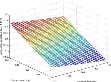
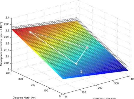
Figure 3.1: Total atmospheric correction (ionospheric + tropospheric error terms) for SV 22 observed across 400 km by 400 km area over New England during GNSS simulation. This is referenced in this thesis as the “actual PRC” plot.
First, the simulator was used to produce a representation of the atmospheric offsets at a single time, across the New England region. The New England area tested was a grid originating with its southwest point at 40.0°N, 74.5°W (approximately Joint Base McGuire-Dix-Lakehurst, located in northeast New Jersey) and advancing approximately 400 km north and east. The area chosen encompassed the DGPS beacons of interest, with the intent of determining the appearance and behavior of the atmospheric corrections over a geographic area. Data points were collected every 10 km north and east from the origin for the same time. This representation provides a baseline for comparing the suitability of each networking algorithm. Fig. 3.1 shows the grid and contours of the simulation for a single satellite; of particular note is the near-planar behavior over the region of interest.
The second simulator test plotted the position solutions calculated by the networking algorithms over a 24-hour period and specific DGPS beacon groups. Two beacon groups were selected to be “visible” to the rover on the basis of their spatial geometries. Group
77° W 76° W 75° W 74° W 73° W 72° W 71° W 70° W 69° W 39° N 40° N 41° N 42° N 43° N 44° N Group 1 Group 2 Acushnet, MA Hudson Falls, NY Sandy Hook, NJ Moriches, NY A B C D E F
Figure 3.2: Map of simulator testing locations (red diamonds) and DGPS beacons (blue triangles), with beacon groups labeled. Lambert projection.
1 was intended to represent the region’s actual atmospheric effects most accurately, and was comprised of a widely-spaced beacon group including Acushnet, MA; Hudson Falls, NY; and Moriches, NY. The Group 1 beacon geometry could be considered as “optimal” to a user because it is well-spaced geographically. Group 2 was intended to be a “realistic” set of beacons that might be typically visible to a marine user, comprised of a nearly-linear beacon group including Acushnet, MA; Moriches, NY; and Sandy Hook, NJ. Rover positions were labeled “A” through “F”, and were chosen to place the rover and beacons in unique and interesting configurations, such as: “optimal”—rover in the center of the beacon triangle, rover between two beacons, and rover outside the beacon triangle. Fig. 3.2 indicates the beacon positions, beacon group outlines, and rover static positions used during testing.
In addition to the group-point test locations, an “operational” test was performed intended to replicate the kind of transit through Long Island Sound (LIS) that a mariner might undertake. This test is also designed to showcase the performance of the
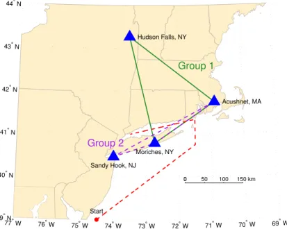
69° W 39° N 40° N 41° N 42° N 43° N 44° N 77° W 76° W 75° W 74° W 73° W 72° W 71° W 70° W Group 1 Group 2 Acushnet, MA Hudson Falls, NY Sandy Hook, NJ Moriches, NY Start 0 50 100 150 km 0
Figure 3.3: Map of a mariner’s Long Island Sound transit, as an operational test, on the simulator. Lambert projection.
ing algorithms as the rover passes through a variety of distances, azimuths, and spatial orientation vectors from the beacon groupings. Fig. 3.3 shows this transit.
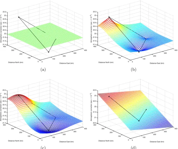
In order to understand the behavior of each networking algorithm, visualizations were generated using the Group 1 beacon set and the same geographic region and similar time window represented in Fig. 3.1. Fig. 3.4 shows the beacon grouping and associated PRCs overlaid on the PRC solution for each networking algorithm. Fig. 3.5 shows the SLI algorithm’s behavior overlaid on the “actual PRC” plot from Fig. 3.1 (in gray mesh), as well as rover position D, demonstrating how the SLI hyperplane is extrapolated to the rover’s position. Here, a 100 ms time difference is introduced so that the difference between the “actual PRC” grid and the SLI hyperplane may be observed more clearly as a slight vertical offset between the two.
0 100 200 300 400 0 100 200 300 400 21.4 21.6 21.8 22 22.2 22.4 22.6 22.8 23 23.2 Distance East (km) Distance North (km)
Atmospheric correction (sec
× 1 ⋅ 10 −9) (a) 0 100 200 300 400 0 100 200 300 400 21.4 21.6 21.8 22 22.2 22.4 22.6 22.8 23 23.2 Distance East (km) Distance North (km)
Atmospheric correction (sec
× 1 ⋅ 10 −9) (b) . 0 100 200 300 400 0 100 200 300 400 21.4 21.6 21.8 22 22.2 22.4 22.6 22.8 23 23.2 Distance East (km) Distance North (km)
Atmospheric correction (sec
× 1 ⋅ 10 −9) (c) 0 100 200 300 400 0 100 200 300 400 20.5 21 21.5 22 22.5 23 23.5 Distance East (km) Distance North (km)
Atmospheric correction (sec
× 1 ⋅ 10 −9) (d)
Figure 3.4: Representations of the networking methods, plotted with respect to the area covered by Fig. 3.2 and Group 1 beacons: (a) simple-averaging, (b) inverse-range, (c) inverse-range-squared, (d) spatial linear interpolation.
0 100 200 300 400 0 100 200 300 400 2 2.05 2.1 2.15 2.2 2.25 2.3 2.35 2.4 Distance East (km) Distance North (km)
Atmospheric correction (sec
×
1
⋅
10
−8)
Figure 3.5: Representation of SLI’s hyperplane (colored) overlaid on the “actual PRC” plot from Fig. 3.1 (gray grid), with DGPS beacon triangle and rover position D plotted in white on the SLI hyperplane.
3.3 Simulator testing results
When evaluating performance, the networking algorithms should be compared against each other and then again to single-beacon position solutions. Of particular interest are three values: (1) the time-averaged position bias length; (2) the radius con-taining 95% of the position solutions from the bias length, termed the scatter radius; and (3) the 2×distance-root-mean-squared (2drms) value for each method’s 2-dimensional
position solutions. The bias length is the distance between the mean position solution and the true position. The scatter radius, with respect to the bias length, helps de-termine the precision of the solution method. Note: this is not the commonly-known R95 measure, which describes the radius including 95% of positions with respect to true
position. The third measure of performance, 2drms, describes a common measure of
horizontal accuracy (m), referencing both true position and position precision, given by:
2drms= 2 q
σ2
x+σy2 (3.1)
whereσx and σy (m) are the standard deviations of thex and yposition values,
respec-tively.
The positions for the DGPS beacon groups and rover locations are plotted in Figs. 3.6 through 3.14. Also plotted are the time-averaged bias lengths, denoted with a large dot placed at the center of mass of positions, the 95% radius (denoted with a dotted circle, and the true position (0, 0) point overlaid with thick black crosshairs.
−3 −2 −1 0 1 2 3 −3 −2 −1 0 1 2 3
East position error, in meters
North position error, in meters
Acushnet, MA Hudson Falls, NY Moriches, NY (a) Single-beacon. −3 −2 −1 0 1 2 3 −3 −2 −1 0 1 2 3
East position error, in meters
North position error, in meters
Averaging 1/Range 1/Range2 SLI
(b) Networked beacons. Figure 3.6: Simulator position plots for Beacon Group 1, Rover Position A.
−3 −2 −1 0 1 2 3 −3 −2 −1 0 1 2 3
East position error, in meters
North position error, in meters
Acushnet, MA Hudson Falls, NY Moriches, NY (a) Single-beacon. −3 −2 −1 0 1 2 3 −3 −2 −1 0 1 2 3
East position error, in meters
North position error, in meters
Averaging 1/Range 1/Range2 SLI
(b) Networked beacons. Figure 3.7: Simulator position plots for Beacon Group 1, Rover Position B.
−3 −2 −1 0 1 2 3 −3 −2 −1 0 1 2 3
East position error, in meters
North position error, in meters
Acushnet, MA Hudson Falls, NY Moriches, NY (a) Single-beacon. −3 −2 −1 0 1 2 3 −3 −2 −1 0 1 2 3
East position error, in meters
North position error, in meters
Averaging 1/Range 1/Range2 SLI
(b) Networked beacons. Figure 3.8: Simulator position plots for Beacon Group 1, Rover Position C.
−3 −2 −1 0 1 2 3 −3 −2 −1 0 1 2 3
East position error, in meters
North position error, in meters
Acushnet, MA Hudson Falls, NY Moriches, NY (a) Single-beacon. −3 −2 −1 0 1 2 3 −3 −2 −1 0 1 2 3
East position error, in meters
North position error, in meters
Averaging 1/Range 1/Range2 SLI
(b) Networked beacons. Figure 3.9: Simulator position plots for Beacon Group 1, Rover Position D.
−3 −2 −1 0 1 2 3 −3 −2 −1 0 1 2 3
East position error, in meters
North position error, in meters
Acushnet, MA Hudson Falls, NY Moriches, NY (a) Single-beacon. −3 −2 −1 0 1 2 3 −3 −2 −1 0 1 2 3
East position error, in meters
North position error, in meters
Averaging 1/Range 1/Range2 SLI
(b) Networked beacons. Figure 3.10: Simulator position plots for Beacon Group 1, Rover Position E.
−3 −2 −1 0 1 2 3 −3 −2 −1 0 1 2 3
East position error, in meters
North position error, in meters
Acushnet, MA Hudson Falls, NY Moriches, NY (a) Single-beacon. −3 −2 −1 0 1 2 3 −3 −2 −1 0 1 2 3
East position error, in meters
North position error, in meters
Averaging 1/Range 1/Range2 SLI
(b) Networked beacons.
Figure 3.11: Simulator position plots for Beacon Group 1, Rover Transit through Long Island Sound.
−3 −2 −1 0 1 2 3 −3 −2 −1 0 1 2 3
East position error, in meters
North position error, in meters
Acushnet, MA Sandy Hook, NJ Moriches, NY (a) Single-beacon. −3 −2 −1 0 1 2 3 −3 −2 −1 0 1 2 3
East position error, in meters
North position error, in meters
Averaging 1/Range 1/Range2 SLI
(b) Networked beacons. Figure 3.12: Simulator position plots for Beacon Group 2, Rover Position D.
−3 −2 −1 0 1 2 3 −3 −2 −1 0 1 2 3
East position error, in meters
North position error, in meters
Acushnet, MA Sandy Hook, NJ Moriches, NY (a) Single-beacon. −3 −2 −1 0 1 2 3 −3 −2 −1 0 1 2 3
East position error, in meters
North position error, in meters
Averaging 1/Range 1/Range2 SLI
(b) Networked beacons. Figure 3.13: Simulator position plots for Beacon Group 2, Rover Position E.
−3 −2 −1 0 1 2 3 −3 −2 −1 0 1 2 3
East position error, in meters
North position error, in meters
Acushnet, MA Sandy Hook, NJ Moriches, NY (a) Single-beacon. −3 −2 −1 0 1 2 3 −3 −2 −1 0 1 2 3
East position error, in meters
North position error, in meters
Averaging 1/Range 1/Range2 SLI
(b) Networked beacons. Figure 3.14: Simulator position plots for Beacon Group 2, Rover Position F.
−3 −2 −1 0 1 2 3 −3 −2 −1 0 1 2 3
East position error, in meters
North position error, in meters
Acushnet, MA Sandy Hook, NJ Moriches, NY (a) Single-beacon. −3 −2 −1 0 1 2 3 −3 −2 −1 0 1 2 3
East position error, in meters
North position error, in meters
Averaging 1/Range 1/Range2 SLI
(b) Networked beacons.
Figure 3.15: Simulator position plots for Beacon Group 2, Rover Transit through Long Island Sound.
3.4 Discussion of simulator results
Fig. 3.16 demonstrates the performance metrics for each of the single-beacon and networked-beacon algorithms, categorized by Group-Point. As expected, the position solutions using corrections from a single DGPS beacon exhibit a bias away from the bea-con. This is evident in every test case, with the magnitude of the bias being proportional to the distance away from the beacon. The azimuth of the bias remains constant, as expected. The 95% scatter radii magnitudes are also proportional to the distance away from the beacon. 2drmsvalues suffer for those beacons that are far away from the rover.
These results corroborate the results from previous work on DGPS bias.
Position solutions generated from networked-beacon algorithms tend to be better than those generated from single-beacon solutions in terms of all three performance
metrics. In unique cases where the rover is very close to a beacon (within ∼50 km),
however, single-beacon solutions perform very similarly to networked-beacon solutions. Among the four networked-beacon algorithms, the simple-averaging method shows the greatest average values of bias length, scatter radius, and 2drms in all cases. We
expect this because the simple-averaging method does not take into account the rover’s position relative to the beacon, nor the beacon group geometries—it simply accounts for differences in beacon PRCs, which may be useful in an especially noisy environment or when the beacons are very close together. This method exhibits a very obvious bias away from the beacons, only mitigated when the rover is located equidistant to and in the center of all three beacons (see Group 1 Point A, denoted “1A”). As can be surmised, this
method’s 2drms values approximate an average among the three single-beacon2drms
values.
In all three metrics, the inverse-range and inverse-range-squared methods performed as well or better than the simple-averaging method. Again, this is to be expected, as these methods de-weight the beacons farther away and thus remove the greater biases (both length and scatter radius) from the position solutions. Consequently, the 2drmsvalues
squared method than for the simple inverse-range because the squaring exponent places a greater emphasis on the closest beacon, even when all three are approximately the same distance from the rover (see position plot for Group 2 Point E). However, in all cases, these two methods exhibit a definite bias away from the beacons, caused by the algorithms’ indifference to the beacon geometry. Because of the use of range, these methods are more precise than the simple-averaging method, and retain a slight bias.
The spatial linear interpolation method performs uniquely when compared against both single-beacon and other networked-beacon networking methods. In all cases, the bias length value for this method is smaller than for all other solution methods and the
2drmsvalue is almost always the smallest. In any case, the2drmsvalues are significantly
lower than almost all single-beacon solutions. This is particularly expected due to the calculated SLI hyperplane closely approximates the near-planar “actual” atmospheric correction grid from the first simulator test. However, the 95% scatter radius exhibits interesting properties when the beacon geometry is nearly linear and the rover is located at a tangent to the beacon line. In this case, the SLI solution is accurate, but with
a greater scatter radius, and a 2drms value lower than all other solutions. In that
peculiar arrangement, SLI’s large scatter radius is caused by the orientation of the GPS constellation to the beacon group: as the satellites rise and fall, they come into and disappear from each beacon’s view at different times. Because GPS position calculations require at least four satellites and, during this time, this may not be the case, the SLI correction may be, briefly, based entirely on a single satellite, and the position solutions behave with the bias of a single-beacon solution. A satellite count for group-point 1E, the rover-beacon orientation least likely to contain overlapping views of satellites, is shown in Fig. 3.17. However, a GPS constellation of only four visible satellites is unlikely to occur for a long time period except at high latitudes. Based on these results, the SLI
method produces, in most cases, the best2drmsperformance when compared with other
1A 1B 1C 1D 1E 1LIS 2D 2E 2F 2LIS 0 0.5 1 1.5 2 2.5 3 Group−Point Bias Length (m)
Atmos Bcn 1 Bcn 2 Bcn 3 Avg 1/R 1/R2 SLI (a) Bias length comparison.
1A 1B 1C 1D 1E 1LIS 2D 2E 2F 2LIS 0 1 2 3 4 5 6 7 8 Group−Point 95% Scatter Radius (m)
Atmos Bcn 1 Bcn 2 Bcn 3 Avg 1/R 1/R2 SLI (b) 95% scatter radius comparison.
1A 1B 1C 1D 1E 1LIS 2D 2E 2F 2LIS 0 1 2 3 4 5 6 7 Group−Point 2DRMS (m)
Atmos Bcn 1 Bcn 2 Bcn 3 Avg 1/R 1/R2 SLI (c)2drmscomparison.
Figure 3.16: Bar graphs of bias length, scatter radius containing 95% of the positions, and2drms. Bcn 1 is Acushnet, MA; Bcn 2 is Sandy Hook, NJ or Hudson Falls, NY, as
appropriate; Bcn 3 is Moriches, NY; and LIS is Long Island Sound.
2 4 6 8 10 12 14 16 18 20 22 24 0 2 4 6 8 10 12
Time Into Simulation (hours)
No. Satellites Used
Sat. Count Mean 1σ Bound
Figure 3.17: Satellite count for Point-Group 1E. The mean SV count is 9.21 and the standard deviation (1σ) is 1.81. The lowest count of usable satellites, four, was present
List of References
[1] J. P. Collins, “Assessment and development of a tropospheric delay model for air-craft users of the Global Positioning System,” M.S. thesis (Tech. Report No. 203), Dept. Geodesy, Geomatics Eng., Univ. New Brunswick, Fredericton, New Brunswick, Canada, Sept. 1999.
CHAPTER 4
Characterizing Networked DGPS Algorithm Performance
4.1 Overview
Thus far, we have introduced the concept of networking DGPS, proposed various methods of combining multiple beacons, and implemented those algorithms at various locations in New England. Because the previous chapter examined distinct points, those results are not sufficient to conclude that networked-beacon solutions offer improved per-formance over a complete DGPS coverage region. Characterizing the regional behavior of networked DGPS algorithms is necessary to accurately gauge overall performance.
We characterize algorithm behavior by examining two topics. First, we discuss the performance of each algorithm as a function of spatial orientation. We distinguish the performance of each algorithm by testing each algorithm with respect to distance and azimuth from the beacon groupings. Second, we consider each of the assumptions made up to this point. In particular, the effect of noise on performance of networked DGPS is introduced and examined.
4.2 Characterizing spatial behavior
A review of the previous chapter’s simulations shows that at each point tested, networking algorithms yield position performance improvements over single-beacon so-lutions. Moreover, the user’s position relative to the beacon grouping and the selection of the beacon grouping somehow impacts the performance of each networking algorithm. Less clear, however, is how the aforementioned factors relate to the performance of the algorithms.
In this section, we seek to characterize algorithm performance by examining the spa-tial behavior of the networking algorithms on the simulator. In particular, we evaluate
2drmsperformance relative to the spread of the beacon grouping, the beacon grouping
perfor-4.2.1 Performance versus distance
First, we evaluate algorithm performance versus distance to a beacon grouping. Beacon Group 2 is used to evaluate networked DGPS performance versus user positions located every 50 km from 0 km to 400 km due south and east of Moriches, NY. Fig. 4.1 shows the points tested, in addition to the beacon triangles’ centroids, marked with crosshairs.
The first comparison is performance versus distance south relative to the choice of
beacon grouping. Fig. 4.2 demonstrates the 2drms performance of each algorithm on
the run south, broken down by beacon grouping. In this case, the only difference between the two data sets is the choice of the third beacon: where Group 1 uses Hudson Falls, NY, and has a beacon grouping that is geographically diverse, Group 2 uses Sandy Hook, NJ, and has a linearly distributed beacon grouping oriented along a northeast axis. In this scenario, the starting point is nearly co-located with the Group 2 centroid, but is
offset from the Group 1 centroid by approximately 120 km. In both graphs, the2drms
performance degrades linearly with the user’s distance from the Moriches beacon, an effect known asspatial decorrelation. We observe the following:
1. Networked Group 1 beacons exhibit a wide variation between the linear spatial decorrelation coefficients, whereas networked Group 2 beacons exhibit similar co-efficients.
2. Averaging and range-based networked Group 1 beacons exhibit equivalent or poorer
2drmsperformance than single-beacon solutions using Moriches, NY. Group 1 SLI
performs significantly better than all other algorithms.
3. Networked Group 2 beacons offer no significant performance improvement over what is typically the closest beacon (Moriches, NY) in this direction.
4. Group 2 SLI performs slightly better than the single-beacon solution of the closest beacon. In both scenarios, the single-beacon solution with the lowest2drmsvalues
The second comparison is performance versus distance east relative to the choice
of beacon grouping. Fig. 4.3 demonstrates 2drms performance on the run east, again
broken down by beacon grouping. In this scenario, we expect that the networked Group 1 beacons will perform similar to the southerly direction and that the networked Group 2 beacons will perform better than in the southerly direction. In this test, we compare the2drmsperformance runs east and runs south for each beacon grouping.
1. Group 1 east to Group 1 south. In an easterly direction, networked Group 1 beacons performed similarly to those in the southerly direction. That is: the lines of best fit exhibit similar rates of spatial decorrelation. Only the range-based networking algorithms showed an improvement, attributable to the decreased distances from the beacons and a finding that is informative. As expected, the SLI algorithm maintained the lowest spatial decorrelation coefficients.
2. Group 2 east to Group 2 south. For Group 2 beacons in an easterly direction, the networking algorithms exhibit a much greater diversity of spatial decorrelation coefficients than in the southerly direction. Again, SLI provides the lowest2drms
values at all distances. Of note is that the2drmsperformance appears to improve
when traveling in a direction better approximating the beacon line.
3. Group 2 east to Group 1 east. The networked DGPS algorithms’ performances appear very similar to the Group 1 beacons in the easterly direction. Of interest
is that Group 2 SLI shows excellent2drmsimprovement over single-beacon up to
200 km and Group 1 SLI shows excellent improvement over single-beacon for all distances.
Table 4.1 documents the coefficients for each algorithm’s performance over distance,
assuming the performance is approximately linear. Nonlinear 2drms performance is
evident in those single-beacon solutions where the user’s azimuth to the beacon changes quickly and are noted as such in table.
char-Table 4.1: Linear coefficients of 2drmsperformance over distances south and east from
Moriches, NY, by beacon grouping. Nonlinear data is noted and excluded from compar-ison due to high azimuthal rate of change. Note that beacons 1 and 2 are not located at Moriches, NY, and exhibit an initial offset. Beacon 1 is Acushnet, MA, Beacon 2 is Hudson Falls, NY, for Group 1 and Sandy Hook, NJ, for Group 2, and Beacon 3 is Moriches, NY.
Algorithm Direction Group Coefficient Group Coefficient
(cm/100 km) (cm/100 km)
Beacon 1 South 1 67.341 2 67.341
Beacon 2 South 1 69.252 2 Nonlinear
Beacon 3 South 1 87.647 2 87.647
Average South 1 73.643 2 81.109
1/Range South 1 93.903 2 85.233
1/Range2 South 1 94.629 2 83.792
SLI South 1 33.006 2 78.051
Beacon 1 East 1 Nonlinear 2 67.341
Beacon 2 East 1 Nonlinear 2 81.134
Beacon 3 East 1 87.785 2 87.785
Average East 1 Nonlinear 2 80.183
1/Range East 1 74.691 2 75.814
1/Range2 East 1 69.240 2 67.839
SLI East 1 24.866 2 57.576
single-beacon DGPS solutions exhibit the same characteristic spatial decorrelation (see Chapter 1). If we combine the corrections from each DGPS beacon, we expect to re-duce the magnitude of single-beacon spatial decorrelation. We note that single-beacon algorithms using corrections from beacons farther from the user tend to have the highest
2drmsvalues. In each scenario, the averaging algorithm exhibited2drms performance
comparable to an average of the three beacons’2drmsvalues. Inverse-range and
inverse-range-squared algorithms performed better in every case than the simple averaging. The SLI algorithm had the lowest2drmsvalues of all the algorithms, and was bounded from
higher2drmsvalues by the best-performing single-beacon solutions. Note that the SLI
solution’s 2drms performance is highly dependent on the beacon geometry and the
di-rection of travel relative to the beacon grouping’s axis. We examine this aspect is further in the next section.
76° W 74° W 72° W 70° W 68° W 38° N 40° N 42° N Group 1 Group 2 Acushnet, MA Hudson Falls, NY Moriches, NY Sandy Hook, NJ 00 50 100 150 km Run S Run E
Figure 4.1: 2drms performance testing locations due south and east of Moriches, NY.
0 50 100 150 200 250 300 350 400 0 1 2 3 4 5 6
Distance from Moriches, NY (km)
2DRMS (m) Acushnet, MA Hudson Falls, NY Moriches, NY Averaging 1/Range 1/Range2 SLI
(a) Using Group 1 beacons.
0 50 100 150 200 250 300 350 400 0 1 2 3 4 5 6
Distance from Moriches, NY (km)
2DRMS (m) Acushnet, MA Sandy Hook, NJ Moriches, NY Averaging 1/Range 1/Range2 SLI
(b) Using Group 2 beacons.
0 50 100 150 200 250 300 350 400 0 1 2 3 4 5 6
Distance from Moriches, NY (km)
2DRMS (m) Acushnet, MA Hudson Falls, NY Moriches, NY Averaging 1/Range 1/Range2 SLI
(a) Using Group 1 beacons.
0 50 100 150 200 250 300 350 400 0 1 2 3 4 5 6
Distance from Moriches, NY (km)
2DRMS (m) Acushnet, MA Sandy Hook, NJ Moriches, NY Averaging 1/Range 1/Range2 SLI
(b) Using Group 2 beacons.
4.2.2 Performance versus azimuth
The point-group and performance versus distance tests from Chapter 3 and
Sec-tion 4.2.1 indicate that networked DGPS 2drms performance changes with the user’s
azimuth to the beacon set. We now evaluate the second performance category: net-worked DGPS performance versus the user’s azimuth to the beacon grouping. Each beacon grouping was tested at locations every 30° from the grouping’s centroid at vari-ous radii. Beacon grouping 2 was tested at Moriches, NY, because it is approximately co-located with the centroid. Beacon grouping 1 was tested at radii of 200 km and 400 km, and Group 2 was tested at radii of 100 km and 200 km. Figs. 4.4 and 4.6 indicate the ge-ographic locations of the test radials, and include the beacon triangles’ centroids marked with crosshairs.
The first scenario considers2drmsperformance versus azimuth relative to the Group
1 centroid. This establishes a baseline of2drmsperformance by using a spatially diverse
beacon grouping. Figs. 4.5(a) and 4.5(b) plot the2drmsperformance versus azimuth at
radii of 200 km and 400 km, respectively. The networked algorithms have 2drmsvalues
that are lower than the single-beacon solutions for both radial distances in this scenario. At both distances, the SLI algorithm performs significantly better at all angles than any other correction algorithm. Of interest from Figs. 4.5(a) and 4.5(b) are the following observations:
• The averaging algorithm smoothes the apparent bias directions from the
single-beacon solutions.
• The range-based algorithms exhibit the poorest2drmsperformance along a
North-east axis (angles 240° and 60°), which corresponds to the greatest sum of user distances to each beacon.
• The2drms values of SLI are nearly equal at all angles, suggesting that this
algo-rithm de-weights the proximity of the user to the nearest beacon more so than the other networking algorithms. This behavior is more evident in Fig. 4.5(b).