2006
Development of an adaptive fuzzy logic controller
for HVAC system
Rahul Laxman Navale
Iowa State UniversityFollow this and additional works at:
https://lib.dr.iastate.edu/rtd
Part of the
Mechanical Engineering Commons
This Dissertation is brought to you for free and open access by the Iowa State University Capstones, Theses and Dissertations at Iowa State University Digital Repository. It has been accepted for inclusion in Retrospective Theses and Dissertations by an authorized administrator of Iowa State University Digital Repository. For more information, please [email protected].
Recommended Citation
Navale, Rahul Laxman, "Development of an adaptive fuzzy logic controller for HVAC system " (2006).Retrospective Theses and Dissertations. 1287.
by
Rahul Laxman Navale
A thesis submitted to the graduate faculty
in partial fulfillment of the requirements for the degree of DOCTOR OF PHILOSOPHY
Major: Mechanical Engineering
Program of Study Committee: Ron M. Nelson, Major Professor
Michael Pate Greg Luecke Steve Hoff Eric Bartlett
Iowa State University Ames, Iowa
2006
INFORMATION TO USERS
The quality of this reproduction is dependent upon the quality of the copy submitted. Broken or indistinct print, colored or poor quality illustrations and photographs, print bleed-through, substandard margins, and improper alignment can adversely affect reproduction.
In the unlikely event that the author did not send a complete manuscript and there are missing pages, these will be noted. Also, if unauthorized copyright material had to be removed, a note will indicate the deletion.
UMI
UMI Microform 3217301
Copyright 2006 by ProQuest Information and Learning Company. All rights reserved. This microform edition is protected against
unauthorized copying under Title 17, United States Code.
ProQuest Information and Learning Company 300 North Zeeb Road
P.O. Box 1346 Ann Arbor, Ml 48106-1346
Graduate College Iowa State University
This is to certify that the doctoral dissertation of Rahul Laxman Navale
has met the dissertation requirements of Iowa State University
Major Professor
For the Major Program
Signature was redacted for privacy.
Table of Contents
List of Tables vii
List of Figures ix
Nomenclature xiii
List of Acronyms xvi
Acknowledgement xvii
Abstract xviii
Chapter 1 Introduction 1
1.1 Background/Literature Review 1
1.1.1 Fuzzy Logic Controllers 2
1.1.2 Summary 8
1.2 Project Objectives 8
1.3 The Adaptive FLC description 8
1.4 Proposed Adaptive Fuzzy Logic Controller - GA 9
1.5 Proposed Adaptive Fuzzy Logic Controller - ES 11
1.6 Plan of Work 12
1.7 Outline of Contents 13
Chapter 2 Experimental Facility Description 15
2.1 Introduction 15
2.2 Thermal Loads 16
2.3 Air Handling Unit 17
2.4 Cooling Plant 19
2.5 Data Acquisition 20
2.6 Bias Study for System A and System B 22
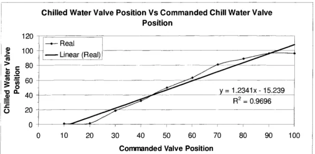
2.7 Chilled Water Valve Position Study 24
2.7.1 Introduction 24
2.7.2 Commanded and Real Chilled Water Valve Position 24
2.7.3 Chilled Water Flow Through the Cooling Coil ..26
2.8 Summary 29
Chapter 3 Performance Indices 31
3.1 Introduction 31
3.1.1 Root Mean Square Error 31
3.1.2 Controller Performance Parameters 32
3.1.3 Hydronic Energy 33
3.1.4 Actuator Travel Distance 36
3.2 Summary 37
Chapter 4 Cooling Coil Models 38
4.1 Introduction 38
4.2 Model using Neural Networks 38
4.2.1 Introduction 38
4.2.2 Normalization 39
4.2.3 Training of Neural Networks Model 41
4.2.4 Summary 42
4.3.1 Introduction 43
4.3.2 GRNN Theory 43
4.3.3 GRNN Models 45
4.3.4 Summary 47
4.4 Model using Adaptive Neural Networks 47
4.4.1 Introduction 47
4.4.2 Summary 47
4.5 Model using Lumped Capacitance Method 47
4.5.1 Introduction 47
4.5.2 Lump Capacitance Model Development 48
4.5.3 Summary 57
4.6 Summary 57
Chapter 5 Development of a Fuzzy Logic Controller 58
5.-1 Basics of Fuzzy Logic Controller 58
5.1.1 Fuzzification 58
5.1.2 Fuzzy Rule Matrix 60
5.1.3 Defuzzification Methods 60
5.2 Manual Tuning of FLC 61
5.2.1 Modifying FRM 61
5.2.2 Modifying Selective Rule in the FRM 63
5.2.3 Modifying Shape of Fuzzy Membership Functions: 64
5.2.4 Modifying Scaling Factor 65
5.3 Adaptive Fuzzy Logic Controller 66
5.3.1 Introduction 66
5.3.2 Adaptation Mechanism 67
5.3.3 Use of ES for Evolving Scaling Factor: 69
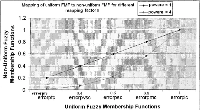
5.3.4 Use of ES for Evolving Mapping Factor 72
5.3.5 Use of GA for Evolving FRM 80
5.4 Summary 86
Chapter 6 Results for manually tuned FLC and SAT models 87
6.1 Results for Manual Tuned FLC 87
6.1.1 Real-time Results for 49 Rules FRM 87
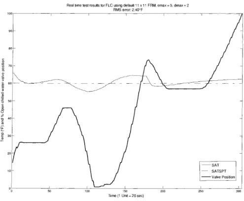
6.1.2 Real-time test results for 121 rules FRM 90
6.1.3 Summary 94
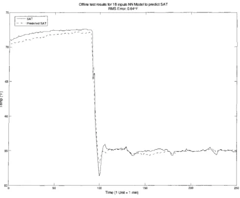
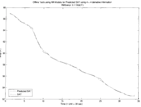
6.2 Neural Network Model Results for predicting SAT 94
6.2.1 Offline Neural Network Models 94
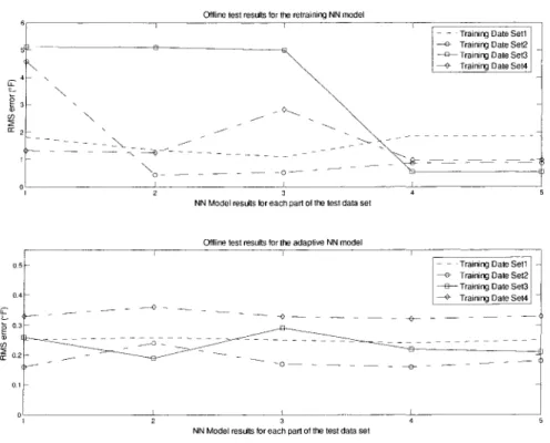
6.2.2 Real-time Test Results for NN Models and Adaptive NN Model 104
6.2.3 Summary 110
6.3 GRNN Model Results for predicting SAT 110
6.3.1 Offline Test Ill
6.3.2 Real-time Test 113
6.3.3 Summary 115
6.4 Lump Capacitance Models Results for predicting SAT 115
6.4.1 Offline Test 116
6.4.3 Summary 119 6.5 Real-time Test Result Comparison for Predicting SAT using Different Models. 119
6.6 Summary 124
Chapter 7 Results for Adaptive Fuzzy Logic Controller (AFLC) 125
7.1 AFLC using Genetic Algorithms (AFLC-GA) 125
7.1.1 FRM obtained by Random Numbers Generated between 1 through 11 126 7.1.2 Changing Human FRM by Random Numbers Generated without changing
Specific Elements 129
7.1.3 Changing Human FRM by Random Number Generated without changing
Specific Elements in the Outer Loop 133
7.2 Summary 136
7.3 AFLC using Evolutionary Strategies (AFLC-ES) 137
7.3.1 Offline Test Results for AFLC-ES with evolving Scaling Factor 139 7.3.2 Real-time Test Results for AFLC-ES with evolving Scaling Factor 140 7.3.3 Offline Test Results for AFLC-ES with evolving Mapping Factor 141 7.3.4 Real-time Test Results for AFLC-ES with evolving Mapping Factor 142
7.4 Summary 143
Chapter 8 Comparison test results for AFLC-GA/ES and PIDL 145
8.1 Introduction 145
8.2 Comparison Test Results for Variation in SATSPT with AFLC-GA on AHUA. 148
8.2.1 RMS Error 150
8.2.2 Hydronic Energy 153
8.2.3 Actuator Travel Distance 155
8.2.4 Rise Time, Overshoot and Setting Time 156
8.3 Comparison Tests Results for Variations in SACFM with AFLC-ES on AHUA 161
8.3.1 RMS Error 166
8.3.2 Hydronic Energy 168
8.3.3 Actuator Travel Distance 169
8.3.4 Rise Time, Overshoot and Settling Time 173
8.4 Comparison test results for variation in SACFM using AFLC-ES on AHUB 175
8.4.1 RMS Error 176
8.4.2 Hydronic Energy 178
8.4.3 Actuator Travel Distance 179
8.4.4 Rise Time, Overshoot and Settling Time 184
8.5 Summary 185
Chapter 9 Conclusions 187
9.1 Details 187
9.2 Contributions 189
9.3 Recommendations 190
Appendix A ERS-Air Handling Unit and Cooling Coil Specifications 191
Appendix B DDE 195
Appendix C Fuzzy Logic 197
Appendix D Neural Networks 207
Appendix F Genetic Algorithms 218
Appendix G Evolutionary Strategies 223
Appendix H ERS System Test Setup 225
List of Tables
Table 1.1-1: Technologies in each category selected for further study 1 Table 1.1-2: Technologies in each category selected for further study continued 2
Table 2.2-1: Stages of lighting load 17
Table 2.2-2: Stages of baseboard heater thermal load 17
Table 2.6-1: Performance Indices for Hydronic Energy in Cooling Tests 23 Table 2.6-2: Performance Indices for Actuator Travel Distance in Cooling Tests 23
Table 2.7-1: Commanded and real chilled water valve position 25
Table 2.7-2: Flow ratio for different chilled water valve position 28
Table 4.3-1: GRNN Models 46
Table 5.1-1: Default 7x7 Fuzzy Rule Matrix 60
Table 5.2-1: Default 9x9 Fuzzy Rule Matrix 62
Table 5.2-2: Default 11x11 Fuzzy Rule Matrix 63
Table 5.2-3: Modified Fuzzy Logic Rule Matrix (11 by 11) 64
Table 5.3-1 : Problem Representation of scaling factor problem for ES 77
Table 5.3-2: 7x7 Human FRM 80
Table 5.3-3: Modified 7x7 Human FRM 81
Table 6.2-1: Offline test results for retraining and adaptive trained neural network model. 100 Table 6.3-1: Results for Offline Tests using GRNN Models for Predicted SAT Ill Table 6.3-2: Offline tests results for predicting SAT using GRNN Models 112 Table 6.3-3: RMS error for predicting SAT using GRNN models II and III 115 Table 6.4-1: RMS error for offline test in predicting SAT using different LCMs 117
Table 6.4-2: RMS error for real time study using LCM IV 119
Table 6.5-1: RMS error for real-time test in predicting SAT using different models 121 Table 7.1-1: Numeric representations of control action (u) for each FMF 125 Table 7.1-2: Best FRM generated by random numbers for offline test 126 Table 7.1-3: Best FRM generated by random numbers for real-time test 128 Table 7.1-4: FRM generated by changing Human FRM by random numbers 130 Table 7.1-5: FRM generated by changing Human FRM without changing specific elements
from the Human FRM 132
Table 7.1-6: FRM generated by modifying elements in the Human FRM without changing
elements in the outer loop 134
Table 7.1-7: FRM generated without changing elements in the outer loop of the Human FRM
for real-time study 135
Table 7.3-1: Maximum and Minimum values for each mapping factor 138 Table 7.3-2: RMS error for real-time test with ES evolving scaling factor 140 Table 7.3-3: RMS error resulted for real-time study of scaling factor 143 Table 8.2-1: Comparison of RMS error/cycle between S for variation in SATSPT test 151 Table 8.2-2: Comparison of hydronic energy/cycle for variation in SATSPT test 153 Table 8.2-3: Comparison of actuator travel distance/cycle for variation in SATSPT test... 155 Table 8.2-4: Case I - Comparison ofcontrol parameters for variation in SATSPT test 158 Table 8.2-5: Case II - Comparison of control parameters for variation in SATSPT test 159 Table 8.2-6: Case III - Comparison of control parameters for variation in SATSPT test... 160 Table 8.3-1: Comparison of average hourly RMS error for variation in SACFM test 166 Table 8.3-2: Comparison of average hydronic energy/hr for variation in SACFM test 168
Table 8.3-3: Comparison of total actuator travel distance/hr for variation in SACFM test. 170 Table 8.3-4: Comparison of performance indices for variation in SACFM test 172 Table 8.3-5: Percentage difference in performance indices for variation in SACFM test... 172 Table 8.4-1: Comparison of average hourly RMS error for variation in SACFM test 176 Table 8.4-2: Comparison of average hydronic energy/hr for variation in SACFM test 178 Table 8.4-3: Comparison of total actuator travel distance/hr for variation in SACFM test. 180 Table 8.4-4: Comparison of performance indices for variation in SACFM test 182 Table 8.4-5: Percentage difference in performance indices for variation in SACFM test... 182 Table 8.4-6: Percentage difference in hydronic energy/day consumption 183
Table A-l: AHU Specification 191
Table A-2: Cooling Coil Specifications 191
Table A-3: ERS data points and accuracy for the sensors used 192
Table C-l: Truth tables for AND, OR, and NOT operators 198
Table C-2: Sample Data from the ERS AHUA 204
Table E-l: Base Case and Variation in each input for Sensitivity Analysis study 215
List of Figures
Figure 1.4-1: Proposed Adaptive Fuzzy Logic Controller - GA 10
Figure 1.5-1: Proposed Adaptive Fuzzy Logic Controller - ES 11
Figure 2.1-1: Schematic of Energy Resource Station, Ankeny, Iowa 16
Figure 2.3-1: Schematic of Air Handling Unit 18
Figure 2.4-1: Schematic of Cooling Coils 20
Figure 2.5-1 : Data Acquisition System 21
Figure 2.7-1 : Commanded and real chilled water valve position 24
Figure 2.7-2: Commanded Vs actual chilled water valve position 25
Figure 2.7-3: Details for chilled water flow through cooling coil and bypass 26 Figure 2.7-4: Flow ratio of chilled water through the cooling coils to bypass 28 Figure 2.7-5: Variation in the ratio for chilled water flow through cooling coil to bypass.... 29 Figure 3.1-1: Definition of Rise Time, Settling Time and Overshoot 32
Figure 3.1-2: Details for AHU Cooling Coil Instrumentation 33
Figure 4.2-1: Neural Networks 38
Figure 4.3-1: GRNN Model Architecture 45
Figure 4.5-1: Schematic of Cooling Coil (CC) 49
Figure 4.5-2: Steps in development of LCM 53
Figure 4.5-3: Flow chart to find optimal values of constants used in LCM 55
Figure 5.1-1: Fuzzy Membership Function (FMF) for Error 59
Figure 5.1-2: Fuzzy Membership Function for Derivative of Error 59
Figure 5.1-3: Fuzzy Membership Function for Control Signal 59
Figure 5.2-1: Modifying shapes of the fuzzy membership functions 65
Figure 5.2-2: Effect of modifying Scaling Factor 66
Figure 5.3-1 : Flow chart for Evolutionary Strategies 69
Figure 5.3-2: Flow chart for evolving scaling factor using ES 70
Figure 5.3-3: Representation of scaling factor problem for ES 71
Figure 5.3-4: Mapping of uniform FMF to non-uniform FMF 73
Figure 5.3-5: Defining FMF in three variables 73
Figure 5.3-6: Uniform fuzzy membership functions in error and derivative of error 74
Figure 5.3-7: Flow chart for evolving mapping factor using ES 76
Figure 5.3-8: Mapping of Uniform FMFs to Non-uniform FMFs in error 79
Figure 5.3-9: Flow chart for GA 82
Figure 5.3-10: Illustration for GA search results 84
Figure 6.1-1: Real-time test results for FLC using default 49 rules FRM 87 Figure 6.1-2: Real-time test results for FLC using default 49 rule FRM 88 Figure 6.1-3: Case I - Real-time test results for FLC using modified 49 rules FRM 89 Figure 6.1-4: Case II - Real-time test results for FLC using modified 49 rules FRM 90 Figure 6.1-5: Real-time test results for FLC using default 11x11 rules FRM 91
Figure 6.1-6: Case I - Real-time test results for FLC 92
Figure 6.1-7: Case II - Real-time test results for FLC 92
Figure 6.1-8: Real-time test results for FLC using modified 11 by 11 elements FRM 93 Figure 6.2-1: Offline test results using NN model with 18 inputs 96 Figure 6.2-2: Offline test results using NN model having derivative information 97
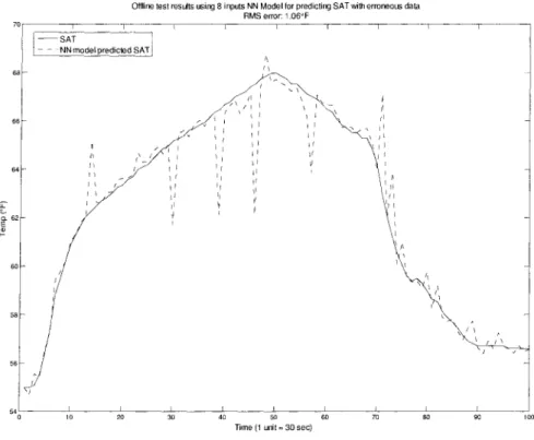
Figure 6.2-3: Offline test result using NN model with 8 inputs for unseen data 98 Figure 6.2-4: Offline test results using retraining & adaptive NN model 101
Figure 6.2-5: Offline test results using retraining NN model 102
Figure 6.2-6: Offline test results using adaptive NN model 102
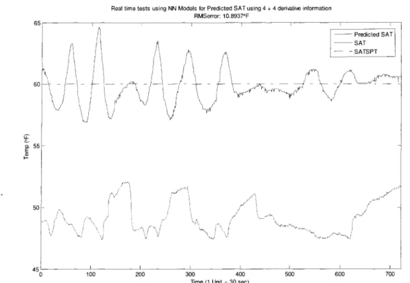
Figure 6.2-7: Offline test result using NN model with 8 inputs having erroneous data 103 Figure 6.2-8: Offline test result using NN model with 8 inputs without erroneous data 104 Figure 6.2-9: Real-time test results using NN model with 18 inputs 105 Figure 6.2-10: Real-time test results using NN model with derivative information 106 Figure 6.2-11: Case I - Real-time test results using NN model using 8 inputs 107 Figure 6.2-12: Case II - Real-time test results using NN model using 8 inputs 107 Figure 6.2-13: Real-time test results for predicting SAT using adaptive NN model 108 Figure 6.2-14: Real-time test results for predicting SAT using adaptive NN model 109 Figure 6.3-1: Offline test results for predicting SAT using GRNN models I and II 112 Figure 6.3-2: Offline test results for predicting SAT using GRNN model I, II and III 113 Figure 6.3-3: Variation in the inputs for real-time testing of GRNN model II and III 114 Figure 6.3-4: Real-time test results for predicting SAT using GRNN models II and III 114 Figure 6.4-1 : Difference between SATPRED and SAT for different LCMs 116 Figure 6.4-2: Variation in the inputs for real-time test using LCM IV 118 Figure 6.4-3: LCM IV predicted SAT and actual SAT for real time test 118 Figure 6.5-1: Variation in the inputs for SAT predicting models study 120 Figure 6.5-2: Real-time test results for predicted SAT using GRNN I and GRNN II 120 Figure 6.5-3: Errors for real-time tests in predicting SAT using different models 121 Figure 6.5-4: Real-time results for predicting SAT using LCM IV and GRNN model II ... 122 Figure 6.5-5: Real-time results for predicting SAT using LCM IV and GRNN model II.... 123 Figure 6.5-6: Real-time results for predicting SAT using LCM IV and GRNN model II.... 123 Figure 7.1-1: Offline test results for the best generated FRM by random numbers 127 Figure 7.1-2: Real-time test results using FRM generated by random numbers 129 Figure 7.1-3: Offline test results for FRM generated by changing Human FRM by random numbers generated amongst -1,0, and 1 without changing specific elements 131 Figure 7.1-4: Real-time test results using FRM generated by changing Human FRM using random numbers generated amongst -1,0, and 1 without changing specific elements 133 Figure 7.1-5: Offline test results using FRM generated by modifying elements in the Human
FRM without changing elements in the outer loop 134
Figure 7.1-6: Real time test results for AFLC-GA with FRM generated by modifying the Human FRM without changing elements in the outer loop of the Human FRM 136
Figure 7.3-1: Offline test results using scaling factor 140
Figure 7.3-2: Real time test results with varying scaling factor 141 Figure 7.3-3: Offline test results for AFLC with evolving mapping factor 142 Figure 7.3-4: Real-time test results for AFLC-ES with evolving mapping factor 143
Figure 8.1-1: Lighting load schedule in the zones 147
Figure 8.1-2: Baseboard load schedule in the zones 147
Figure 8.1-3: Total load schedule in the zones 148
Figure 8.2-1: Comparison test results for variation in SATSPT 149
Figure 8.2-2: Zoom-in comparison test results for variation in SATSPT 149 Figure 8.2-3: Zoom-in comparison test results for variation in SATSPT 150
Figure 8.2-4: Comparison of RMS error/cycle for variation in SATSPT test 152 Figure 8.2-5: Comparison of RMS error/cycle with trend line for variation in SATSPT.... 152 Figure 8.2-6: Comparison of average hydronic energy/cycle for variation in SATSPT test 154 Figure 8.2-7: Comparison of actuator travel distance/cycle for variation in SATSPT test ..156 Figure 8.2-8: Variation in SAT for AHUA (AFLC-GA) and AHUB (PIDL) 157 Figure 8.2-9: Case I - Comparison of control parameters for variation in SATSPT test 158 Figure 8.2-10: Case II - Comparison of control parameters for variation in SATSPT test.. 159 Figure 8.2-11: Case III - Comparison of control parameters for variation in SATSPT test. 160
Figure 8.3-1: SACFM schedule 161
Figure 8.3-2: Comparison test results for variation in SACFM 162
Figure 8.3-3: Zoom-in comparison test results for variation in SACFM 162 Figure 8.3-4: Zoom-in comparison test results for variation in SACFM 163 Figure 8.3-5: Variation in S ATA (AFLC-ES) and SATB (PIDL) and SACFM schedule... 163 Figure 8.3-6: SATA and SATB along with variation in the SACFM for 3rd test day 164 Figure 8.3-7: SATA and SATB along with variation in the SACFM for 4th test day 164 Figure 8.3-8: SATA and SATB along with variation in the SACFM for 5th test day 165 Figure 8.3-9: SATA and SATB along with variation in the SACFM for 6th test day 165 Figure 8.3-10: Comparison of average hourly RMS error for variation in SACFM test 167 Figure 8.3-11: Comparison of average hydronic energy/hr for variation in SACFM test.... 169 Figure 8.3-12: Comparison of actuator travel distance/hr for variation in SACFM test 171 Figure 8.3-13: Percentage difference in performance indices for variation in SACFM test 173 Figure 8.3-14: Case I - Comparison of control parameters for variation in SACFM test.... 174 Figure 8.3-15: Case II - Comparison of control parameters for variation in SACFM test... 174 Figure 8.3-16: Case II - Comparison of control parameters for variation in SACFM test.. 175 Figure 8.4-1: Comparison of average hourly RMS error for variation in SACFM test 177 Figure 8.4-2: Comparison of average hydronic energy/hr for variation in SACFM test 179 Figure 8.4-3: Comparison of total actuator travel distance/hr for variation in SACFM test 181 Figure 8.4-4: Percentage difference in performance indices for variation in SACFM test.. 183 Figure 8.4-5: Comparison of control parameters for variation in SACFM test 184
Figure C-l: Triangular Membership Functions 199
Figure C-2: Basic configuration of Fuzzy Logic System 200
Figure C-3: Centroid Defuzzification Method 202
Figure C-4: Membership Functions for Error 203
Figure C-5: Membership Functions for derivative of error 203
Figure C-6: Membership Functions for Control Signal 203
Figure C-7: Defuzzification of Output (Centroid Method) 205
Figure D-l: Simple Neuron Network 207
Figure D-2: Hard-Limit Transfer Function 208
Figure D-3: Liner Transfer Function 208
Figure D-4: Tan-Sigmoid Transfer Function 209
Figure D-5: Neuron with Multiple Inputs 209
Figure D-6: Generalized Neural Network with a single Hidden Layer Architecture 209
Figure D-7: General Function Approximator 211
Figure E-2: Training Data Distribution - II 214
Figure E-3: Results for Sensitivity Analysis Study 216
Nomenclature C heat capacity rate, (Btu/lbm-°F);
cp specific heat, (Btu/lbm -°F) Cr heat capacity ratio
d derivative of error (°F/sampling period) D; distance function of the input space e error (°F)
f(x, y) continuous probability density function h enthalphy, Btu/lbm
i sample data point
ke, ki starting time, ending time Mp Overshoot (seconds) n initial guesses
n umber of data patters/points nda number of moles of dry air nw number of moles of water vapor p total mixture pressure
Pda partial pressure of dry air pm partial pressure of water vapor
pros pressure of water vapor in saturated moist air Piosin water vapor saturation pressure, psia;
q heat transfer rate, Btu/hr Q volumetric flow rate, ftVmin
QbypaSS Chilled water flow through bypass section (gpm) Qcoi| Chilled water flow through the cooling coil (gpm) Qflow chilled water flow from pump (gpm)
R universal gas constant, 1545.32 ft*lb(/lb mol*°R RMS error0 RMS error for offspring gene
SFemax maximum value of scaling factor SFemin minimum value of scaling factor SFeu pdate Updating value of scaling factor
T Temperature (°F)
T Matrix Transpose
Tabs Temperature (°R) tr rise time (seconds) ts settling time (seconds)
u control action (% change in the chilled water valve position) UA overall heat transfer coefficient, Btu'hr-°F
v specific volume of air leaving from chilled water cooling coil, ft3/lbm
V volume, ft3
VLV actuator position, % Open
X, Y measured values
x,y measured variables
Pi design variables
8 effectiveness
a sample probability of width
cp relative humidity
to humidity ratio lbw a t er/lbdryair
Q ohms A vector A power subscripts a air da dryair min minimum max maximum ma mixed air ra return air
sa ss w supply air steady state water
Experimental Nomenclature
AHUA Air Handling Unit
CC cooling coil
CHWC-DAT cooling water coil discharge air temperature (°F)
CHWC-EWT/EWT entering chilled water temperature into the cooling coils CHWC-LWT/LWT leaving chilled water temperature from the cooling coils CHWC-MWT/MWT mixed chilled water temperature (°F)
CHWC-VLV/VLV chilled water coil value position (% Open) CHWP-GPM/GPM chilled water pump water flow rate (gpm)
exhaust air damper (% Open)
air temperature entering cooling coil (°F)
heating water coil discharge air temperature (°F) air temperature leaving cooling coil (°F)
mixed air temperature (°F) outside air flow rate (cfm) outside air damper (% Open) outside air temperature (°F) return air flow rate (CFM) return air damper (% Closed) return air temperature (°F) supply air flow rate (cfm)
supply air flow rate set point (cfm) supply air temperature (°F)
supply air temperature for AHUA (°F) supply air temperature for AHUA (°F) Supply air temperature set point (°F) EA-DMPR EAT/ OA-TEMP HWC-DAT LAT MAT OA-CFM OA-DMPR OAT/OA-TEMP RA-CFM RA-DMPR RAT/ RA-TEMP SACFM/CFM SACFM-SPT SAT SATA SATB SATSPT
List of Acronyms
EMCS Energy Management and Control System ERS Energy Resource Station
ES Evolutionary Strategies EL Fuzzy Logic
FLC Fuzzy Logic Controller
FLC Fuzzy Logic Controller/Control FMF Fuzzy Membership Functions FRM Fuzzy Rule Matrix
GA Genetic Algorithms
GRNN General Regression Neural Networks LCM Lump Capacitance Model
NL Negative Large fuzzy membership function NM Negative Medium fuzzy membership function NN Neural Networks
NS Negative Small fuzzy membership function NVS Negative Very Small fuzzy membership function
PIDL Proportional Derivative and Integral Loop Controller/Control PIDL Proportional Integral Derivative loop
PL Positive Large fuzzy membership function. PL Proportional and Integral Controller/Control PM Positive Medium fuzzy membership function PS Positive Small fuzzy membership function PVS Positive Very Small fuzzy membership function RMS Root mean square
RTD Resistance Temperature Detectors SF Scaling Factor
TES Thermal Energy Storage
VAV Variable air volume
Acknowledgement
I gratefully thank my advisor Professor Ron M. Nelson for his helpful advice, ceaseless patience, endless support, and heartening encouragement throughout the course of this study. Without his inspiration, this study would not be completed.
I would like to give acknowledgement for the valuable assistance from the people at the Iowa Energy Center and Energy Resource Station including Curt Klaassen, David Perry, and Xiao Hui Zhou. The financial support of the Iowa Energy Center for this research project is sincerely acknowledged. I would also like to thank the members of my thesis committee for their contribution to this work.
I appreciate my teachers, my colleagues and my friends for their helpful discussions, suggestions and encouragement.
Finally, I give my most special thank and express my deepest gratitude towards my parents, my brother, Atul, and my beloved wife, Swarada, for their constant love, patience, care, support, understanding and presence throughout this study and support in my life.
Abstract
An adaptive approach to control a cooling coil chilled water valve operation, called adaptive fuzzy logic control (AFLC), is developed and validated in this study. The AFLC calculates the error between the supply air temperature and supply air temperature set point for air in an air handling unit (AHU) of a heating, ventilating, and air conditioning (HVAC) system and determines optimal fuzzy logic parameters to minimize the error between the supply air temperature and its set point. The AFLC uses genetic algorithms and evolutionary strategies to determine the fuzzy rule matrix and fuzzy membership functions for an AHU in HVAC systems. It is shown that the AFLC can reduce hydronic energy consumption while
maintaining occupant comfort.
Cooling coil models are developed using neural network, general regression neural network and lump capacitance methods to predict the supply air temperature. These models helped with the development of the adaptive fuzzy logic controller.
Two types of validation experiments were conducted, one with cyclically changing supply air temperatures and the second with cyclically changing supply air flow rates. Experiments conducted on two identical real HVAC systems were used to compare the performances of the AFLC to a conventional proportional, integral and derivative (PID) controller. To remove bias between the testing systems, the controllers were switched from one system to the other.
The validation experiments indicate that the HVAC system operated under the AFLC
consumes 1 to 7 % less hydronic energy when compared with a conventional PID controlled system. More actuator travel distance was observed when using the AFLC. The AFLC maintained better occupant comfort conditions when compared with the conventional PID controller. It was observed that the controlled variable for the AFLC system required 0 to 185% more rise time, had 9 to 68% less overshoot and required 11 to 45% less settling time as compared to the conventional PID controlled system.
Chapter 1 Introduction
1.1 Background/Literature Review
The increasing demand for energy efficient buildings has created a need for more energy efficient heating, ventilation, and air-conditioning (HVAC) equipment and systems along with the need to operate and control these systems in the most energy efficient manner. Space heating and cooling is the largest energy expense in most homes, accounting for more than 44% of the average home's utility bill (EERE, 2005). About 32% of the electricity generated in the United States is consumed to heat, cool, ventilate and light commercial buildings (ASHRAE 2000).
U.S. Department of Energy, Office of Energy Efficiency and Renewable Energy published a report on energy savings potential for building technologies program in July 2002. Out of 55 different technologies studied, 15 technologies, shown in Table 1.1-1, were selected for further study based on energy saving potential and the value of further study toward improving estimates of ultimate market-achievable energy savings potential, notably energy savings potential, current and potential future economics, and key barriers facing each option.
Table 1.1-1: Technologies in each category selected for further study (EERE, 2002)
Category Technology for further study
Component Electronically Commutated Permanent Magnet Motor (ECPM) Improved Duct Sealing
MicroChannel Heat Exchanger Smaller Centrifugal Compressors Equipment
Enthalpy/Energy Recovery Heat Exchangers for Ventilation Heat Pump for Cold Climates
Table 1.1-2: Technologies in each category selected for further study continued Systems
Dedicated Outdoor Air Systems Displacement Ventilation
Microenvironment (Task-ambient Conditioning) Novel Cool Storage
Radiant Ceiling Cooling/Chilled Beam Variable Refrigerant Volume/Flow
Controls / Operations
Adaptive/Fuzzy Logic HVAC Control
System/Component Performance Diagnostics
Adaptive/Fuzzy Logic Controls was one of these 15 technologies and had a technical energy savings potential of 0.23 quads which is about 5% of HVAC energy use (EERE, 2002).
Several studies have been reported about the application of adaptive fuzzy logic control. This literature review focuses on the development and validation of adaptive fuzzy logic controllers, self-tuning methods, artificial neural networks, and genetic algorithms. Studies that relate to building energy applications are emphasized.
1.1.1 Fuzzy Logic Controllers
Fuzzy Logic Controllers (FLCs) are based on a set of fuzzy control rules which make use of people's common sense and experience. The fuzzy logic used in these controllers is very well defined mathematically and is able to take into account the uncertainty in the knowledge used to develop the rules and the uncertainty in the operating conditions. The initial rules for FLCs come from the experience of people who work with the systems that are to be controlled. This experience is obtained in the form of linguistic rules such as "If the temperature is too low, open the hot water valve" and "If the temperature is too low and going down fast, open the hot water valve very quickly", etc. These initial rules are then used to construct a fuzzy control matrix that implements the logic of the controller.
The initial fuzzy control matrix and other FLC parameters need to be refined using adjustment strategies that are usually based on manual trial and error methods to achieve improved performance (Huang and Nelson 1991, 1993, 1994a, 1994b). Several researchers have studied and implemented self-tuning or adaptive fuzzy logic controllers (AFLCs) that improve their performance as they adjust to the controlled process and the environment. The operation of an AFLC relies on past experience that looks at suitable combinations of control strategies (control rules, membership functions, and scale factors) and the effects they produce. A particular feature of AFLCs is that they automatically improve their performance until they converge to a predetermined optimal condition.
The first AFLC suggested evaluating and modifying the control rules by a self-organizing algorithm (Mamdani 1979). Several other types of AFLCs have been proposed by researchers (Xu 1987, Shao 1988, Tansheit 1988, Acosta 1992, and Lee 1992). Most of these AFLCs use the tracking error and derivative of error at every sampling instant as the basis not only for the control algorithm but also for the adaptive algorithm. The control action is improved as it is created. The control outputs often become bang-bang signals and convergence of the modifying process is usually slow.
A self-tuning controller for HVAC systems was presented by Wallenborg (1991). A new algorithm for a self-tuning controller was developed in which a discrete time process transfer function was calculated from the wave form of a periodic oscillation obtained with a relay feedback tuning experiment. A general linear discrete time controller was designed using pole placement based on an input-output model. A substantial reduction in commissioning time was achieved compared with manual tuning of conventional controllers.
A computer simulation was studied by Huang and Nelson (1991) to test a new PID control algorithm developed using a fuzzy rule based system. The results showed impressive performance of the PID law combining fuzzy controller for HVAC applications.
Self tuning control with fuzzy rule based supervision for HVAC applications was studied by Ling et al. (1991). The performance of combinations of fuzzy rule based supervisor and self tuning controller was evaluated using a detailed component based simulator developed to test building energy management systems.
Rule development and adjustment strategies of a fuzzy logic controller (FLC) for an HVAC system were analyzed and experimentally evaluated by Huang and Nelson (1993, 1994a, 1994b) for controlling a pneumatic valve to control the temperature of hot water to a hot water coil.
Some modern control strategies were applied to a HVAC system. Zaheer-uddin (1993) used a multivariate control design in a water heating system. The optimal regulator design was applied for damper control of the supply air to a single zone. The sub-optimal operation was employed in a single zone with a heating coil for a constant air volume (CAV) system. The model reference adaptive control was applied to a single zone with a cooling coil for a variable air volume (VAV) system (Zaheer-uddin 1993). Simulation results showed that these modern control strategies were stable.
The neural network method was applied to a HVAC system for the first time by Curtiss et al. (1993, 1994 and 1996). A hot water coil that was used to heat air was modeled by two types of ANN s and a predictive controller was combined with the ANN to develop a future adaptive neural network (FANN) control. Simulation and experimental results show that the F ANN control has a better behavior when compared with PID control. Work of Curtiss was expanded by Jeannette et al. (1998) to test the predictive Neural Network (PNN) in a real building. More experiments were conducted to obtain good control of the hot water supply temperature using a predictive NN. Results for energy savings were not reported.
A self-tuning control algorithm was developed by Ozsoy (1993). The algorithm combined the recursive parameter estimation method with control algorithms. The algorithm was applied to a single environmental space with an air heater, humidifier and ventilator system.
Simulation results showed that the algorithm had a robust behavior. Results for energy savings were not reported.
Arima (1995) applied fuzzy logic and rough sets for heating and humidification controls. Experimental results showing better performance of fuzzy logic reasoning are presented. No information on how the fuzzy rule matrix was developed or how they were tuned is presented.
Ying-guo Piao et al. (1995) and Arima et al. (1995) developed an FLC for controlling the temperature of hot water provided to a heating coil. Results for energy savings were not presented.
So et al. (1995) introduced a controller using a system identification method. The controller was able to predict the new system status based on the past records and suggested optimal control actions. Simulation results showed that the proposed controller behaved better than a conventional PID controller when both controllers were used to control an AHU system. Energy savings of about 6.62% were demonstrated by using the proposed controller.
A new pattern recognition adaptive controller that had the ability to self-tune PID parameters was described by Seem (1998). The controller was computationally efficient and provided near optimal performance. The controller was successfully used in many real buildings and showed good control of the HVAC system. Results for energy savings were not reported.
An adaptive learning algorithm based on genetic algorithms (GAs) for automatic tuning of PID controllers in HVAC systems to achieve optimal performance was presented by Huang (1997). The simulation results showed that genetic algorithm based optimization procedures are useful for automatic tuning of PID controllers for HVAC systems, yielding minimum overshoot and minimum settling time.
Velez-Reyes and Arguello-Serrano (1999) presented a nonlinear controller with a thermal load estimator for the HVAC system. The controller was capable of identifying time varying thermal loads. This capability enabled the controller to have better control when the system endured a large thermal load disturbance. The controller was used in a HVAC system. Better control of the nonlinear controller was demonstrated by simulation results. Results for energy savings were not reported.
Jian (2000) developed an Adaptive Neuro-Fuzzy (ANF) method for the supply air pressure control loop of a HVAC system. The ANF controller was developed to overcome the weakness of a well-tuned PID controller, which performs well around normal working points, but its tolerance to process parameter variations was severely affected due to the limitations of PID controllers for systems that have larger dead times or large parameter variations. No information on the neural network was made available. It was not clear if the controller used neural networks with multiple outputs for updating each membership function parameter in the fuzzy logic part. Also, the membership functions used in the fuzzy logic part were not specified. Also, it was not clear if the neural network was updating membership functions in every step or after a fixed number of steps. Simulation performances were compared without any experimental results.
Osman (2000a and 2000b) developed a feedforward controller using a General Regression Neural Network (GRNN) for controlling the temperature in a laboratory room. This HVAC system used a VAV system. No details about the GRNN model and the data used for training were presented. Simulation results show that by adjusting damper position and supply flow rate, the required room temperature can be achieved.
Wang Qing-Guo (2000) developed an auto-tuning multivariate controller for HVAC systems. In this paper, an advance PID auto-tuner for both single and multi-variable processes was developed with its application for controlling the zone temperature. No cost saving or energy consumption information was presented. No comparison of the PID
auto-tuner to a conventional PID controller was made. Experiments were conducted in a HVAC pilot plant.
Kolokotsa (2001) has developed an advance fuzzy proportional derivative (PD) controller for adjustment and preservation of air quality, thermal and visual comfort for buildings' occupants and achieved a reduction in energy consumption. The adaptive fuzzy PD controller adapts the input and output scaling factors and was based on a second order reference model. The buildings' response to the control signals was simulated using MATLAB/SIMULINK without any experimental results.
Alcala (2003) presented a smartly tuned FLC for an HVAC application which was developed using genetic algorithms. The genetic algorithm was used to obtain better fuzzy rule sets. The problem considered was very particular and complex. Simulation and experimental results showed energy savings. No information related to the test conditions were presented and the tuning method used is very complex.
More work is needed to develop AFLCs for HVAC applications that typically have long (about a minute or so) system time constants and periodically change operating modes (i.e. heating to cooling, using setback, etc.). Having a good adaptive or self-tuning algorithm for fuzzy logic controllers would increase their use, since considerable time is needed to manually tune FLCs. Properly tuned PLCs can be superior to conventional control algorithms (such as Proportional, Integral and Derivative (PID)), because they respond more quickly to setpoint and environmental changes and have minimal overshoot of the controlled variables. The controlled systems reach steady state faster with reduced oscillations about the set point. The quick response improves comfort and, since the systems spend less time in transient operation, energy consumption is reduced. The control logic can also implement electric demand and energy saving measures.
1.1.2 Summary
The literature review in the areas of adaptive fuzzy logic and self tuning controller reveals adaptive techniques that have been applied to both HVAC unit control and system control along with the other industrial problems (Wallenberg 1991, Ling and Dexter, 1991, So et al., 1995). Results for an adaptive controller show stable behavior and better performance compared with conventional control algorithms.
Combining adaptive techniques with optimization techniques leads to minimum overshoot and minimum settling time, thus saving energy (Huang and Nelson, 1999). In recent years, adaptive techniques have been used successfully in simulation studies for HVAC operation.
Several studies (So et al. 1995, Ling and Dexter, 1991, Wang and Jin, 2000) using adaptive control in the HVAC area have demonstrated that adaptive control leads to reduction in energy costs in comparison to conventional control strategies while still maintaining comfort conditions for building occupants.
The literature indicates a lack of applications of simple adaptive techniques that are
combined with optimal operation for cooling coil in HVAC systems. Furthermore, most of the current studies stop at the simulation level and do not present results for experiments and energy savings data.
1.2 Project Objectives
The objective of this project is to develop, implement, and test an adaptive fuzzy logic controller on one of the air handling units at the Iowa Energy Center's (IEC) Energy Resource Station (ERS) located in Ankeny, Iowa.
1.3 The Adaptive FLC description
Over the past couple of years, fuzzy logic has played an important role in the implementation of controllers for various processes. FLCs are effective for controlling complex and poorly defined processes as they embody the knowledge of human experts to achieve good control strategies. Adaptive fuzzy logic control systems have been designed for various dynamic
processes. In a PLC, however, it is difficult to construct good rule bases and membership functions.
Some studies have been reported that use Genetic Algorithms (GAs) for the optimization of PLC performance by overcoming the above mentioned difficulties. Karr (1991) has used genetic algorithms to select good membership functions for a PLC that controlled a computer simulated cart-pole balancing problem. Genetic algorithms were used to alter the shape of fuzzy sets used in a given rule base in which each fuzzy label was coded as a 7-bit binary number.
Recently, Gurocak et al. (1999), Park et al. (2000) have shown the use of genetic algorithms for tuning fuzzy logic controllers for the inverted pendulum problem. Kindel et al. (1994) used modified genetic algorithms for designing and optimizing fuzzy controllers for the cart pole system. The task was divided into rule base modification and tuning of fuzzy membership function shape. They used non-binary coding and coded the rule base as matrix type chromosomes instead of general gene type chromosomes. Borut et al. (1999) used genetic algorithms to tune 25 consequent parameters keeping the membership functions the same. The efficiency of this approached was verified and validated on a hydraulic control system. Park et al. (1995) used genetic algorithms for fine tuning the fuzzy logic controller. The effectiveness of this method was verified through a series of simulations for a water level control system.
1.4 Proposed Adaptive Fuzzy Logic Controller - G A
Figure 1.4-1 shows a schematic of a proposed adaptive fuzzy logic controller using genetic algorithms (AFLC-GA). In this project, Genetic Algorithms (GAs) are used to modify the fuzzy logic controller's rule matrix. Total RMS error between the supply air temperature (SAT) and supply air temperature set point (SATSPT) is calculated for each Fuzzy Rule Matrix (FRM). This total RMS error value is used to evaluate the performance of all the generated FRMs. FRMs that have better PLC performance are reproduced to find improved FRMs. Thus, with the repeated application of GAs, near-optimal fuzzy logic controllers can
be achieved (See Appendix E for details).All the programming required for PLC and GA was done using Matlab software (Matlab 2001).
Control Action SAT
Air Handling Unit (AHU) at the ERS
Genetic Algorithms (To update Fuzzy Rule Matrix (FRM)) Fuzzy Logic Controller
(To generate a control action for given e and d) Adaptive Part
Updated FRM
Data
Figure 1.4-1: Proposed Adaptive Fuzzy Logic Controller - GA
As shown in Figure 1.4-1, for a set of error (e) and derivative of error (d), a control signal will be generated by the FLC. Depending upon the control signal calculated using the current FRM; the chilled water valve position is altered thus changing the SAT. For the offline study, SAT values were calculated using a general regression neural network (GRNN) model for the cooling coil instead of the real Air Handling Unit block as illustrated in Figure 1.4-1. The GRNN model was also developed using Matlab's NN toolkit. After a specified number of iterations of the control cycle are completed, the total RMS error corresponding to the FRM being used is calculated. Similarly, the total RMS error for each FRM generated for the study is calculated to evaluate the FLC performance.
Based on the total RMS error, all the generated FRMs are then sorted with the FRMs having minimum RMS error being best. After the sorting process, the two top most FRMs having minimum total RMS error are used for the reproduction of two new FRMs called offspring. The total RMS error is calculated for these offspring as mentioned above. Depending upon the total RMS error for these offspring namely, none, one or both the worst FRMs from the selected tournament (tournament is selecting either 4 or 7 FRMs randomly from the total generated FRMs) are replaced by the offspring FRMs. This process of generating new FRMs
(i.e. offspring) is continued for a pre-defined number of cycles, called generations. Thus, the best FRM is generated which results in a better performance of the FLC. The same method used for offline test was applied in real time test at the ERS to find a better FRM.
1.5 Proposed Adaptive Fuzzy Logic Controller - ES
Pham et al. (1994) proposed an evolutionary strategy (ES) design of an adaptive fuzzy logic controller for a process with time delays. An adaptive fuzzy logic controller incorporating a Smith predictor was designed to maintain performance during process changes. Simulation results demonstrated the effectiveness of this approach.
Figure 1.5-1 shows a schematic of a proposed adaptive fuzzy logic controller using Evolutionary Strategies (ES). In this method, ES is used to evolve better fuzzy membership functions. The required program of FLC, GRNN model and ES was done using Matlab software.
SAT Action
^ '
Air Handling Unit (AHU) at the ERS Fuzzy Logic Controller
(To generate a control action for given e and d)
Evolutionary Strategy (To update Fuzzy
Membership Functions) Adaptive Part i i Control Updated Fuzzy Membership Functions Data
Figure 1.5-1: Proposed Adaptive Fuzzy Logic Controller - ES
The ES technique is similar to the GA technique as explained in the previous section except that GAs work with many genes at a time and ESs work with only one gene at a time. The task for this research is to develop and implement an adaptive fuzzy control algorithm at the ERS.
1.6 Plan of Work
The plan for this research has been to develop and implement an adaptive fuzzy control algorithm at the ERS. The ERS is an excellent facility to use for testing and developing PLCs for controlling commercial HVAC systems. The ERS has two side-by-side air handling units with identical thermal loads. Each system is controlled by a computerized energy management and control system (EMCS). The EMC S s can be programmed to implement and compare control strategies, such as the fuzzy logic controllers on one air handling unit and other control strategies, such as a standard PID controller, on the second air handling unit.
Tasks which are followed in this research are: 1. Develop and implement a FLC at the ERS
2. Compare performance of FLC with that of current control strategies 3. Develop procedures for dealing with missing and erroneous data 4. Develop and implement an AFLC at the ERS
Task 1 - Develop and implement a FLC at the ERS
For this task, a working fuzzy logic controller was developed, manually tuned, and used to control one of the air handling units. The control variables were selected and initial FLC development was done off-line. Then, real-time (online) experiments were conducted on one of the air handling units (AHU) to test the operation of the FLC.
Task 2 - Compare performance of FLC to current control strategies
The performance of a FLC was compared to the performance of the PIDL (proportional/integral/derivative loop) controller implemented by the EMCS at the ERS. The FLC developed in Task 1 was used to control one of the two identical air handling units and its operation and energy use were compared to the other one which had the PIDL controller. The use of the FLC was periodically switched from one air handling unit to the other to eliminate any bias in one unit over the other. The performance of both the systems in terms
of reduced energy usage, faster response time, reduced overshoot, and reduced oscillations was recorded and compared.
Task 3 - Develop procedures for dealing with missing and erroneous data
Most EMCS s have to deal with missing and/or erroneous data. This is caused by sensor malfunctions and failures or other problems within the computer control system. Poor sensor readings degrade the performance of any control system. There are two types of erroneous data: (1) complete failures and (2) minor drifting. The complete failures can easily be detected by readings that are out of range. Replacing missing and erroneous data with the previous correct value was studied. Also, in future work, Auto Associative Neural Networks will be studied as one of the tools to deal with minor drifting.
Task 4 - Develop and implement an adaptive FLC at the ERS
For this task, an adaptive FLC (AFLC) was developed to automatically tune itself for optimal performance using GA or ES. Once an adaptive FLC was developed, its performance was compared with the PIDL control strategy used at the ERS with each one controlling side-by-side air handling units. Both the systems are compared based on the following evaluation parameters:
1. Error (SAT deviation from the SATSPT) 2. Energy usage
3. Response time to setpoint and environmental changes
4. Overshoot of the controlled variables, settling and rise time required 5. Chilled water valve travel
1.7 Outline of Contents
Chapter 2 is a description of the experimental facility, including information related to building layout, air handling units, cooling coil and data acquisition system. A brief discussion of a bias study between the two systems is reported along with the uncertainty values for hydronic energy and actuator travel distance. A discussion of a chilled water valve position study is also presented. Chapter 3 discusses various performance indices used in this
study. Chapter 4 gives detailed information for the cooling coil model development using neural networks, general regression neural network and lump capacitance models. An introduction to fuzzy logic controllers and adaptive fuzzy logic controllers is discussed in Chapter 5. Experimental results for the manually tuned FLC and various cooling coil models are given in Chapter 6. Chapters 7 reports the results obtained for offline and real time tests for adaptive fuzzy logic performance using genetic algorithms and evolutionary strategies. Chapter 8 reports the results for real-time comparison tests between the adaptive fuzzy logic controller and a standard proportional, derivative and integral loop controller. Finally, conclusions, contributions, and recommendations of this study are given in Chapter 9
Chapter 2 Experimental Facility Description
2.1 Introduction
The Energy Resource Station (ERS) was used as the test facility to compare the AFLC to a conventional PID controller. The ERS was built to compare different energy efficiency measures and to record energy consumption. The ERS combines laboratory testing capabilities with real building characteristics and is capable of simultaneously testing two full-scale commercial HVAC systems side-by-side with identical thermal loadings. This method of performance testing emphasizes the importance of the entire HVAC system and the interactions between individual building elements.
To perform side-by-side testing, the facility is equipped with three AHUs. AHU-1 serves the common areas of the building. The remaining AHUs serve the A and B Test Systems. AHUA and AHUB are identical. AHUA and AHUB each serve four zones which are identical in construction and thermal loads. A schematic of the ERS along with the location of each AHU and the zones are shown in Figure 2.1-1. Of the four zones for each AHU, three have external exposures and one sees only internal conditions. The A and B zones are mirror images of each other. The zones have the capability for identical internal thermal loads.
The side-by-side zones and HVAC systems allow a conventional control methodology to be operated in one system, for example, the A-Test System, and a proposed control methodology to be operated in the other system, for example, the B-Test System. Because each test system has the identical loads (external and internal) and construction, the only difference in the tests should be the control methodologies. Hence, the energy consumption and other performance indices of the two test systems can be compared and the benefits of the proposed control methodology can be quantified.
AHU-A AHU-B Mechanical Room AHU-1 Classroom Classroom Int Display Room Media Center Served by AHU-1 West A Served by AHU-A Served by AHU-B Offices & Computer Center Reception South South Office
Figure 2.1-1: Schematic of Energy Resource Station, Ankeny, Iowa.
2.2 Thermal Loads
Each zone is equipped with 2-stage baseboard electric heaters and overhead lighting. The baseboard electric heaters and lighting can be scheduled to simulate various usage patterns as shown in Table 2.2-1 and Table 2.2-2. These zones are equipped with 2-stage lighting that can be in one of three modes shown in Table 2.2-1 with the corresponding thermal load generated in each stage. Also zones are equipped with 2-stage baseboard heater that can be in one of three modes shown in Table 2.2-2 with the corresponding thermal load generated in each stage. The lighting and baseboard heater thermal load was used in this study.
Table 2.2-1 : Stages of lighting load Lighting
Mode Stage Power
1 2 (W)
1 ON OFF 195
2 OFF ON 390
3 ON ON 585
Table 2.2-2: Stages of baseboard heater thermal load Baseboard Heater
Mode Stage Power
1 2 (kW)
1 OFF OFF 0
2 ON OFF 1
3 ON ON 2
2.3 Air Handling Unit
A schematic of the AHUs with the major components is shown in Figure 2.3-1. Major components shown are the supply air and return air fans, preheat, cooling, and heating coils, heating and cooling control valves, recirculated air, exhaust air, and outdoor air dampers, and the ducts to transfer the air to and from the conditioned spaces. The preheat coil was not used in this study. The equipment capacities for the components of the AHUs are listed in Appendix A.
Instrumentation consisting of humidity, pressure, and temperature sensors, air flow stations, and electric power meters are available to monitor the operational characteristics of the AHUs. The accuracy of the sensors as stated by the sensor manufacturer are listed in Appendix A.
Exhaust air Outdoor OAT air Return fan RFWAT
XX
RAT EADP <3 oa Return air ra Recirculated air OACFM RADP d SAT OADP Heatedwater Chilled water
HCWLWT CHR'CLM
Figure 2.3-1: Schematic of Air Handling Unit (Wen 2003)
Referring to Figure 2.3-1, outdoor air at temperature OAT enters the AHU through the outdoor air duct and mixes with recirculated air at temperature RAT to form mixed air at temperature MAT. The OAT, MAT and RAT are measured with average temperature arrays of 4 platinum 1000 Q RTD temperature probes connected to form a single average 1000 Q RTD input. The mixed air passes through the heating coil and cooling coil at supply flow rate of SACFM. The air passes through a cooling coil where heat is removed from the air.
The cooling coil was designed for a nominal capacity of 140 kBtu/hr. The discharge air temperatures of the heating and cooling coils (HWCDAT and CHWCDAT) are measured with average temperature arrays of 4 platinum 1000 Q RTD temperature probes connected to form a single average 1000 £2 RTD input. The flow rate of chilled water through the cooling coils is controlled by varying the position of the three-way heating and cooling valves.
The air is drawn through the supply fan. The speed of the supply fan is controlled with a variable frequency drive (VFD). The electrical power for the supply fan and VFD is
measured with an electric power transducer. The air flow rate of the supply air (SACFM) is measured at the supply air flow station and the supply air temperature (SAT) is measured with an RTD average temperature array. The humidity of the supply air (tpsa) is measure using a humidity probe. The supply air is distributed to the zones through the supply air duct.
An Energy Management and Control System (EMCS) is a Johnson Controls Inc. (JCI) Metasys system (JCI, 1995) used to regulate the conditions within the AHU by providing signals to maintain SAT at the supply air temperature set-point (SATSPT).
2.4 Cooling Plant
The cooling plant consists of a nominal 10 ton air-cooled chiller, a 149 ton thermal energy storage (TES) unit, chilled water supplied from an outside source, pumps, necessary valves and piping to circulate chilled water through the HVAC components. The TES unit is not used as an energy storage device, but acts as a large capacitance that reduces the temperature oscillations of the chilled water supplied to the cooling coil.
Instrumentation consisting of flow meters, immersion temperature probes, electric power meters, and pressure sensors are available to monitor the operational characteristics of the cooling plant. Equipment capacity for each of the components of the chilled water system is listed in Appendix A. The working fluid in the cooling plant is water with 15% ethylene glycol.
Figure 2.4-1 shows a schematic of the cooling coils. The chilled water generated by the local chiller is supplied to the cooling coils in AHUA and B. The chilled water generated from the local chiller is allowed to pass through the TES unit, which is filled with water to stabilize the temperature fluctuations generated by the stage controlled local chiller. The various temperature probes are shown in Figure 2.4-1 measure the entering, leaving, and mixed water temperatures to cooling coil. A flow meter measure the flow of the chilled water through the cooling coils.
Entering Chill Water Leaving Chill Water CHWC-MWT Flow Meter Actuator CHWC-EWT CHWC-LWT EAT SAT Cooling Coil
Figure 2.4-1: Schematic of Cooling Coils
CHWC-EWT - Chilled Water Entering Temperature (°F) CHWC-LWT - Chilled Water Leaving Temperature (°F) CWC-MWT - Chilled Water Mixed Temperature (°F) EAT - Entering Air Temperature (°F)
SAT - Supply Air Temperature (°F)
2.5 Data Acquisition
The data exchange between the Matlab program (Matlab 2001) and the EMCS is implemented using a network dynamic data exchange (DDE) (See Appendix B for details) protocol that is supplied by the EMCS manufacturer.
The EMCS is a Johnson Controls Inc. (JCI) Metasys system (JCI 1995). For the communication between Matlab and Metasys, Metalink served as a gateway to get information from Matlab and then deliver it to the Metasys controller. Figure 2.5-1 illustrates Data Acquisition System.
JCI's IV/TÏhT A T TNTf MATLAB
METASYS DDE IVlC 1 A-LllN rv DDE Program
Protocol Protocol
Figure 2.5-1 : Data Acquisition System.
For example when a request for chilled water valve position is made by the Matlab program, this request is communicated to Metasys controller via Metalink using the network DDE protocol. The Metasys controller acquires required information and is communicated to the Matlab program through Metalink using the network DDE protocol. Similarly when a need for change in chilled water valve position is required, the Matlab program communicates this need using a "poke" command on the network DDE protocol to the Metasys controller via Metalink. Once the information for change in the chilled water valve position is received, the Metasys controller executes the required action.
The Matlab program requests values for required sensors, namely various temperatures, chilled water valve positions and damper positions, approximately after every 30 seconds, since little variation in time was observed for completion of each program cycle. One program cycle was defined as starting with the request to the Metasys system for data from the required sensors, obtain that data, calculate the error between SAT and SATSPT and then the derivative of error, calculate the FLC action to change the chilled water valve position, poke this action into the Metasys system to execute, calculate the value of the predicted SAT using different models, namely LCM, NN or GRNN models (to be defined later), and lastly storing all the values in a text file. Time variation in executing every request by Metasys system was observed due network traffic and calculation of control actions using the fuzzy logic program. All the data received from Metasys was stored using Matlab software in a text files.
2.6 Bias Study for System A and System B
Even though test systems A and B were designed to be identical, there are always factors existing in the equipment, installation, and operation that cause the two systems to have different values for the performance indices when the same operation methodology is applied to both the systems. Before conducting the comparison tests, it was necessary to determine the bias between the A and B systems from energy, thermal comfort, and actuator travel distance points of view. It is desired to know:
• The magnitudes of the differences between the performance indices (bias) for the A and B test systems when both systems are under the same operating conditions, and • The repeatability of the bias.
Wen (2003) documented an extensive study for the bias test between the two systems at the ERS. A group of tests, called AOOM normalization tests (AOOMnorm), was developed to serve the purpose of verifying the bias between the A and B test systems. The AOOMnorm tests were configured so that the systems A and B were operated and controlled using the same conditions under PIDL control. Each AOOMnorm test lasted about one week. AOOMnorm was executed ten times to verify the bias for different weather conditions. Results for these tests are given in Table 2.6-1 and Table 2.6-2.
From the results in Table 2.6-1 and Table 2.6-2, it is observed that there is a difference in the hydronic energy consumption and the actuator travel distance for both systems when using the same PIDL control strategy. System B consumed almost 7.5% more hydronic energy than System A and the chilled water valve movement on AHUA was almost 9% more than for AHUB, calculated after excluding the outliers.
The uncertainties due to the measurement errors were also examined by Wen (2003). The uncertainties for the energy performance indices were less than 2% of the minimum performance indices value. The uncertainties for the ATD indices were less than 0.5% of the minimum performance indices value (Wen 2003).
Table 2.6-1: Performance Indices for Hydronic Energy in Cooling Tests (Wen 2003)
Performance Indices for Hydronic Energy in Cooling Test (kBtu) AOOMnorm2.2
Test Day AHUA AHUB
% Difference (B-A)*100/B 1 135.55 147.14 8.6 2 154.01 168.34 9.3 3 120.3 132.92 10.5 AOOMnorm2.10 1 70.79 73.64 4 2 57.25 57.19 0.1 3 84.32 89.58 6.2 4 79.31 84.8 6.9
Table 2.6-2: Performance Indices for Actuator Travel Distance in Cooling Tests
(Wen 2003)
Performance Indices for Actuator Travel Distance in Cooling Test (kBtu)
AOOMnorm2.2
Test Day AHUA AHUB
% Difference (B-A)*100/B 1 311 277 -12 2 374 326 -15 3 421 385 -9 AOOMnorm2.10 1 241 261 -9 2 279 276 -1 3 243 265 -9 4 252 298 -18