On the Probabilities of Correlated Defaults: a First
Passage Time Approach
∗M. Valuˇzis
Department of Mathematics and Informatics, Vilnius University Naugarduko str. 24, LT-03225 Vilnius, Lithuania
Received: 03.09.2007 Revised: 15.01.2008 Published online: 06.03.2008
Abstract. This article investigates the joint probability of correlated defaults in the first
passage time approach of credit risk subject to condition that the underlying firms’ assets values and the default boundaries follow geometric Brownian motion processes. The exact analytical expression of joint probability of two correlated defaults in the case of stochastic default boundaries is presented. Also, some properties of this solution are provided.
Keywords: correlated defaults, joint probability of default, implied correlation.
1
Introduction
Together with the evaluation of loss given default and expected losses of any defaultable financial claim, there is equally important to estimate the cumulative distribution function of correlated defaults. The knowledge of marginal probabilities is not sufficient to assess the credit risk of corporate bonds portfolio due to existing correlation (or interdepen-dence) between the asset returns. Usually, default correlation is defined by correlation between the Brownian motions driving the individual companies and plays a crucial role in determining the joint probability of default, i.e. the probability of multiple defaults. Also, the default correlations are the important factors in order to calculate portfolio risk. In this paper we analyze the credit risk of portfolio of correlated defaultable claims. One of the most important measures of credit risk, the probability of default of one claim is investigated extensively in the literature. However analyzing the credit risk of portfolio, it is also important to measure the joint probability of correlated defaults and the general probability of portfolio default. “Modeling correlated default risk is a new phenomenon
currently sweeping through the credit markets. Due to the rapid growth in the credit derivatives market and the increasing importance of measuring and controlling default risks in corporate bonds portfolios, derivatives, and the other securities, the importance ∗The research was supported by bilateral France-Lithuanian scientific project Gilibert and Lithuanian State Science and Studies foundation (V-07058).
of default correlation (or inter-dependence) analysis has been recognized by the financial industry” (Zhou, [1]). The losses on the initial credit portfolio due to the default of the
underlying firms depend on the default probability of each firm and the losses given default. In addition, the degree of dependence between the firms’ default probability plays an important role on the timing of the firms’ defaults and, as a consequence, on the distribution of the portfolio losses. The correlation between several assets is important for estimating general credit risk of portfolio because higher correlation of defaults implies a greater likelihood that losses will wipe out the assets. Conversely, higher general correlation also makes the extreme case of very few defaults more likely.
In general, the structure of default correlation is a crucial issue in pricing multi-name credit derivatives as well as in credit risk management. In addition, the joint probability of correlated defaults is important for assessment systematic risk of whole financial system due to financial contagion (more about the economic and financial importance of default correlation see, for example [2] and [3]).
Many papers analyzing the default correlation are focused on the joint probability of default in reduced form models, but there are fewer publications concerning the joint probability of correlated defaults in structural approach, notably, [2,4–7] and [1]. Drawing on literature, we noticed that one of the biggest disadvantages of structural models is their limited possibilities of calculating the joint probability of correlated defaults. The aim of this paper is to enlarge this possibility for structural approach of credit risk. We derive the joint probability of two correlated defaults in the case when the default thresholds (in special case the values of bonds) are also stochastic.
In many papers (see, for example, Overbeck and Stahl [8], Zhou [1]) the default correlation is defined as the correlation of Bernoulli distributed random variables. In this paper, we generalize the Zhou’s model for two correlated defaults by defining the more general structure of default correlation. Unlike Zhou [1], Patras [7], Overbeck and Schmidt [6] approaches, in this paper we assume that the value ofi-th default threshold is stochastic without jumps. That means the case when, for example, investors do not have full information about financial markets (notably, some exogenous shocks, depositors panics or other changes) or due to stochastic behavior of interest rates. In fact, by assuming stochastic behavior of default boundary, we also consider other exogenously defined type of financial risk, notably, liquidity and market changes risk. Other economic interpretation is that stochastic default threshold can represent some debt covenant viola-tion. Unlike other structural models with incomplete information, we assume that there are no jumps and that default time of company remains predictable due to the continuity of both stochastic processes and we avoid the further modelling of transformed structural approach to reduced form model with endogenous intensity processes. Also, presented model differs from others by the correlation structure of implied Brownian motions and by the defined structure of this correlation.
The paper is organized as follows. In Section 2 we give a short overview of related literature. In Section 3 we present a generalized first passage time model. In Section 4 we outline the expression of the probability of single default. The closed form expression of the joint probability of correlated defaults is given in Section 5, and in Section 6 we give some conclusions.
2
Overview of the literature
In practice, it is complicated way to find an analytical expression of cumulative distri-bution function of correlated defaults. There are three main approaches to estimate the joint probability of correlated defaults: calculations using credit market historical data (Lucas, [3]), reduced form credit risk approach and structural approach of credit risk which is the less developed in this sense.
Calculation using historical data has some important drawbacks because it is hard to determine whether historical fluctuations in default rates are caused by default correlations or by changes in default probability. Also, there are not enough data concerning the default correlation among and between specific industries and defaultable bonds, it does not use firm-specific information and default correlations are time-varying, so past history may not reflect the current reality. Das and Geng [9] calculated joint probabilities of default for U.S. corporations using credit ratings data for copula functions. They used a metric that compares alternative specifications of the joint default distribution using three criteria: (a) the level of default risk, (b) the asymmetry in default correlations, and (c) the tail-dependence of joint defaults.
In reduced form (or intensity) approach of credit risk this problem has been investi-gated in several ways: models of conditionally independent defaults, models of contagion and copula functions. The intensity models the conditional default arrival rate during some period. These models can incorporate correlations between defaults by allowing hazard rates to be stochastic and correlated with macroeconomic variables. To induce correlation between defaults, one would typically introduce correlation between the in-tensity processes. However the problems begin when one attempts to estimate them. These problems are, in part, due to the lack of sufficiently adequate default information about the dependence structure of the credit risk of the firms under consideration. Their main disadvantage is that the range of default correlations that can be achieved is limited. Even when there is a perfect correlation between two hazard rates, the corresponding correlation between defaults in any chosen period of time is usually very low (for more details, see [3]). The recent so called second generation models that come under the heading of “intensity based top down models” avoid this problem (see, for example, [10]). Moreover, these models, (for more details, see the papers of Davis and Lo [11] and Giesecke and Goldberg [10]) incorporate the contagion observed in credit markets.
Due to their intuitive simplicity, structural approach is more attractive than reduced form approach but one of the biggest problems of application structural models in assess-ment the credit risk of corporate bonds portfolio is the complicated way of estimation of the joint probability of correlated defaults. In structural approach, the default corre-lation between issuers is introduced through asset return correcorre-lation. With predictable defaults, however, jumps in bond prices and credit spreads cannot appear at all: prices converge continuously to their default-contingent values. This means that, although the existing structural models provide important insights into the relation between firms’ fundamentals and correlated default events as well as practically most valuable tools, they fail to be consistent in particular with the observed contagion phenomena. Zhou [1] obtained the closed form expression of the joint probability of correlated defaults in the
case when default boundaries are exponential functions. Zhou derived this formula in both cases: when firm’s asset value and default threshold grow at the same and at the different rates. Overbeck and Schmidt [6] derived similar expression in the case where the underlying ability-to-pay process for each bond is a transformation of Brownian motions with default trend. Patras [7] presented a generalized reflection principle and evaluated digital swap on two credit instruments1in the case when the default boundaries are deterministic functions in planar Brownian motion and the correlation follows Bessel process. Giesecke [2] derived similar formulas in the case of complete and incomplete information. This paper provides a structural model of correlated default which is con-sistent with several significant credit spread characteristics: the implied short-term credit spreads are typically non-zero, credit spreads cyclical correlations across firms, and, most importantly, contagion effects are predicted. Giesecke characterized the joint default probabilities and the default dependence structure as assessed by investors, using the modeling of dependence with copulas for stochastic boundaries. In the paper of He, Keirstead and Rebholz [5] the closed form expressions of the joint probability of the maximum and minimum values of two correlated Brownian motions are derived and applied to the valuation of double lookback and barrier (or knockout) options in the case when hitting boundaries are constants. Fouque, Wignall and Zhou [4] extended the first passage time model by defining the default dependence in two directions: by extending to multi-dimension and by incorporating stochastic volatility. They derived analytical approximations for the joint survival probabilities and subsequently for the distribution of number of defaults in a corporate bonds portfolio when default boundaries are defined as exponential functions.
3
Generalized setup of the first passage time approach
Throughout the paper,tdenotes the running time variable. Unlike as in Black-Scholes financial market model, there is no risk-free asset generating constant interest rate. In structural approach, the evolution of each rating process ofi-th firm is determined by the behavior ofi-th firm’s asset value2process{V
i(t), t≥0}, i= 1,2. The rating process
jumps down to the respective state at the first moment{Vi(t), t≥0}crosses the default
barrier. Assume that the both firms’ default thresholds represent the financial liabilities, starting from the time t = 0. The liabilities ofi-th firm mature at deterministic time
Ti > 0, i = 1,2andT := min{T1, T2}. Assume that two Bernoulli binomial random variablesF1(T)andF2(T)describe the default status of two companies:
Fi(T) = (
1, ifi-th firm defaults byT , i= 1,2,
0 otherwise. (1)
1Swap is of digital type: the payoff is settled at the maturity dateT; it isA(resp.B) if only one of the two
instruments defaults (resp. if both default). In particular, whenA= 0(resp.A=B), we get a pricing formula for a second to default (resp. first to default) digital swap.
In what follows, the default correlation is defined asCorr[F1(T), F2(T)]. SinceF1(T) andF2(T)are Bernoulli random variables the probability of both firms defaulting before the maturityT is as follows:
P F1(T) = 1andF2(T) = 1 =E[F1(T)]·E[F2(T)] + Corr[F1(T), F2(T)]· p Var[F1(T)]·Var[F2(T)], (2)
whereE[Fi(T)], i= 1,2is the probability of default of single company. So, it follows
that defining the joint default probability is equivalent to specifying the default event correlation. Let us consider a continuous trading economy with the time interval[0, T]. A complete probability space(Ω, F, P)satisfies the usual conditions. Assume that the value ofi-th firm’s asset and thei-th default threshold (in partial case the value ofi-th bond) under the probabilityPfor allt≥0is given by3
(
dVi(t) =Vi(t) µV,idt+σV,idWV,i(t),
dDi(t) =Di(t) µD,idt+σD,idWD,i(t)
, (3)
whereµD,i, µV,i, σD,i>0andσV,i>0, i= 1,2are constants,{WD,i(t), t≥0}and {WV,i(t), t≥ 0}, i = 1,2are correlated real-valued standard Brownian motions with
instantaneous correlationsCorr[WD,i(t), WV,i(t)] =ρD,Vi,i for anyt≥0, i= 1,2and ρV 1,2 = Corr[WV,1(t), WV,2(t)], ρD 1,2 = Corr[WD,1(t), WD,2(t)], ρD,V1,2 = Corr[WD,1(t), WV,2(t)], ρD,V2,1 = Corr[WD,2(t), WV,1(t)].
The most usual practice is to consider default correlations constant through time, simi-lar across firms, and independent of the firms’ default probabilities. It is reasonable to assume that if one company defaults, another positively correlated company has a higher likelihood to default because they are both experiencing pressures from the same sources: general economy or pressures from their specific industries or regions and, vice versa, negatively correlated company has a smaller likelihood to default. All possible instantaneous correlations between the Brownian motions{WV,i(t), t≥0}, i= 1,2and {WD,j(t), t≥0}, j= 1,2mean that the firms’ asset is influenced by the developments
and perturbations in secondary market of credit derivatives and vice versa, i.e., interest rates and various macroeconomic factors. The correlationρV
1,2means the inter-companies ties and the shocks from the area of each firm activity (i.e., an external factor that directly impacts multiple companies, either in the same industry, sector, region or related for some other reason), i.e. direct contagion effect, ρD
1,2 means the shocks in secondary market of credit derivatives and interest rates and ρD,V1,2 andρD,V2,1 denote the interdependence between secondary market of credit derivatives and economical sectors. We generalize
3These equations assume that thelogD
i(t)andlogVi(t), i = 1,2, . . . , nfollow a unit root, i.e., non
the definition of default correlation allowing the correlation not only between firms’ asset returns but also between the rates of default tresholds and the interdependence between
i-th asset return and rate ofj-th default boundary.
Let us define the four-dimensional Brownian motion(WV,1(t), WV,2(t), WD,1(t),
WD,2(t))with zero meanE[WV,i(t)] = 0andE[WD,i(t)] = 0, t≥0, i= 1,2and the
nonnegatively defined correlation matrix
Σ = 1 ρV 1,2 ρ D,V 1,1 ρ D,V 1,2 . . . 1 ρD,V2,1 ρV 2,2 . . . 1 ρD 1,2 . . . 1 .
All these parameters must be estimated using historical observations until timet≥0. The as exact as possible estimation of correlation always should be calculated on the basis of internal information concerning the firm’s asset and liabilities. Assume that at initial time thei-th firm’s asset value is greater thani-th default threshold, i.e. the condition
Vi(0)> Di(0), i= 1,2holds.
Definition 1. Thei-th firm defaults if for anyt≥0andi= 1,2the value of its asset hits the default threshold. The default time ofi-th company is a random variable defined as follows: τi = ( inf{t≥0 : Vi(t) =Di(t)}, ∞, if Vi(t)6=Di(t), ∀t≥0. (4) The event of default should be known for all agents of financial market at any time because we assume a perfect market with a free flow of complete information.
It is clear that the probability of any company defaulting isP{τ1 ≤T orτ2 ≤T}
= P{τ1 ≤ T}+P{τ2 ≤ T} −P{τ1 ≤ T andτ2 ≤ T} whereP{τi ≤ T} = E[Fi(T)], i = 1,2 and P{τ1 ≤ T and τ2 ≤ T} = E[F1(T)·F2(T)]. Clearly, assuming the independence of default events, the joint default probability of the two firms is P{τ1 ≤ T andτ2 ≤ T} = P{τ1 ≤ T}P{τ2 ≤ T} and this probability is easy to calculate. However default correlation plays an important role in determining the joint default probability. After some simple calculations we obtain implied processes
Yi(t) = Di(0)DVii((tt))e
µD,it with initial valuesY
i(0) = Vi(0), i = 1,2and which are
described by the following equation:
dYi(t) =Yi(t) µidt+σidWi(t) , i= 1,2, (5) where µi =µV,i+σD,i2 −ρ D,V
i,i σD,iσV,i, Wi(t) =
σV,iWV,i(t)−σD,iWD,i(t) σi , σi= q σ2 D,i+σ2V,i−2ρ D,V
i,i σD,iσV,i
under the initial conditions Vi(0) > Di(0), i = 1,2 and the implied instantaneous
correlationCorr[W1(t), W2(t)] = ρ, where the correlation coefficientρ is defined as follows: ρ=σV,1σV,2ρ V 1,2−σD,1σV,2ρD,V1,2 −σV,1σD,2ρD,V2,1 +σD,1σD,2ρD1,2 σ1σ2 . (7) Remark 1. Fori6=j, i, j= 1,2 1. limσV,i→∞ρ= σV,jρV1,2−σD,jρD,Vj,i σj 2. limσV,i→0ρ= σD,1σD,2ρD,V1,2 −σD,iσV,jρD,Vj,i σjσD,i
In other words, the implied correlation does not depend from the volatility of thei-th firm’s asset ifσV,i→ ∞orσV,i→0
3. limσD,i→∞ρ= σD,jρD1,2−σV,jρD,Vi,j σj 4. limσD,i→0ρ= σV,1σV,2ρV1,2−σD,jσV,iρD,Vj,i σjσV,i
In other words, the implied correlation does not depend from the volatility of thei-th default threshold ifσD,i→ ∞orσD,i→0
The default time ofi-th company for allt≥0can be rewritten as follows:
τi = inf{t≥0 : Vi(t) =Di(t)}= inf
t≥0 :Yi(t) =Di(0)eµD,it , i= 1,2.
The correlation of implied Brownian motions{Wi(t), t≥0}, i= 1,2, defined using the
formula (7), absorbs all type shocks and can be treated as a common (i.e. macroeconomic) shock which in particular case causes financial contagion in banking sector and influences the credit risk of corporate bonds portfolio. The correlation defined in such way is used for calculations of the default probability for implied processes{Yi(t), t≥0}, i= 1,2
defined above. Gersbach and Lipponer [12] highlighted the main properties of the rela-tionship between the asset returns and the default correlations, illustrating how adverse macroeconomic shocks raise not only the likelihood of defaults, but also the correlations of defaults in the case when firm’s asset values are jointly lognormally distributed. Fi-nally, it is possible to use directly results of Zhou [1] for implied correlated processes
{Yi(t), t≥0}, i= 1,2to obtain formula (9).
4
Probability of single default
In this section, we analyze the probability of single company default and its properties in the previously defined setup.
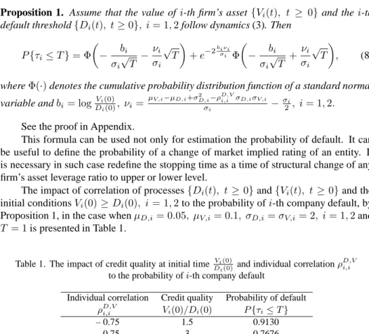
Proposition 1. Assume that the value ofi-th firm’s asset{Vi(t), t ≥ 0} and thei-th default threshold{Di(t), t≥0}, i= 1,2follow dynamics (3). Then
P{τi≤T}= Φ − bi σi √ T − νi σi √ T +e−2biνiσi Φ − bi σi √ T + νi σi √ T , (8)
whereΦ(·)denotes the cumulative probability distribution function of a standard normal variable andbi= logDVii(0)(0), νi=
µV,i−µD,i+σD,i−2 ρD,Vi,i σD,iσV,i
σi −
σi
2, i= 1,2. See the proof in Appendix.
This formula can be used not only for estimation the probability of default. It can be useful to define the probability of a change of market implied rating of an entity. It is necessary in such case redefine the stopping time as a time of structural change of any firm’s asset leverage ratio to upper or lower level.
The impact of correlation of processes{Di(t), t≥0}and{Vi(t), t≥0}and the
initial conditionsVi(0)≥Di(0), i= 1,2to the probability ofi-th company default, by
Proposition 1, in the case whenµD,i= 0.05, µV,i= 0.1, σD,i=σV,i= 2, i= 1,2and T = 1is presented in Table 1.
Table 1. The impact of credit quality at initial time Vi(0)
Di(0) and individual correlationρ
D,V i,i
to the probability ofi-th company default
Individual correlation Credit quality Probability of default ρD,Vi,i Vi(0)/Di(0) P{τi≤T} – 0.75 1.5 0.9130 – 0.75 3 0.7676 – 0.75 5 0.6653 – 0.5 1.5 0.9061 – 0.5 3 0.7495 – 0.5 5 0.6402 – 0.25 1.5 0.8971 – 0.25 3 0.7265 – 0.25 5 0.6085 0 1.5 0.8849 0 3 0.6956 0 5 0.5668 0.25 1.5 0.8671 0.25 3 0.6512 0.25 5 0.5082 0.5 1.5 0.8372 0.5 3 0.5795 0.5 5 0.4175 0.75 1.5 0.7704 0.75 3 0.4331 0.75 5 0.2515
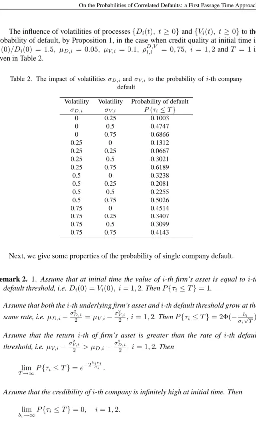
The influence of volatilities of processes{Di(t), t≥0}and{Vi(t), t ≥0}to the
probability of default, by Proposition 1, in the case when credit quality at initial time is
Vi(0)/Di(0) = 1.5, µD,i = 0.05, µV,i = 0.1, ρD,Vi,i = 0,75, i = 1,2andT = 1is
given in Table 2.
Table 2. The impact of volatilitiesσD,iandσV,i to the probability ofi-th company
default
Volatility Volatility Probability of default σD,i σV,i P{τi≤T} 0 0.25 0.1003 0 0.5 0.4747 0 0.75 0.6866 0.25 0 0.1312 0.25 0.25 0.0667 0.25 0.5 0.3021 0.25 0.75 0.6189 0.5 0 0.3238 0.5 0.25 0.2081 0.5 0.5 0.2255 0.5 0.75 0.5026 0.75 0 0.4514 0.75 0.25 0.3407 0.75 0.5 0.3099 0.75 0.75 0.4143
Next, we give some properties of the probability of single company default.
Remark 2. 1. Assume that at initial time the value ofi-th firm’s asset is equal toi-th default threshold, i.e.Di(0) =Vi(0), i= 1,2. ThenP{τi≤T}= 1.
2. Assume that both thei-th underlying firm’s asset andi-th default threshold grow at the same rate, i.e.µD,i−
σD,i2 2 =µV,i− σ2V,i 2 , i= 1,2. ThenP{τi ≤T}= 2Φ(− bi σi √ T).
3. Assume that the return i-th of firm’s asset is greater than the rate of i-th default threshold, i.e.µV,i−
σ2V,i 2 > µD,i− σ2D,i 2 , i= 1,2. Then lim T→∞P{τi≤T}=e −2biνiσi .
4. Assume that the credibility ofi-th company is infinitely high at initial time. Then
lim
5. lim σD,i→∞P{τi≤T}= Φ − √ T 2 +Di(0) Vi(0) Φ √ T 2 , i= 1,2. In addition, lim T→∞σD,i→∞lim P{τi≤T}= Di(0) Vi(0) , i= 1,2. 6. lim σV,i→∞P{τi ≤T}= Φ √ T 2 + Vi(0) Di(0) Φ − √ T 2 , i= 1,2. In addition, lim T→∞σV,i→∞lim P{τi≤T}= 1, i= 1,2.
Since the closed form expression of the probability of single default in case of stochastic default boundary is known, it’s sufficient to find the probabilityP{τ1≤T or
τ2≤T}orP{τ1≤Tandτ2≤T}.
5
Joint probability of correlated defaults
In this section, we investigate expression of the probabilityP{τ1≤T orτ2≤T}under the assumptions presented in Section 3.
Proposition 2. Assume that the value ofi-th firm’s asset{Vi(t), t≥ 0}and the value ofi-th default threshold{Di(t), t≥0}, i = 1,2follow dynamics (3). The cumulative distribution function of correlated default subject to initial conditionsVi(0) > Di(0), i= 1,2 is
P{τ1≤Torτ2≤T}
= 1−αT2 e−r 2 0
2Tea1d1+a2d2+a3T ∞ X n=1 sin nπθ 0 α Zα 0 sin nπθ α gn(θ)dθ, (9) where gn(θ) = ∞ Z 0 re−r 2 2T−c(θ)rInπ α rr0 T dr, Inπ α rr 0 T = ∞ X m=0 rr0 2T nπ α+2m m!Γ nπα +m+ 1
Euler’s gamma function, α= arctan − p 1−ρ2 ρ , if ρ <0, π+ arctan − p 1−ρ2 ρ , if ρ≥0, θ0= arctan b 2σ1 p 1−ρ2 −b1σ2+ρb2σ1 , if b 2σ1 p 1−ρ2 −b1σ2+ρb2σ1 >0 π+ arctan b2σ1 p 1−ρ2 −b1σ2+ρb2σ1 , if b2σ1 p 1−ρ2 −b1σ2+ρb2σ1 ≤0, a1= µD,1−µV,1−σ2D,1+ρ D,V 1,1 σD,1σV,1σ2 1−ρ2σ2 1σ2 − µD,2−µV,2−σ 2 D,2+ρD,V2,2 σD,2σV,2ρσ1 1−ρ2σ2 1σ2 , a2= µD,2−µV,2−σ2D,2+ρ D,V 2,2 σD,2σV,2σ1 1−ρ2σ2 2σ1 − µD,1−µV,1−σ 2 D,1+ρ D,V 1,1 σD,1σV,1 ρσ2 1−ρ2σ2 2σ1 , a3= a 2 1σ21 2 +ρa1a2σ1σ2+ a2 2σ22 2 −a1 µD,1−µV,1−σ 2 D,1+ρ D,V 1,1 σD,1σV,1 −a2 µD,2−µV,2−σD,2 2+ρD,V2,2 σD,2σV,2, c(θ) = b1 σ1sin(θ−α)− b2 σ2cos(θ−α), d1=a1σ1+ρa2σ2, d2=a2σ2 p 1−ρ2, r 0= b2 σ2sinθ0. See the proof in Appendix.
Remark 3. 1. Assume thatV2(0) =D2(0). ThenP{τ1≤Torτ2≤T}= 1.
2. It is natural that in the case of infinite maturity T, due to increasing uncertainty, the
joint probability of default approaches 1, i.e.:limT→∞P{τ1≤Torτ2≤T}= 1. 3. Assume thatθ0α is an integer4. ThenP{τ
1≤T orτ2≤T}= 1.
Corollary 1. The probability of both companies surviving is as follows:
P{τ1> T1andτ2> T2}= 1−P{τ1≤T1}−P{τ2≤T2}+P{τ1≤T1orτ2≤T2}.
4Such case is possible, for instance, if the coefficient of implied correlationρis negative, takingαclose to
Finally, knowing the default probability of each single company and the joint default probability of both firms, it is possible to calculate the default correlation. The implemen-tation of formula (9) is compuimplemen-tationally complicated because presented result requires double integration of nonlinear combination of modified Bessel function of the first kind. Also, the estimation of “implied” correlation needs to computationally estimate the vola-tilities and the correlations of Brownian motions{Vi(t), t ≥ 0}and{Di(t), t ≥ 0}, i = 1,2. On the other hand, it is clear that the given solution is not symmetric with respect to different defaults. So, the problem of selection of defaults arise, and it is not clear in what order select different defaults5.
Remark 4. Assume thatT1≤T2. Then
P{τ1≤T1orτ2≤T2}=P{τ1≤T1orτ2≤T1}+P{τ1≤T1andT1≤τ2≤T2}.
Remark 5. All the propositions in this paper are made for calculations at initial time t = 0. The same formulas hold in the case of anyt > 0. In such case, the constantT must be changed by the variableT−tfor anyt≥0and the default time ofi-th company, i= 1,2,τi= inf{t≥0 : Vi(t) =Di(t)}byτi= inf{s≥t: Vi(s) =Di(s)}.
6
Conclusion
The main result of this paper is the generalization of Zhou’s approach. The contribution of this paper is to derive analytical expression for the joint probabiloity of correlated defaults in the first passage time approach of credit risk which is necessary to quickly assess the credit risk of corporate bonds portfolio. The main assumptions in this paper are that both firm’s asset value and the default threshold follow geometric Brownian motions, i.e. by assuming stochastic behavior of default boundary, we also consider other exogenously defined type of financial risk, notably, liquidity and market changes risk and in such way expand credit risk modelling. On the other hand, one of the largest disadvantages of presented formulas of these formulas is the limited data for defining implied correlations, i.e., that its application requires a lot of aggregated information concerning secondary market of corporate bonds and the internal information about firm’s asset. In addition, the provided expression of joint probability of correlated defaults is not symmetric with respect to different company’s default.
The further step of this research could be the generalization of given formula of joint probability ofn >2correlated defaults. On the other hand, the generalization of probability of corporate bonds portfolio default in jump-diffusion case remains.
Appendix
Proof of Proposition 1. Using results of Zhou [1], where the default boundary follows
exponential function, i.e.Di(t) =Di(0)eµD,itthe probability of single company default
is given by P{τi≤T}= Φ − bi σV,i √ T − µV,i−µD,i σV,i √ T +e−2 (µD,i−µV,i)bi σ2V,i Φ − bi σV,i √ T + µV,i−µD,i σV,i √ T .
Assume that default boundary, (in special case, the value ofi-th bond) follows geomet-ric Brownian motion. Then after some simple calculations we have the expression of stopping time, i.e. the time when default of thei-th firm,i= 1,2occurs:
inf{t≥0 : Vi(t) =Di(t)}
= infnt≥0 :Vi(0)e µV,i−µD,i+σ 2
D,i−ρD,Vi,i σD,iσV,i− σ2i 2 t+σiWi(t)=D i(0) o . (10)
Let us define implied stochastic processes for anyt≥0by formulaYei(t) =Di(0)DVii((tt)),
e
Yi(0) =Vi(0), i = 1,2. Then we obtain implied geometric Brownian motions, for any t≥0described by equation
dYei(t) =Yei(t) (µi−µD,i)dt+σidWi(t), i= 1,2
with coefficients, defined in formula (6), and respective default thresholdsDi(0), and
unchanged initial conditions:Y˜i(0) =Vi(0)> Di(0), i= 1,2.
Let us rewrite the term in right-hand side in expression (10):
Vi(0)e µV,i−µD,i+σ 2
D,i−ρD,Vi,i σD,iσV,i− σ2i
2
t+σiWi(t)=V
i(0)eσiZi(t), i= 1,2.
whereZi(t) = νit+Wi(t), t ≥ 0,andνi = µi−σµiD,i − σ2i, i = 1,2.Hence, using the reflection principle for geometric Brownian motions (for more details, see [13]) the probability ofi-th firm default is given by
P{τi≤T}=P inf{t≥0 :Yei(t) =Di(0)} ≤T =P inf t≥0 :Zi(t) =− bi σi ≤T = 1−P mZi T ≥ − bi σi = Φ − bi σi √ T − νi σi √ T +e−2biνiσi Φ − bi σi √ T + νi σi √ T . wheremZi T = inf0≤t≤TZi(t), i= 1,2.
Proof of Proposition 2. Using the definition of default time of the i-th firm we have
P{τ1≤T orτ2≤T}. Technically, we calculate the probability
After some simple calculations we have the expression of stopping time, i.e. the time when default of thei-th firm occurs:
inf{t≥0 :Vi(t) =Di(t)}= inf
t≥0 :Vi(0)e µV,i+σ 2
D,i−ρD,Vi,i σD,iσV,i− σi2 2 t +σiWi(t) =Di(0)eµD,it , i= 1,2.
Let us define implied stochastic processes for anyt≥0by formula
Yi(t) =Di(0) Vi(t) Di(t)
eµD,it, Y
i(0) =Vi(0), i= 1,2.
Then we obtain implied geometric Brownian motions, described in formulas (5) and (6) for anyt≥0with correlation
ρ= Corr[logY1(t),logY2(t)] = Corr[W1(t), W2(t)].
The respective default thresholds areDi(0)eµD,itand the initial conditions left unchanged: Yi(0) =Vi(0)> Di(0), i= 1,2. Let us define Xi(t) =−log e−µD,itYi(t) Yi(0) , i= 1,2
that follows two-dimensional correlated arithmetic Brownian motion,
dX1(t) dX2(t) = λ1 λ2 dt−Θ dW1(t) dW2(t) , whereλi=µD,i−µi+σ 2 i
2 , i= 1,2andΘis a2×2covariance matrix such that
Θ·Θ′= σ2 1 ρσ1σ2 ρσ1σ2 σ22 ,
with the transformed initial conditionsXi(0) = 0andbi = logDVii(0)(0), i = 1,2. Let f(b1, b2, x1, x2, ρ, T) be the transition probability density of the particle in the region
{(x1, x2) : x1 < b1andx2< b2}before the maturityT. The finding of the probability
P{τ1≤Torτ2≤T}is equivalent to finding the first passage time ofXi(t)to a boundary bi, i= 1,2. Let us define the probability that the particle does not reach the fixed barrier ∂(b1, b2)in the time period[0, T], i.e.,
F(b1, b2, T) ≡PX1(T)< b1andX2(T)< b2| X1(s)< b1andX2(s)< b2, 0< s < T =P{τ1> T andτ2> T}= b1 Z −∞ b2 Z −∞ f(b1, b2, x1, x2, ρ, T)dx1dx2.
The problem of computing probability density is classical. It can be usually tackled using the separation of variables technique or more sophisticated methods such as contour integration and Laplace transform for the closely related problem of the solution of the heat equation on a wedge. Zhou [1], He, Keirstead and Rebholz [5] and Patras [7] followed the first approach. Patras analyzed the correlated default problem using planar Brownian motion constructions and its local isometry. Patras used this method in more general case, i.e. when induced by local (where local means with respect to time and space simultaneously) isometry from planar Brownian motion stochastic process behaves therefore locally as the usual planar Brownian motion and the subspace is only locally Euclidean. The transition probability density is the solution of Kolmogorov forward equation ∂f ∂T = σ2 1 2 ∂2f ∂x2 1 +ρσ1σ2 ∂ 2f ∂x1∂x2 +σ 2 2 2 ∂2f ∂x2 2 , x1< b1, x2< b2, (11) subject to the boundary conditions:
f(b1, b2,−∞, x2, ρ, T) =f(b1, b2, x1,−∞, ρ, T) = 0, f(b1, b2, x1, x2, ρ,0) =δ(x1)δ(x2), b1 Z −∞ b2 Z −∞ f(b1, b2, x1, x2, ρ, T)dx1dx2≤1, T >0, f(b1, b2, b1, x2, ρ, T) =f(b1, b2, x1, b2, ρ, T) = 0,
whereδ(x)is a Dirac’s Delta function and the equationf(b1, b2, x1, x2,0) =δ(x1)δ(x2) means the initial conditionXi(0) = 0, i = 1,2. The solution of Kolmogorov forward
equation subject to boundary conditions (for more details, see [5, 14] and [1]) for any fixedt >0is given by f(b1, b2, x1, x2, ρ, T) = 2 σ1σ2 p 1−ρ2αTe −r2 +r 2 0 2T ∞ X n=1 sin nπθ α sin nπθ0 α Inπ α rr0 T , (12) where x1=b1−σ1 p 1−ρ2rcosθ+ρrsinθ, x2=b2−σ2rsinθ.
The probability that the particle does not reach the barrier∂(b1, b2)during the period
[0, T]is given by F(b1, b2, T) = b1 Z −∞ b2 Z −∞ f(b1, b2, x1, x2, ρ, T)dx1dx2
= α Z 0 ∞ Z 0 rσ1σ2 p 1−ρ2f(α,∞, r, θ, ρ, T)dθdr = 2 αTe −r 2 0 2T ∞ X n=1 sin nπθ 0 α Zα 0 sin nπθ α dθ ∞ Z 0 re−r2 2TInπ α rr 0 T dr.
Hence, the probability of either company defaulting is as follows:
P{τ1≤T orτ2≤T}= 1−F(b1, b2, T) = 1−αT2 e−r 2 0 2T ∞ X n=1 sin nπθ 0 α Zα 0 sin nπθ α dθ ∞ Z 0 re−r 2 2TInπ α rr 0 T dr = 1−αT2 e−r 2 0
2Tea1d1+a2d2+a3T ∞ X n=1 sin nπθ 0 α Zα 0 sin nπθ α gn(θ)dθ. (13)
Acknowledgement
Thanks to Professor R. Leipus for valuable comments on this paper.
References
1. Ch. Zhou, An analysis of default correlations and multiple defaults, Review of Financial
Studies, 14(2), pp. 555–576, 2001.
2. K. Giesecke, Correlated defaults with incomplete information, Journal of Banking and
Finance, 28, pp. 1521–1545, 2004.
3. D. J. Lucas, Default correlation and credit analysis, Journal of Fixed Income, 4(4), pp. 76–87, 1995.
4. J.-P. Fouque, B. C. Wignall, X. Zhou, Modeling correlated defaults: first passage model under
stochastic volatility,http://www.defaultrisk.com/pp corr 89.htm.
5. H. He, W. P. Keirstead, J. Rebholz, Double lookbacks, Mathematical Finance, 8(3), pp. 201–228, 1998.
6. L. Overbeck, W. Schmidt, Modeling default dependence with threshold models, Journal of
Derivatives, 12(4), pp. 10–19, 2005.
7. F. Patras, A reflection principle for correlated defaults, Stochastic Processes and Their
Applications, 116, pp. 690–698, 2006.
8. L. Overbeck, G. Stahl, Stochastic essentials for the risk management of credit portfolios, Kredit
9. S. R. Das, G. Geng, Correlated default processes: a criterion-based copula approach, Journal
of Investment Management, 2(2), pp. 44–70, 2004.
10. K. Giesecke, L. R. Goldberg, A top down approach to multi-name credit, Working paper, Stanford University, 2007.
11. M. Davis, V. Lo, Modelling default correlation in bond portfolios, in: Mastering Risk II:
Applications, Carol Alexander (Ed.), Financial Times Prentice Hall, pp. 141–151, 2001.
12. H. Gersbach, A. Lipponer, Firm defaults and the correlation effects, European Financial
Management, 9(3), pp. 361–377, 2003.
13. M. Jeanblanc, Credit risk, M¨unich, 2002.
14. S. Iyengar, Hitting lines with two-dimensional Brownian motion, SIAM Journal of Applied
Mathematics, 45(6), pp. 983–989, 1985.
15. T. R. Bielecki, M. Rutkowski, Credit risk: modeling, valuation and hedging, Springer-Verlag, Berlin Heidelberg, 2004.
16. D. J. Duffie, K. J. Singleton, Simulating correlated defaults, Working Paper, Graduate School of Business, Stanford University, 1999.
17. I. S. Gradshteyn, I. M. Ryzhik, Table of integrals, series and products, New York, Academic Press, 1980.
18. J. Hull, A. White, Valuing credit default swaps II: modeling default correlations, Journal of