Identifying patterns in spatial
information: a survey of methods
Shashi Shekhar, Michael R. Evans, James M. Kang and
Pradeep Mohan
Explosive growth in geospatial data and the emergence of new spatial technolo-gies emphasize the need for automated discovery of spatial knowledge. Spatial data mining is the process of discovering interesting and previously unknown, but potentially useful patterns from large spatial databases. The complexity of spatial data and implicit spatial relationships limits the usefulness of conven-tional data mining techniques for extracting spatial patterns. In this paper, we explore the emerging field of spatial data mining, focusing on different methods to extract patterns from spatial information. We conclude with a look at future research needs.C 2011 John Wiley & Sons, Inc.WIREs Data Mining Knowl Discov2011 1 193–214 DOI: 10.1002/widm.25
INTRODUCTION
T
he significant growth of spatial data collection and widespread use of spatial databases1–4haveheightened the need for the automated discovery of spatial knowledge. Spatial data mining2,5 is the
pro-cess of discovering interesting and previously un-known, but potentially useful patterns from spatial databases. The complexity of spatial data and implicit spatial relationships limits the usefulness of conven-tional data mining techniques for extracting spatial patterns.
Specific features of geographical data that pre-clude the use of general purpose data mining algo-rithms are: (1) the spatial relationships among the variables; (2) the spatial structure of errors; (3) the presence of mixed distributions as opposed to com-monly assumed normal distributions; (4) observations that are not independent and identically distributed (i.i.d.); (5) spatial autocorrelation among the features; and (6) nonlinear interactions in feature space. Al-though conventional data mining algorithms can be applied under assumptions such as i.i.d., these algo-rithms often perform poorly on spatial data due to their self-correlated nature. To illustrate, we use an example from ecology where domain scientists are interested in studying the habitats of birds based on the attributes of locations in the study area, such as
∗Correspondence to: [email protected]
Department of Computer Science, University of Minnesota, Minneapolis, Minnesota, USA
DOI: 10.1002/widm.25
water depth. Figure 1 shows two different attributes, one with an assumption ofi.i.d. (Figure 1(a)) and one that has spatial autocorrelation (Figure 1(b)), that is, water depth in this case. Making use of water depth as an explanatory variable by accounting for spatial autocorrelation was found to model the ground truth better (i.e., predicting the habitat of birds).6
Efficient tools for extracting information from geospatial data are crucial to organizations that make decisions based on large spatial data sets. These application domains include public health,7–9
mapping and analysis for public safety,10
transpor-tation,11–14 environmental science and
manage-ment,15–19 economics,20 climatology,5,21,22 public
policy,23,24 earth science,25 market research and
analytics,26–28 public utilities and distribution,
etc.29–31 Many government and private agencies that
are likely beneficiaries of spatial data mining include the National Institute of Health (NIH), National In-stitute of Justice (NIJ), US Department of Trans-portation, (USDOT), US Department of Agriculture (USDA), National Aeronautics and Space Adminis-tration (NASA), National Oceanic and Atmospheric Administration (NOAA), IBM, and SIEMENS.
The challenges inherent in the management and analysis of spatial data sets have made spa-tial databases a particularly active area of research for several decades. The impacts of this research extend far and wide. To cite a few examples, the filter-and-refine technique used in spatial query pro-cessing has been applied to subsequence mining; multidimensional-index structures are used in com-puter graphics and image processing; and space-filling
F I G U R E 1|Attribute values in space with independent identical distribution and spatial autocorrelation. curves used in spatial query processing and data
storage are applied in dimension reduction prob-lems. The value of its contributions no longer in doubt, current research in spatial databases aims to improve its functionality, extensibility, and per-formance. The impetus for improving functional-ity comes from the needs of numerous existing ap-plications such as geographic information systems, location-based services,32and sensor networks.33
These research advances coupled with the grow-ing need for spatial information awareness have given rise to many commercial spatial database manage-ment systems (SDBMS). Some examples of SDBMS in-clude ESRI’s ArcGIS Geodatabase,34Oracle Spatial,35
IBM’s DB2 Spatial Extender and Spatial Datablade, and systems such as Microsoft’s SQL Server 2008.36
Spatial databases have played a major role in popular applications such as Google Earth37and Microsoft’s
Virtual Earth.38 Research prototype examples of
SDBMS include spatial datablades with PostGIS,39
MySQL’s Spatial Extensions,40Sky Server,41and
spa-tial extensions. The functionalities provided by these systems include use of spatial data types such as points, line segments and polygons, and spatial oper-ations such as inside, intersection, and distance. Spa-tial types and operations may be integrated into query languages such as SQL, which allows spatial query-ing to be combined with object-relational database management systems.42,43The performance
enhance-ment provided by these systems includes a multi-dimensional spatial index and algorithms for spatial database modeling such as OGIS44 and 3D
topo-logical modeling; spatial query processing including point, regional, range, and nearest neighbor queries;
and spatial data methods using a variety of indexes such as quad trees and grid cells.
In addition, there has been a growth in gen-eral purpose data mining tools such as Clementine from Statistical Package for the Social Sciences (SPSS), Enterprise Miner from SAS, Data Mining extensions from relational database vendors such as Oracle and IBM, public domain data mining packages such as Weka,45 See5/C5.0, etc., which are designed for the
purpose of analyzing data archived as transactions or other forms such as semi-structured data. Al-though these tools were primarily designed to identify customer-buying patterns in market basket data, they have also been used in analyzing scientific and en-gineering data, astronomical data, multi-media data, genomic data, and web data.46,47However, extracting
interesting and useful patterns from spatial data sets is more difficult than extracting corresponding patterns from traditional numeric and categorical data due to the complexity of spatial data types, spatial relation-ships, spatial autocorrelation, and nonlinearity.
The remainder of this paper is organized as follows: Spatial Data Inputs begins with a de-scription of the data input characteristics of sev-eral tasks in spatial data mining. Statistical Foun-dationsprovides an overview of the statistical foun-dation of spatial data mining (SDM). Spatial data mining tasks, explains in detail four main output patterns and methods of SDM related to anoma-lies, clustering, co-location, and prediction. Compu-tational issues regarding these patterns are discussed in Computational Issues. We survey some available spatial analysis tools for different SDM techniques in Spatial Analysis Tools. Future Directions and
Research Needsconcludes this paper with an exami-nation of research needs and future directions.
SPATIAL DATA INPUTS
The data inputs of SDM are more complex than the inputs of classical data mining because they include extended objects such as points, lines, and polygons in vector representation and field data in regular or irreg-ular tessellation such as raster data. The data inputs of SDM have two distinct types of attributes: nonspatial attributes and spatial attributes. Nonspatial attributes are used to characterize nonspatial features of objects such as name, population, and unemployment rate for a city. They are the same as the attributes used in the data inputs of classical data mining. Spatial attributes are used to define the spatial location and extent of spatial objects.48,49The spatial attributes of a spatial
object most often include information related to spa-tial locations, for example, longitude, latitude, and elevation, defined in a spatial reference frame, as well as shape.
In some applications, spatial data sets include discrete representations of continuous phenomena (e.g., ecology). Discretization of continuous space is necessitated by the nature of the digital represen-tation or semantics associated with the underlying phenomenon under study by an application domain. There are two basic models to represent spatial data, namely, raster (grid) and vector. Satellite images are good examples of raster data, while vector consists of points, lines, polygons, and their aggregate (or multi-) counterparts. This distinction is important because many of the techniques that we describe later favor one or more of these data types. Vector data over a space is a framework to formalize specific relation-ships among a set of objects. Depending on the re-lationships of interest, the space can be modeled in many different ways, that is, as set-based space, topo-logical space, Euclidean space, metric space, and net-work space.4 These models of space are described
briefly in this paper.
Set-based space uses the basic notion of ele-ments, element-equality, sets, and membership to for-malize set relationships such as set-equality, subset, union, cardinality, relation, function, and convexity. Relational and object-relational databases use this model of space.
Topological space uses the basic notion of a neighborhood and points to formalize extended ob-ject relations such as boundary, interior, open, closed, within, connected, and overlaps, which are invariant under elastic deformation. Combinatorial topological
space formalizes relationships such as Euler’s formula (number of faces+number of vertices−number of edges=2 for planar configuration). Network space is also a form of topological space in which the connec-tivity property among nodes formalizes graph proper-ties such as connectivity, isomorphism, shortest path, and planarity.
Euclidean coordinatized space uses the notion of a coordinate system to transform spatial proper-ties and relationships into properproper-ties of tuples of real numbers. Metric space formalizes distance relation-ships using positive symmetric functions that obey the triangle inequality. Many multidimensional applica-tions use Euclidean coordinatized space with metrics such as distance.
Apart from different concepts of space, many gazetteers employ spatial referencing with identifiers of a location that can be transformed into coordi-nates, such as a postal code (street addresses) or geo-name that is more natural to human understanding. Time is usually included in the spatial data as a time stamp.
During data input, relationships among non-spatial objects are made explicit through arith-metic relation, ordering, instance-of, subclass-of, and membership-of. In contrast, relationships among spa-tial objects are often implicit, such as overlap, inter-sect, and behind. Table 1 gives examples of spatial and nonspatial relationships. One possible way to deal with implicit spatial relationships is to materialize the relationships into traditional data input columns and then apply classical data mining techniques such as those described in Refs 50–54. However, the mate-rialization can result in loss of information. Usually, spatial and temporal vagueness, which naturally ex-ists in data and relationships, creates further model-ing and processmodel-ing difficulty in SDM. Another way
T A B L E 1 Common Relationships among Nonspatial and Spatial
Data
Nonspatial Relationship Spatial Relationship
Arithmetic Set-oriented: union, intersection, membership,. . .
Ordering Topological: meet, within, overlap,. . .
Is instance-of Directional: North, NE, left, above, behind,. . . Subclass-of Metric: e.g., distance, area,
perimeter,. . .
Part-of Dynamic: update, create, destroy,. . .
A B
C D
(a) Spatial framework
0 0 0 0 A B C D A B C D 1 1 0 1 1 0 0 0 0 0 1 1 1 0 0 A B C D A B C D 0.5 0.5 0.5 0.5 0.5 0.5 0.5 0.5 0 0 0 0 x i r t a m y t i u g i t n o C ) c ( p i h s n o i t a l e r r o b h g i e N ) b ( 1
F I G U R E 2|A spatial framework and its four-neighborhood contiguity matrix. to capture implicit spatial relationships is to develop
models or techniques to incorporate spatial informa-tion into the SDM process.
STATISTICAL FOUNDATIONS
Spatial statistics is a branch of statistics concerned with the analysis and modeling of spatial data.55
The field classifies spatial data into three basic types for ease of interpretation: (1) point referenced data, which is modeled as a fixed collection of spatial lo-cations, S, in a two-dimensional framework D (e.g., set of police stations in a metropolitan city); (2) areal data, modeled as a finite set of irregular shaped poly-gons in a two-dimensional framework D (e.g., set of police districts in a metropolitan city); and (3) point process data, which is modeled as a random collection of spatial events, collectively referred to as the spatial point pattern over a two-dimensional framework D (e.g., home locations of patients infected by a disease). In this section, three important statistical foundations are reviewed. They are: (1) spatial statistical interpre-tation models, (2) spatial neighborhood models, and (3) special properties of spatial data analysis.
Statistical interpretation models56are often used
to represent observations in terms of random vari-ables. These models can then be used for estimation, description, and prediction based on probability the-ory. Spatial data can be thought of as resulting from observations on the stochastic process Z(s) :s∈D, wheresis a spatial location andDis possibly a ran-dom set of points in a spatial framework. Three types of spatial statistical interpretation models that one might encounter are a point process, lattice, and geo-statistics.
Point process:A point process is a model for the spatial distribution of the points in a point pattern. Several natural processes can be modeled as spatial point patterns, for example, positions of trees in a
for-est and locations of bird habitats in a wetland. Spatial point patterns can be broadly grouped into random or nonrandom processes. Real point patterns are of-ten compared with random patterns (generated by a Poisson process) using the average distance between a point and its nearest neighbor.
Lattice:A lattice is a model for a gridded space in a spatial framework. Here, lattice refers to a count-able collection of regular or irregular spatial sites related to each other via a neighborhood relation-ship. Several spatial statistical analysis, for example, the spatial autoregressive model and Markov random fields, can be applied on lattice data.
Geostatistics:Geostatistics deals with the anal-ysis of spatial continuity and weak stationarity,56
which are inherent characteristics of spatial data sets. Geostatistics provides a set of statistics tools, such as kriging, to the interpolation of attributes at unsam-pled locations.
The spatial relationship among locations in a spatial framework is often modeled via a contigu-ity matrix. A simple contigucontigu-ity matrix may repre-sent a neighborhood relationship defined using ad-jacency or Euclidean distances. Example definitions of a neighborhood using adjacency include a four-neighborhood and an eight-four-neighborhood contiguity matrix.
Figure 2(a) shows a gridded spatial framework with four locations, A, B, C, and D. A binary ma-trix representation of a four-neighborhood relation-ship is shown in Figure 2(b). The row-normalized representation of this matrix is called a contiguity matrix, as shown in Figure 2(c). Other contiguity ma-trices can be designed to model neighborhood rela-tionship based on distance, different forms of con-nectivity (e.g., rook, queen), etc. The uniqueness of SDM originates from two central concepts in spatial statistics: spatial autocorrelation and spatial hetero-geneity(or nonstationarity).56–58
Spatial autocorrelation:One of the fundamental assumptions of traditional statistical analysis is that the data samples are independently generated: like successive tosses of coin or the rolling of a die. How-ever, in the analysis of spatial data, the assumption about the independence of samples is generally false. In fact, spatial data tend to be highly self-correlated. For example, people with similar characteristics, oc-cupation, and background tend to cluster together in the same neighborhoods. The economies of a re-gion tend to be similar. Changes in natural resources, wildlife, and temperature vary gradually over space. The property of like things clustering in space is so fundamental that geographers have elevated it to the status of the first law of geography: ‘Everything is re-lated to everything else, but nearby things are more related than distant things’.59 For example, Figure 1
shows the value distributions of an attribute in a spa-tial framework for an independent identical distribu-tion and a distribudistribu-tion with spatial autocorreladistribu-tion.
Spatial statistics has explored measures such as Ripley’s K Function, Spatial Scan Statistic, Moran’s I, Local Moran Index, Getis Ord, Geary’s C, etc. to quantify spatial correlation. These statistics have found many applications in common SDM tasks, in-cluding spatial co-location, spatial outlier detection, and hotspot discovery.
There is a strong relationship between measures of spatial autocorrelation and the contiguity matrix. This is because the contiguity matrix represents the relationship between a spatial unit and its neighbors. This neighborhood interaction is quantified by com-mon measures of spatial autocorrelation. However, the contiguity matrix for a particular spatial relation-ship may vary depending upon the definition of the spatial neighborhood. Such sensitivity in turn affects the robustness common measures of spatial autocor-relation (e.g., Moran’s I) and many spatial statistical models. This is a challenging problem due to the many possible methods of defining a spatial neighborhood, namely, graph based, grid based, etc. A detailed study of these challenges is beyond the scope of this paper.
Spatial heterogeneity: Apart from spatial auto-correlation, an important feature of spatial data sets is the variability of observed process over space. Spa-tial heterogeneity refers to the inherent variation in measurements of relationships over space. The influ-ence of spatial context on spatial relationships can be seen in the variation of human behavior over space (e.g., differing cultures). Different jurisdictions tend to produce different laws (e.g., speed limit differences between Minnesota and Wisconsin). The term spatial heterogeneity is most often used interchangeably with spatial nonstationarity, which is defined as the change
in the parameters of a statistical model or change in the ranking of candidate models over space.57
SPATIAL DATA MINING TASKS
Important tasks in SDM are spatial outlier detec-tion, co-location pattern discovery, spatial classifica-tion and regression modeling, spatial clustering, and spatial hotspot analysis. This section elaborates these techniques by briefly describing their computational structure, applications, and related methods.
Spatial Outlier Detection
Outliers have been informally defined as observations in a data set that appear to be inconsistent with the remainder of that set of data,60 or which
devi-ate so much from other observations as to arouse suspicions that they were generated by a different mechanism.61The identification of global outliers can
lead to the discovery of unexpected knowledge and has a number of practical applications in areas such as detection of credit card fraud and voting irregu-larities. This section focuses on spatial outliers, that is, observations that appear to be inconsistent with their neighborhoods.62–64Detecting spatial outliers is
useful in many geographic information systems and spatial databases applications such as transportation, ecology, homeland security, public health, climatol-ogy, and location-based services.
A spatial outlier65is a spatially referenced object
whose nonspatial attribute values differ significantly from those of other spatially referenced objects in its spatial neighborhood. Informally, a spatial outlier is a local instability (in values of non-spatial attributes) or a spatially referenced object whose nonspatial at-tributes are extreme relative to its neighbors, even though the attributes may not be significantly differ-ent from the differ-entire population. For example, a new house in an old neighborhood of a growing metropoli-tan area is a spatial outlier based on the nonspatial attribute house age.
Illustrative examples and application domains:
We use an example to illustrate the differences among global and spatial outlier detection methods. In Fig-ure 3(a), the X-axis is the location of data points in one-dimensional space; the Y-axis is the attribute value for each data point. Global outlier detection methods ignore the spatial location of each data point and fit the distribution model to the values of the nonspatial attribute. As shown in Figure 3(b), the outlier detected using this approach is the data point
G, which has an extremely high attribute value 7.9, exceeding the threshold ofμ+2σ =4.49+2∗
0 2 4 6 8 10 12 14 16 18 20 0 1 2 3 4 5 6 7 8 ← S P→ Q→ D↑ Original data points
Location Attr ib ute v alues Data point Fitting curve G L
(a) An example dataset
0 2 4 6 8 10 0 1 2 3 4 5 6 7 8 9
Histogram of attribute values
Attribute values
Number of occurrence
←
→ + 2
(b) Histogram F I G U R E 3|A data set for outlier detection.
1.61=7.71. This test assumes a normal distribution for attribute values. On the other hand,Sis a spatial outlier whose observed value is significantly different than its neighborsPandQ.
Common methods:Tests to detect spatial out-liers separate spatial attributes from nonspatial at-tributes. Spatial attributes are used to characterize location, neighborhood, and distance. Nonspatial at-tribute dimensions are used to compare a spatially referenced object to its neighbors. Spatial statistics literature provides two kinds of bi-partite multidi-mensional tests, namely, graphical tests and quanti-tative tests. Graphical tests, which are based on the visualization of spatial data, highlight spatial out-liers. Example methods include variogram clouds66
and Moran scatterplots.56,67 A variogram cloud
dis-plays data points related by neighborhood relation-ships. Figure 4(a) shows a variogram cloud for the example data set shown in Figure 3(a). This plot shows that two pairs (P,S) and (Q,S) on the left hand side lie above the main group of pairs and are possibly related to spatial outliers. A Moran scatter-plot shows the spatial association or disassociation of spatially close objects. The upper left and lower right quadrants of Figure 4(b) indicate a spatial association of dissimilar values: low values surrounded by high value neighbors (e.g., pointsPandQ) and high values surrounded by low values (e.g., pointS). Figure 4(b) indicates a spatial association of dissimilar values: low values surrounded by high value neighbors (e.g., pointsPandQ) and high values surrounded by low values (e.g., pointS).
A scatterplot68shows attribute values on theX
-axis and the average of the attribute values in the neighborhood on the Y-axis. A least square regres-sion line is used to identify spatial outliers. A scatter sloping upward to the right indicates a positive spatial autocorrelation (adjacent values tend to be similar); a scatter sloping upward to the left indicates a nega-tive spatial autocorrelation. The residual is defined as the vertical distance (Y-axis) between a point Pwith location (Xp,Yp) to the regression line Y=mX+b, that is, residual=Yp−(mXp+b). Cases with stan-dardized residualsstandard= −σμ greater than 3.0 or less than−3.0 are flagged as possible spatial outliers, whereμandσare the mean and standard deviation of the distribution of the error term, respectively. In Figure 5(a), a scatterplot shows the attribute values plotted against the average of the attribute values in neighboring areas for the data set in Figure 3(a). Point
Sturns out to be the farthest from the regression line and may be identified as a spatial outlier.
Spatial statistic S(x) is normally distributed if the attribute value f(x) is normally distributed. A popular test for detecting spatial outliers for nor-mally distributed f(x) can be described as follows: spatial statistic Zs(x)= |S(xσ)−sμs|> θ. For each
loca-tion, x with an attribute value f(x), the S(x) is the difference between the attribute value at location x
and the average attribute value ofxsneighbors,μs is the mean value ofS(x), andσsis the value of the stan-dard deviation ofS(x) over all stations. The choice of
θ depends on a specified confidence level. For exam-ple, a confidence level of 95% will lead toθ≈2.
0 0.5 1 1.5 2 2.5 3 3.5 0 0.5 1 1.5 2 2.5
Variogram cloud
Pairwise distanceSquare root of absolute diff
erence of attr ib ute v alues ← (Q,S) ← (P,S)
(a) Variogram cloud
0 0.5 1 1.5 2 2.5 0 1 2 3 S→ P→ Q→
Moran scatter plot
(b) Moran scatterplot v Z
F I G U R E 4|Variogram cloud and Moran scatterplot to detect spatial outliers.
1 2 3 4 5 6 7 8 2 2.5 3 3.5 4 4.5 5 5.5 6 6.5 7
Scatter plot
Attribute values A v er age attr ib ute v alues o v er neighborhood ← S P→ Q→ (a) Scatterplot 0 2 4 6 8 10 12 14 16 18 20 0 1 2 3 4Spatial statistic Zs(x) test
Location Zs(x) S→ P→ ← Q (b) Spatial statisticZs(x) F I G U R E 5|Scatterplot and spatial statisticZs(x)to detect spatial outliers.
Figure 5(b) shows the visualization of the spa-tial statistic method described above. The X-axis is the location of data points in one-dimensional space; the Y-axis is the value of spatial statistic Zs(x) for
each data point. We can easily observe that pointS
has a Zs(x) value exceeding 3 and will be detected
as a spatial outlier. Note that the two neighbor-ing points P and Q of S have Zs(x) values close to
−2 due to the presence of spatial outliers in their neighborhoods.
0 10 20 30 40 50 60 70 80 0 10 20 30 40 50 60 70 80 X Y s d
F I G U R E 6|Illustration of point spatial co-location patterns.
The techniques presented above are based on single attributes. However, multi-attribute based spa-tial outlier detection is also possible, such as with the average and median attribute value-based algorithms presented in Ref 69. Finally, we note that statistical tests used in outlier detection are normally prone to biases resulting from multiple hypothesis testing as spatial data sets are self-correlated. In order to deal with this, spatial statistics has explored several cor-rections to characterize the statistical significance of spatial outliers.67
Co-location Patterns
Co-location patterns represent subsets of boolean spa-tial features whose instances are often located in close geographic proximity. Examples include sym-biotic species and crime attractors (e.g., bars, mis-demeanors, etc.). Boolean spatial features describe the presence or absence of geographic object types at different locations in a two-dimensional or three-dimensional metric space, for example, the surface of the Earth. Examples of boolean spatial features in-clude plant species and crime.
Spatial co-location:Co-location rules are mod-els to infer the presence of boolean spatial features in
the neighborhood of instances of other boolean spa-tial features. For example, ‘Nile Crocodiles→ Egyp-tian Plover’ predicts the presence of EgypEgyp-tian Plover birds in areas with Nile Crocodiles. Figure 6 shows a data set consisting of instances of several boolean spatial features, each represented by a distinct shape. The shapes in Figure 6 represent different spatial fea-ture types. Spatial feafea-tures in sets{‘+’, ‘×’}and{‘o’, ‘∗’} tend to be located together. A careful review re-veals two co-location patterns, that is, (‘+’, ‘×’) and (‘o’, ‘∗’).
Co-location rule discovery is the process of iden-tifying co-location patterns from large spatial data sets with a large number of boolean features. The spatial co-location rule discovery problem looks sim-ilar to, but, in fact, is very different from the asso-ciation rule mining problem51because of the lack of
transactions. In market basket data sets, transactions represent sets of item types bought together by cus-tomers. The support of an association is defined to be the fraction of transactions containing the associ-ation. Association rules are derived from all the asso-ciations with support values larger than a user-given threshold.
Common methods:Spatial co-location rule min-ing approaches can be grouped into two broad
C2 C2 C2 C2 C2
Example dataset, neighboring instances of different features are connected B2 A1 A2 C1 B1 B2 A1 A2 C1 B1 Transactions{{B1},{B2}} support(A,B) = φ B2 Reference feature = C (b) A1 A2 C1 B1 B1
Support for (a,b) is order sensitive (c) 2 B 2 B (d) Support(A,B) = min(2/2,2/2) = 1 (a) B1 A1 C1 A2 Support(B,C) = min(2/2,2/2) = 1 A1 A2 C1 Support(A,B) = 1 Support(A,B) = 2
F I G U R E 7|Example to illustrate different approaches to discovering co-location patterns: (a) Example data set. (b) Reference feature-centric model. (c) Data partition approach. Support measure is ill-defined and order sensitive. (d) Event-centric model.
categories: approaches that use spatial statistics and algorithms that use association rule mining kind of primitives. Spatial statistics based approaches utilize statistical measures such as cross-K function, mean nearest-neighbor distance, and spatial autocorrela-tion. However, these approaches are computationally expensive. Association rule-based approaches focus on the creation of transactions over space so that an
a priorilike algorithm51can be used. Transactions in
space can use a reference-feature centric70approach
or a data-partition71approach. The reference-feature
centric model is based on the choice of a reference spatial feature70 and is relevant to application
do-mains focusing on a specific boolean spatial feature, for example, cancer. In the data partitioning ap-proach, transactions are created by making use of a prevalence measure that is order sensitive. In the spatial co-location rule mining problem, however, transactions are often not explicit. Force fitting the notion of transaction in acontinuous spatial frame-workwill lead to loss of implicit spatial relationships across the boundary of these transactions, as illus-trated in Figure 7. In the data set, in Figure 7(a), there are three feature types, A,B, and C, each of which has two instances. The neighbor relationships between instances are shown as edges. Co-locations (A,B) and (B,C) may be considered as frequent in this example. Figure 7(b) shows transactions created by choosingCas the reference feature. As Co-location (A,B) does not involve the reference feature, it will not be found. Figure 7(c) shows two possible parti-tions for the data set of Figure 7(a), along with the supports for co-location (A,B); in this case, the sup-port measure is order sensitive and may also miss the Co-location (A,B). However, the event-centric model addresses these limitations72 and finds
sub-sets of spatial features likely to occur in a neighbor-hood around instances of given subsets of event types (see Figure 7(d)).
Spatial Classification and
Regression Models
Spatial classification and regression models in data mining have been used to represent relationships be-tween variables in different data sets (e.g., climate). In most of these data sets, there are two sets of variables, namely, independent or explanatory variables and dependent variables. Although classification models deal with discrete values of dependent variables (e.g., class labels), regression models are concerned with continuous valued ones. In most SDM applications, classification and regression models can be learned from data in different ways such as supervised ing, unsupervised learning, and semi-supervised learn-ing. In this paper, we review only supervised learnlearn-ing. Given a sample set of input–output pairs, the objec-tive of supervised learning is to learn a function that matches reasonably well with the input data and pre-dicts an output for any unseen input (but assumed to be generated from the same distribution), such that the predicted output is as close as possible to the desired output. For example, in remote sensing im-age classification, the input attribute space consists of various spectral bands or channels (e.g., blue, green, red, infra-red, thermal, etc.) The input vectors (xi’s) are reflectance values at theithlocation in the image, and the outputs (yi’s) are thematic classes such as for-est, urban, water, and agriculture. The type of output attribute determines the supervised learning task; two such tasks are:
• Classification:Here, the input vectorsxi are assigned to a few discrete numbers of classes, for example, image classification73y
i.
• Regression:In regression, also known as func-tion approximafunc-tion or predicfunc-tion, the input– output pairs are generated from an unknown function of the form y= f(x), where y is
A
= Nest location
P = Predicted nest in pixel A = Actual nest in pixel
P P A A P P A A A (a) A A A (b) (c) (d) P P Legend
F I G U R E 8|(a) The actual locations of nests. (b) Pixels with actual nests. (c) Location predicted by a model. (d) Location predicted by another model. Prediction (d) is spatially more accurate than (c).
continuous. Typically, regression is used in regression and estimation, for example, crop yield prediction,74 daily temperature
predic-tion, and market share estimation for a par-ticular product. Regression can also be used in inverse estimation, that is, given that we have an observed value ofy, we want to determine the correspondingxvalue.
However, while performing supervised learning, conventional data mining techniques perform poorly in identifying values of dependent variables due to two reasons. The first reason is because they ignore spatial autocorrelation and heterogeneity in the model building process. A second, more subtle but equally important reason is related to the choice of the objec-tive function to measure classification accuracy. For a two-class problem, the standard way to measure classification accuracy is to calculate the percentage of correctly classified objects. However, this measure may not be the most suitable in a spatial context. This is because the measure ofSpatial accuracy—how far the predictions are from the actuals—is important in some applications such as ecology due to the effects of the discretization of a continuous wetland into dis-crete pixels, as shown in Figure 8. Figure 8(a) shows the actual locations of nests and (b) shows the pixels with actual nests. Note the loss of information dur-ing the discretization of continuous space into pixels. Many nest locations barely fall within the pixels la-beled ‘A’ and are quite close to other blank pixels, which represent ‘no-nest’. Now consider two predic-tions shown in Figure 8(c) and (d). Domain scientists prefer prediction 8(d) over (c), as the predicted nest locations are closer on average to some actual nest locations. The classification accuracy measure cannot distinguish between 8(c) and (d), and a measure of spatial accuracy is needed to capture this preference.
Common methods:Several previous studies75,76
have shown that the modeling of spatial dependency (often called context) during the classification or re-gression process improves overall accuracy. Spatial context can be defined by the relationships between spatially adjacent spatial units in a small
neighbor-hood. An example spatial framework and its four-neighborhood contiguity matrix is shown in Figure 2. Three supervised learning techniques for classification and regression that model spatial dependency are: (1) Markov random field (MRF) based classifiers; (2) lo-gistic spatial autoregression (SAR) model; and (3) ge-ographically weighted regression (GWR).
Markov random field-based Bayesian classifiers:
Maximum likelihood classification (MLC) is one of the most widely used parametric and supervised clas-sification technique in the field of remote sensing.77,78
However, MLC is a per-pixel based classifier and as-sumes that samples arei.i.d. Ignoring spatial autocor-relation results insalt and pepperkind of noise in the classified images. One solution is to use MRF-based Bayesian classifiers79to model spatial context via the a priori term in Bayes’ rule. This uses a set of ran-dom variables whose interdependency relationship is represented by an undirected graph (i.e., a symmet-ric neighborhood matrix). A more detailed theoretical and experimental comparison of these two methods can be found in Ref 80.
Logistic spatial autoregressive model (SAR): Lo-gistic SAR decomposes a classifier ˆfCinto two steps, namely, spatial autoregression and logistic transfor-mation. Spatial dependencies are modeled using the framework of logistic regression analysis. In the spa-tial autoregression model, the spaspa-tial dependencies of the error term, or the dependent variable, are directly modeled in the regression equation.81If the dependent
valuesyiare related to each other, then the regression equation can be modified as:
y=ρWy+Xβ+. (1)
Here,Wis the neighborhood relationship con-tiguity matrix andρ is a parameter that reflects the strength of the spatial dependencies between the ele-ments of the dependent variable via the logistic func-tion for binary dependent variables.
One limitation of the SAR model is that, it does not account for the underlying spatial heteorgeneity that is natural in geographic spaces. Thus, in Eq. (1), the model parameter estimatesβand the model errors
(a) CSR p attern (b) Clustered p attern
F I G U R E 9|Complete spatial random (CSR) and spatially clustered patterns.
are assumed to be uniform throughout the entire geographic space. One proposed method to account for spatial variation in model parameters and errors is Geographically Weighted Regression(GWR).82,83
The regression equation shown for GWR, shown by Eq. (2), has the same structure as standard linear re-gression, with the exception that the parameters are spatially varying.
y=Xβ(s)+(s), (2) where β(s) and (s) represent the spatially varying parameters and the errors, respectively.
Spatial Clustering
Spatial clustering is a process of grouping a set of spatial objects into clusters so that objects within a cluster have high similarity in comparison to one an-other, but are dissimilar to objects in other clusters.
Spatial statistics, the standard against which spatial point patterns are often compared, is a com-pletely spatially point process, and departures indicate that the pattern is not completely spatially random. Complete spatial randomness (CSR)56is synonymous
with a homogeneous Poisson process, the patterns of which are independently and uniformly distributed over space, that is, the patterns are equally likely to occur anywhere and do not interact with each other. In contrast, a clustered pattern is distributed depen-dently and attractively in space.
An illustration of complete spatial random pat-terns and clustered patpat-terns is given in Figure 9, which shows realizations from a completely spatially ran-dom process and from a spatial cluster process, re-spectively (each conditioned to have 85 points in a unit square).
Illustrative examples and application domains:
Cluster analysis is used in many spatial and spatiotem-poral application domains such as remote sensing data analysis as a first step to determine the number and distribution of spectral classes, in epidemiology
for finding unusual groups of health-related events, and in detection of crime hot spots by police officers. Notice in Figure 9 (a) that the CSR pattern seems to exhibit some clustering. This is not an un-representative realization but illustrates a well-known property of homogeneous Poisson processes: event-to-nearest-event distances are proportional toχ2
2
ran-dom variables, whose densities have a substantial amount of probability near zero.56 True clustering,
by contrast, is shown in Figure 9(b).
Common methods: Data mining and Machine learning literature have explored a large number of clustering algorithms which compute the statistical significance of spatial clusters to ensure that they are not random. The multitude of clustering algorithms can be classified into several groups as follows:
(1) Hierarchical clustering methods start with all patterns as a single cluster and succes-sively perform splitting or merging until a stopping criterion is met. This results in a tree of clusters, calleddendograms. The den-dogram can be cut at different levels to yield desired clusters. Well-known hierarchi-cal clustering algorithms include balanced iterative reducing and clustering using hi-erarchies (BIRCH), clustering using inter-connectivity (Chameleon), clustering using representatives (CURE), and robust cluster-ing uscluster-ing links (ROCK). More discussion of these methods can be found in Refs 84–86. (2) Partitional clustering algorithms start with
each pattern as a single cluster and itera-tively reallocate data points to each clus-ter until a stopping criclus-terion is met. These methods tend to find clusters of spherical shape. K-Means and K-Medoids are com-monly used partitional algorithms. Squared error is the most frequently used criterion function in partitional clustering. The re-cent algorithms in this category include par-titioning around medoids (PAM), clustering large applications (CLARA), clustering large applications based on randomized search (CLARANS), and expectation-maximization (EM). Related papers include Refs 87 and 88.
(3) Density-based clustering algorithms try to find clusters based on the density of data points in a region. These algorithms treat clusters as dense regions of objects in the data space. The density-based clustering algorithms include density-based spatial
clustering of applications with noise (DB-SCAN), ordering points to identify clustering structure (OPTICS), and density-based clus-tering (DECODE). Related research is dis-cussed in Refs 90–94.
Spatial Hotspot Analysis
Hotspots are a special kind of clustered pattern. As in clustered patterns, objects in hotspot regions have high similarity in comparison to one another and are quite dissimilar to all the objects outside the hotspot. One important feature that distinguishes a hotspot from a general cluster is that the objects in the hotspot area are more active compared with all others (den-sity, appearance, etc.). Spatial correlation of the at-tribute values within a hotspot could be high and possibly drops dramatically at the boundary, whereas in traditional clustering, the attribute values within a cluster could bei.i.d. Hotspot discovery/detection in SDM is a process of identifying spatial regions where more events are likely to happen, or more objects are likely to appear, in comparison to other areas.
Hotspot detection is mainly used in the analy-sis of crime and disease data. Crime data analyanaly-sis95
aims at finding areas that have greater than average numbers of criminal or disorderly events, or areas where people have a higher than average risk of vic-timization. Figure 10 shows two types of hotspots, namely, point hotspots and area hotspots. The design of hotspot maps is primarily oriented toward aiding law enforcement to make appropriate placement of their resources for crime investigation. For example, Figure 10(b) shows locations of bars with seven differ-ent colors obtained by using LISA,67the red squares
in the center, and peripheries of the map show the high crime activity bars. Maps such as the ones shown in Figure 10(a) show specific bars or hotspots where an increased attention for crime mitigation is neces-sary. On the other hand, if an analyst was interested in the geographic distribution of a particular crime type (e.g., Vandalism) based on an underlying base-line variable, one can make use of techniques such as kernel density estimation that is a part of tools such as CrimeStat.96For example, Figure 10(b) shows the
hotspots of vandalism incidents from the same city; the red cells indicate areas where there is a signifi-cantly high clustering of vandalism reports and the blue cells indicate cells where there is a significantly low concentration of vandalism, and grey indicates the area where there is no significant concentration. This map leads one to understand that, there is a sig-nificant clustering of vandalism incidents in the center of the city around the downtown areas.
F I G U R E 1 0|Spatial crime hotspots from the city of Lincoln, NE89(Best viewed in color).
Hotspot analysis finds applications in cancer/ disease data analysis, hotspots of locations where disease are reported intensively are detected, which may indicate a potential breakout of this disease, or suggest an underlying cause of the disease. Other domains of application include transportation (to identify unusual rates of accidents along highways) and ecology(to conduct geoinformatic surveillance for geospatial hot-spot detection97).
Common methods:Many of the standard clus-tering algorithms have been adapted for spatial hotspot analysis. These include K-Means, hierarchi-cal clustering, etc. Many other methods such as STAC (spatio-temporal analysis of crime)96 and LISA
(lo-cal indicators of spatial association)67have been
T A B L E 2 Algorithmic Strategies for Classical versus Spatial Data Mining
Algorithmic strategies for Classical data mining spatial data mining Divide-and-conquer Space partitioning
Filter-and-refine Minimum-bounding rectangle (MBR) Predicate approximation
Ordering Plane sweeping, space filling curve Hierarchical structures Spatial index, tree matching Parameter estimation Parameter estimation with spatial
autocorrelation
mitigation. Spatial hotspot analysis methods of par-ticular utility in public health applications such as syn-dromic surveillance and outbreak detection have been proposed. These methods include various frequentist and Bayesian statistical measures such as the spatial scan statistic98,99and space-time scan statistic.100,101
COMPUTATIONAL ISSUES
The volume of data, the complexity of spatial data types and relationships, and the need to identify spa-tial autocorrelation pose numerous computational challenges to the SDM field. When designing SDM al-gorithms, one has to take into account considerations such as space partitioning, predicate approximation, multidimensional data structures, etc. Table 2 sum-marizes how these requirements are in contrast with with classical data mining. Computational issues may arise due to high dimensionality of the spatial data set, spatial join process required in co-location min-ing and spatial outlier detection, estimation of SAR model parameters in the presence of large neighbor-hood matrixW, etc.
To illustrate these computational challenges, we use the case study of parameter estimation for the SAR model. The massive sizes of geospatial data sets in many application domains make it important to de-velop scalable parameter estimation algorithms of the SAR model solutions for location prediction and clas-sification. As noted previously, many classical data mining algorithms, such as linear regression, assume that the learning samples are i.i.d. This assumption is violated in the case of spatial data due to spa-tial autocorrelation;81 in such cases, classical linear
regression yields a weak model with not only low prediction accuracy102,103 but also residual error
ex-hibiting spatial dependence. Modeling spatial depen-dencies improves overall classification and regression accuracies significantly.
However, estimation of SAR model parameters is computationally very expensive because of the need to compute the determinant of a large matrix in the likelihood function.104–108 The maximum likelihood
(ML) function for SAR parameter estimation contains two terms: a determinant term and anSSEterm (Eq. 3). The former involves computation of the determi-nant of a very large matrix, which is a well-known hard problem in numerical analysis. Estimating the parameters of a ML-based SAR model solution, the log-likelihood function can be constructed, as shown in Eq. (3). The estimation procedure involves compu-tation of the logarithm of the determinant (log-det) of a large matrix, that is, (I−ρW).
(ρ|y)= −2 n ln |I−ρW| log−det +ln((I−ρW)y)T(I−x(xTx)−1xT)T ×(I−x(xTx)−1xT)((I−ρW)y) SSE (3)
As a result, the exact SAR model parameter estima-tion for a very small 10,000-point spatial problem can take tens of thousands of minutes on common desk-top computers. Computation costs make it difficult to use SAR for important spatial problems that involve millions of points, despite its promise to improve pre-diction and classification accuracy. In the equation, yis the n-by-1 vector of observations on the depen-dent variable, wherenis the number of observation points;ρis the spatial autoregression parameter;Wis then-by-nneighborhood matrix that accounts for the spatial relationships (dependencies) among the spatial data;xis then-by-kmatrix of observations on the ex-planatory variable, wherekis the number of features; and β is a k-by-1 vector of regression coefficients. Spatial autocorrelation termρWyis added to the lin-ear regression model in order to model the strength of the spatial dependencies among the elements of the dependent variable,y. The computational bottleneck in accounting for spatial autocorrelation is to evaluate the log-det for large problem sizes. Research in SDM has explored both approximate and exact solutions to the SAR model.109
SPATIAL ANALYSIS TOOLS
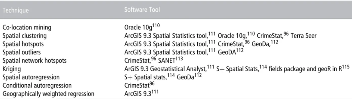
This section surveys currently existing spatial anal-ysis tools and presents a brief critique of the SDM functionalities they support. Spatial analysis methods including many of the SDM techniques, such as co-location mining, spatial hotspot analysis, and
T A B L E 3 Spatial Analysis Techniques in Popular Software
Technique Software Tool
Co-location mining Oracle 10g110
Spatial clustering ArcGIS 9.3 Spatial Statistics tool,111Oracle 10g,110CrimeStat,96Terra Seer Spatial hotspots ArcGIS 9.3 Spatial Statistics tool,111CrimeStat,96GeoDa,112
Spatial outliers ArcGIS 9.3 Spatial Statistics tool,111GeoDA112 Spatial network hotspots CrimeStat,96SANET113
Kriging ArGIS 9.3 Geostatistical Analyst,111S+Spatial Stats,114fields package and geoR in R115 Spatial autoregression S+Spatial stats,114GeoDa112
Conditional autoregression CrimeStat96
Geographically weighted regression ArcGIS 9.3111
geographically weighted regression, have found their way into commercial products such as Oracle,110
ArcGIS,111 TerraSeer, etc. Beyond these commercial
products, there are many public domain and open source tools such as GeoDA,112 CrimeStat,96 and
many libraries in R115 that provide useful
function-alities for performing spatial autoregression, kriging, and techniques for measuring spatial autocorrelation. Table 3 lists different spatial analysis methods and various tools supporting them.
Many of the above listed tools offer functional-ities to perform rigorous significance testing of SDM tools except commercial databases such as Oracle 10g. Added to this, many of the above tools sup-port exploratory analysis with visualization using an interactive display. Despite their usefulness in many applications, tools such as CrimeStat and Oracle 10g are limited in their capabilities to provide interactive map based visualization of results.
FUTURE DIRECTIONS AND
RESEARCH NEEDS
This section presents future directions and research needs in SDM. There are several new areas of re-search, but the two we will focus on are network-based SDM and spatio-temporal data mining.
Network Patterns
Many spatial phenomena such as distribution of crimes and distribution of accidents in large cities may be constrained by the transportation network struc-ture. One of the main challenges in SDM is to account for the network structure in the data set. For exam-ple, in hotspot detection, spatial techniques do not consider the spatial network structure of the data set, that is, they may not be able to model graph prop-erties such as one-ways, connectivities, left-turns, etc.
In this section, we present Spatial network activity hotspots, an interesting SDM problem that has a spa-tial network as a part of its input.
Spatial network activity hotspots: The prob-lem of identifying Spatial network hotspots(SNAH) is to discover those connected subsets of a spatial net-work whose attribute values are significantly higher than expected (Figure 11(b)). Finding SNAH is par-ticularly important for crime analysis (high-crime-density street discovery) and law enforcement (plan-ning effective and efficient patrolling strategies). In ur-ban areas, many human activities are centered about spatial infrastructure networks, such as roads and highways, oil/gas pipelines, and utilities (e.g., wa-ter, electricity, telephone). Thus, activity reports such as crime logs may often use network-based location references (e.g., street addresses). In addition, spa-tial interaction among activities at nearby locations may be constrained by network connectivity and net-work distances (e.g., shortest paths along roads or train networks) rather than the geometric distances used in traditional spatial analysis. Traditional meth-ods that employ a geometric summarization scheme to identify concentrations of crime may not account for large crime concentrations that are normally ac-counted for by the network-based methods. For ex-ample, Figure 11(a) and (b) show a comparison be-tween an ellipse-based geometric hotspot method and a network-based hotspot method for a data set from the recent Haiti earthquake. Crime prevention may focus on identifying subsets of ST networks with high activity levels, understanding underlying causes in terms of network properties, and designing network control policies. Identifying and quantifying SNAH
is a challenging task due to the need to choose the correct statistical model. In addition, the discovery process in large spatial networks is computationally very expensive due to the difficulty of characterizing and enumerating the population of streets to define
1 2 3 4 5 6 t = 20 20 20 20 20 20 20 40 20 40 20 20 1 1 1 1 1 1 7 8 9 10 20 20 20 20 40 20 40 40 Up = Down = TT = 1 1 1 1
(a) Example i nput
1 2 3 4 5 6 t = 20 20 20 20 20 20 20 40 20 40 20 20 1 1 1 1 1 1 7 8 9 10 20 20 20 20 40 20 40 40 Up = Down = TT = 1 1 1 1 (b) Example output
F I G U R E 1 2|Flow anomaly example.
a normal or expected activity level. Preliminary ex-ploration of descriptive and explanatory models for network patterns is available in Ref 116. However, further challenges and research is needed to identify other interesting patterns within network data sets, such as partial segments of roads that are more inter-esting than other parts.
Spatio-temporal Data Mining
Spatio-temporal data are often modeled using events and processes, both of which generally represent change of some kind. Processes refer to ongoing phe-nomena that represent activities of one or more types without a specified endpoint.117–119 Events refer to
individual occurrences of a process with a specified beginning and end. Event-types and event-instances are distinguished. For example, a hurricane event-type may occur at many different locations and times, for example, Katrina (New Orleans, 2005) and Rita (Houston, 2005). Each event-instance is associated with a particular occurrence time and location. The ordering may be total if event-instances have disjoint occurrence times. Otherwise, ordering is based on spatio-temporal semantics such as partial order, and spatio-temporal patterns can be modeled as partially ordered subsets. These unique characteristics create new and interesting challenges for discovering spatio-temporal patterns. For example, in contrast to spatial outliers, a spatio-temporal outlier is a spatio-temporal object whose thematic (nonspatial and nontempo-ral) attributes are significantly different from those of other objects in its spatial and temporal neighbor-hoods. A spatio-temporal object is defined as a time-evolving spatial object whose evolution or history is represented by a set of instances (EQ), where the space stamp is the location of the objectoid at timestamp
t. In the remainder of this section, we present re-search trends in various areas of spatio-temporal data mining.
Flow anomalies: Given a percentage threshold and a set of observations across multiple spatial loca-tions, flow anomaly discovery aims to identify domi-nant time intervals where the fraction of time instants
of significantly mismatched sensor readings exceeds a given percentage threshold. Figure 12 gives a simple example of flow anomalies (FAs). In Figure 12(a), the input to the FA problem consists of two spatial loca-tions [i.e., an upstream (up) and downstream (down) sensor], 10 time instants, and the notion of travel time (TT) or flow between the locations. For simplic-ity, the TT is set to a constant of 1, but it can be a variable. The output contains two FAs; using the time instants at the upstream sensor, periods 1–3 and 6–9, where the majority of time points show signif-icant differences in between (Figure 12(b)). Discov-ering FAs is important for water treatment systems, transportation networks, and video surveillance sys-tems. However, mining FAs is computationally ex-pensive due to the large (potentially infinite) num-ber of time instants across a spatial network of lo-cations. Traditional outlier detection methods (e.g.
t-test) are suited for detecting transient FAs (i.e., time instants of significant mismatches across consecutive sensors) but cannot detect persistent FAs (i.e., long variable time windows with a high fraction of time instant transient FAs) due to lack of a predetermined window size. Spatial outlier detection techniques do not consider the flow (i.e., TT) between spatial lo-cations and cannot detect any type of FAs. Prelimi-nary work introduced a time-scalable technique called SWEET (Smart Window Enumeration and Evalua-tion of persistent-Thresholds) that utilizes several al-gebraic properties in the flow anomaly problem to discover these patterns efficiently.120–122 However,
further research is needed to discover other types of patterns within this environment. In the context of transportation networks, researchers proposed simi-lar ST outlier patterns for identifying traffic accidents known as anomalous window discovery.123–125
Teleconnected flow anomalies: An additional pattern that utilizes FAs is teleconnected patterns.126
A teleconnection represents a strong interaction be-tween paired events that are spatially distant from each other. Identifying teleconnected flow events is computationally hard due to the large number of time instants of measurement, sensors, and locations. For
example, a well-known teleconnected event pair in-volves the warming of the eastern pacific region (i.e., El Nino) and unusual weather patterns throughout the world.127 Recently, a RAD (Relationship
Anal-ysis of Dynamic-neighborhoods) technique has been proposed that models flow networks to identify tele-connected events.126Further research is needed to
ex-plore new and interesting patterns that may lie within the RAD model.
Mixed-drove co-occurrence patterns: Another type of dynamic behavior of spatial data sets that might affect co-location patterns is changing the spec-ification of zone of interest and measuring values according to user preferences. Mixed-drove spatio-temporal co-occurrence patterns (MDCOPs) repre-sent subsets of two or more different object-types whose instances are often located in spatial and tem-poral proximity. Discovering MDCOPs is potentially useful in identifying tactics in battlefields and games, understanding predator–prey interactions, and in transportation (road and network) planning.128,129
However, mining MDCOPs is computationally very expensive because the interest measures are compu-tationally complex, data sets are larger due to the archival history, and the set of candidate patterns is exponential in the number of object-types. Prelimi-nary work has produced a monotonic composite in-terest measure for discovering MDCOPs and novel MDCOP mining algorithms.130
Cascading spatio-temporal patterns Partially ordered subsets of event-types whose instances are lo-cated together and occur in stages are called cascading spatio-temporal patterns (CSTP).131 Figure 13 shows
some interesting partially ordered patterns that were discovered from real spatio-temporal crime data sets from the city of Lincoln, Nebraska.89In the domain of
public safety, events such as bar closings and football games are considered generators of crime. Preliminary analysis revealed that football games and bar closing events do indeed generate CSTPs. CSTP discovery can play an important role in disaster planning, climate change science132,133 (e.g., understanding the effects
of climate change and global warming), and public health (e.g., tracking the emergence, spread, and re-emergence of multiple infectious diseases134). Further
Increase (larceny, v andalism, assaults) Increase (larceny, v andalism, assaults)
Bar closing (Saturday night)
Increase (larceny, v andalism, assaults)
Football night Football night Saturday night
F I G U R E 1 3|Cascading spatio-temporal patterns from public safety.
research is needed, however, to deal with challenges such as the lack of computationally efficient, statisti-cally meaningful metrics to quantify interestingness, and the large cardinality of candidate pattern sets that are exponential in the number of event types. Exist-ing literature for spatio-temporal data minExist-ing focuses on mining totally ordered sequences or unordered subsets.135–137
Broader Future Directions
In this paper, we have presented the major research achievements and techniques that have emerged from SDM, especially for predicting locations and discov-ering spatial outliers, co-location rules, and spatial clusters. Current research is mostly concentrated on developing algorithms that model spatial and spatio-temporal autocorrelations and constraints. Spatio-temporal data mining remains, however, still largely an unexplored territory; thus, we conclude by noting other areas of research that require further investiga-tion, such as the mining of movement data involv-ing groups of people, ideas, goods, and streaminvolv-ing data. Any SDM method is influenced by the neigh-borhood method selected. Hence, new computational algorithms and interest measures that deal with the sensitivity to spatial neighborhood size need to be de-fined. Most urgently, methods are needed to validate the hypotheses generated by SDM algorithms as well as to ensure that the knowledge generated is action-able in the real world.
ACKNOWLEDGEMENTS
We are particularly grateful to our collaborators Prof. Vipin Kumar, Prof. Paul Schrater, Prof. Sanjay Chawla, Dr. Chang-Tien Lu, Dr. Weili Wu, and Prof. Uygar Ozesmi, Prof. Yan Huang,
and Dr. Pusheng Zhang for their various contributions. We are particularly grateful to Dev Oliver, Xun Zhou, and Zhe Jiang for their feedback and help in preparing this paper. We also thank Prof. Hui Xiong, Prof. Jin Soung Yoo, Dr. Baris Kazar, Prof. Mete Celik, Dr. Betsy George, Dr. R.R Vatsavai and anonymous reviewers for their valuable feedback on early versions of this paper. We would like to thank Kim Koffolt for improving the readability of this paper.
REFERENCES
1. G ¨uting R. An Introduction to Spatial Database Sys-tems. In: Schek HJ, ed.VLDB Journal. London, UK: Springer-Verlag; 1994, 3:357–399.
2. Shekhar S, Chawla S. Spatial databases: A tour. Pren-tice Hall. NJ, USA: Upper Saddle River; 2002. ISBN: 0-7484-0064-6.
3. Shekhar S, Chawla S, Ravada S, Fetterer A, Liu X, Lu C-T. Spatial Databases - Accomplishments and Research Needs.Trans. on Knowledge and Data En-gineering1999, 11:45–55.
4. Worboys M, Duckham M.GIS: A Computing Per-spective. Second Edition. Boca Raton, FL, USA: CRC Press; 2004. ISBN: 978-0415283755.
5. Stolorz P, Nakamura H, Mesrobian E, Muntz R, Shek E, Santos J, Yi J, Ng K, Chien S, Mechoso R, Farrara J. Fast Spatio-Temporal Data Mining of Large Geophysical Datasets. In: Proceedings of the First International Conference on Knowledge Discov-ery and Data Mining. Menlo Park, CA, USA: AAAI Press; 1995, 300–305.
6. Chawla S, Shekhar S, Wu W-L, Ozesmi U. Model-ing spatial dependencies for minModel-ing geospatial data. In:ACM SIGMOD Workshop on Research Issues in Data Mining and Knowledge Discovery 2000, 70– 77.
7. Albert P, McShane L. A generalized estimating equa-tions approach for spatially correlated binary data: Applications to the analysis of neuroimaging data.
Biometrics1995, 51:627–638.
8. Cromley E, McLafferty S.GIS and public health. The Guilford Press, 2002.
9. Elliott P, Wakefield J, Best N, Briggs D.Spatial Epi-demiology: Methods and Applications. Oxford Uni-versity Press, 2000. ISBN: 978-0192629418. 10. Eck JE, Chainey S, Cameron JG, Leitner M, Wilson
RE. Mapping Crime: Understanding Hot Spots. Na-tional Insitute of Justice (NIJ) Special Report NCJ 209393, U.S. Department of Justice, Washington D.C., USA.
11. Lang L. Transportation GIS. Redlands, CA, USA: ESRI Press; 1999. ISBN: 978-1879102471.
12. Leipnik MR, Albert DP. GIS in Law Enforcement: Implementation Issues and Case Studies. London/
New York: CRC Press; 2002. ISBN:
978-0415286107.
13. Shekhar S, Yang T, Hancock P. An Intelligent Vehi-cle Highway Information Management System. Intl
J Microcomputers in Civil Engineering. New York: John Wiley & Sons; 1993, 8.
14. Thill J. Geographic information systems for trans-portation in perspective. Transportation Research Part C: Emerging Technologies2000, 8:3–12. 15. Issaks E, Svivastava M. Applied Geostatistics.
Ox-ford: Oxford University Press; 1989.
16. Kanevski M, Parkin R, Pozdnukhov A, Timonin V, Maignan M, Demyanov V, Canu S. Environmental data mining and modeling based on machine learn-ing algorithms and geostatistics.Environmental Mod-elling & Software2004, 19:845–855.
17. Haining RJ.Spatial Data Analysis in the Social and Environmental Sciences. Cambridge: Cambridge Uni-versity Press; 1989.
18. Roddick J-F, Spiliopoulou M. A Bibliography of Temporal, Spatial and Spatio-Temporal Data Min-ing Research. SIGKDD Explorations 1999, 1:34– 38.
19. Scally R.GIS for Environmental Management. Red-lands, CA, USA: ESRI Press; 2006. ISBN: 978-589481429.
20. Krugman P. Development, Geography, and Eco-nomic Theory. Cambridge, MA: MIT Press; 1995. 21. Ganguly A, Steinhaeuser K. Data mining for climate
change and impacts. In:IEEE International Confer-ence on Data Mining Workshops, 2008. ICDMW’08
2008, 385–394.
22. Yasui Y, Lele S. A regression method for spatial dis-ease rates: An estimating function approach. J Am Stat Assoc1997, 94:21–32.
23. Calkins H. GIS and public policy.Geographical In-formation Systems1990, 2:233–245.
24. Greene R.GIS in public policy: Using geographic in-formation for more effective government. Radlands, CA, USA: ESRI Press, 2000. ISBN: 978-1879102668. 25. Hohn M, Liebhold LGAE. A Geostatistical model for Forecasting the Spatial Dynamics of Defoliation caused by the Gypsy Moth, Lymantria dispar (Lep-idoptera:Lymantriidae).Environmental Entomology (Publisher: Entomological Society of America)1993, 22:1066–1075.
26. Maguire D. Implementing spatial analysis and GIS applications for business and service planning. In: Longley PA, Clarke G, eds.GIS for Business and Ser-vice Planning. New York: John Wiley & Sons; 1995, 171–191. ISBN: 978-0470235102.