Contents lists available atScienceDirect
Journal of Multivariate Analysis
journal homepage:www.elsevier.com/locate/jmva
Semiparametric analysis of longitudinal zero-inflated count data
Jiarui Feng, Zhongyi Zhu
∗Department of Statistics, Fudan University, Shanghai, 200433, PR China
a r t i c l e i n f o
Article history:
Received 24 January 2010 Available online 12 August 2010 AMS subject classifications: 62G20 62F12 62G08 Keywords: ZIP regression Mixed model Penalized spline MCEM algorithm
a b s t r a c t
In this article, we consider a semiparametric zero-inflated Poisson mixed model that postulates a possible nonlinear relationship between the natural logarithm of the mean of the counts and a particular covariate in the longitudinal studies. A penalized log-likelihood function is proposed and Monte Carlo expectation–maximization algorithm is used to derive the estimates. Under some mild conditions, we establish the consistency and asymptotic normality of the resulting estimators. Simulation studies are carried out to investigate the finite sample performance of the proposed method. For illustration purposes, the method is applied to a data set from a pharmaceutical company where the variable of interest is the number of episodes of side effects after the patient has taken the treatments.
©2010 Elsevier Inc. All rights reserved.
1. Introduction
Zero-inflated count data occurs in many areas such as public health, epidemiology, medicine, engineering and ecology. The most marked feature of this kind of data is that the number of zeros is much more than the one some common distributions for count data can predict. A two state process is often used to describe the generation of such data. One is called the zero state, in which the value of the observation can only be zero. In the other state, the observations can be generated from common distributions, such as Poisson distribution. In detail, we suppose the random variable is sampled from a degenerate distribution at zero with probabilitypand sampled from a Poisson (
µ
) distribution with probability 1−
p. We call it the zero-inflated Poisson (ZIP) model. Cohen [5], Johnsen and Kotz [10] discussed the ZIP models without covariates. Lambert [11] analyzed the number of defects in a manufacturing process and first applied the ZIP model in a regression set up. After that, ZIP regression has been widely used in various areas. Welsh et al. [23] examined the living conditions of rare species. Shankar et al. [21] modeled the accident frequencies. Bohning et al. [2] investigated the data from the study of prevention in dental epidemiology. Cheung [3] presented a detailed analysis about children’s growth and development in a medical survey.Because of longitudinal or hierarchical study design or data collection, longitudinal or clustered zero-inflated count data often occurs in public health surveys, medical trials and insurance. Ignoring the within-cluster correlation will lead to the loss of efficiency and the incorrect inference of the regression coefficients. To accommodate the features of longitudinal studies, many authors introduce two common methods, the marginal model and the conditional model, to ZIP regression. Dobbie and Welsh [6] employed the marginal ZIP regression by the GEE method [13]. Hall and Zhang [8] applied the GEE method to the EM algorithm, and proposed the expectation solution(ES) algorithm to estimate the unknown parameters in ZIP regression. Another popular way to analyze such data is the ZIP mixed model. Hall [7] considered the ZIP and ZIB regression models with the random intercept and proposed the EM algorithm. Wang et al. [22] obtained the penalized likelihood function by regarding random effects as the unknown parameters and use REML method for estimation. Xie et al. [24] analyzed the number of days of psychiatric hospitalization by ZIP mixed model.
∗Corresponding author.
E-mail address:[email protected](Z. Zhu).
0047-259X/$ – see front matter©2010 Elsevier Inc. All rights reserved. doi:10.1016/j.jmva.2010.08.001
In longitudinal data, the effect of some continuous covariates, such as time, age, may not be linearly related to the link function. Artificial assumption of their relationship may lead to model misspecification. Nonparametric methods are extremely useful to overcome this shortcoming. We can explore the potential nonlinear effect of the time on the response without any assumption. This is a natural approach to employ the semiparametric extension of ZIP regression model. Barry and Welsh [1] discussed the generalized additive model for zero-inflated count data. But they only fitted the truncated Poisson and negative binomial model and did not consider the ZIP regression. Lam et al. [12] constructed the semiparametric ZIP regression by Sieve MLE. Piecewise linear function was used to approximate the unknown smooth function. And the asymptotic properties were also discussed in the paper. For longitudinal or clustered zero-inflated data, their model can be easily extended, but the properties of the estimator were difficult to derive. Chiogna and Gaetan [4] applied the semiparametric ZIP models to animal abundance study. They used the penalized splines as the approximation of the smooth function and estimated the parameters via an EM algorithm. The variances of the estimators can be calculated by the Hessian matrix of the penalized log-likelihood function. But they focused on the application in the ecology research and skip the properties of the estimators. Moreover, ecological researches are usually conducted by areas so that data may show intra-area correlation, which was not considered in the paper either.
The work in this article is motivated by data from an experiment of a pharmaceutical company. One aspect of this experiment is to compare two treatments for a particular disease in terms of the number of episodes of a certain side effect. How to decrease the occurrence of the side effect is very important to both the company and the patients. Because of the large proportion of zeros, ZIP regression is used to analyze the effect of some covariates on the response. Min and Agresti [16] analyzed this data set by assuming the linear effect of natural logarithm of the exposure time-between-visits on the link function of the Poisson regression through a zero-altered mixed model. The results from their study provided the information that the time-between-visits had little effect on the numbers of side effects. However, the assumption of the monotonic trend seem to be inappropriate, mainly because the time effects may be very different when the lengths of the exposure time vary.
Our goal in this paper is to develop a semiparametric ZIP mixed model (SZIPMM) to explore the nonlinear effects of some continuous covariates on the response under the framework of longitudinal studies. The aforementioned models only focused on one aspect of the problem. The difficulty in developing the estimation procedures of SZIPMM is due to the fact that the objective function needed to be optimized is more complicated than the one under the parametric framework. Our approach is an extension of Hall’s [7] model and method. A smooth function and a random intercept are added to the Poisson regression. Penalized splines are used to approximate the smooth function and a penalized log-likelihood function is also obtained. The GCV method proposed by Qu and Li [18] is employed here to choose the smoothing parameter. We accommodate Hall’s [7] method roughly to obtain the likelihood function and propose our estimation procedures. The complexity of the integral determining the likelihood function depends on the random effect structure. As in the one-dimensional integral for the model proposed by Hall [7], the Gauss quadrature method was used to approximate the likelihood function. However, when the dimension of the integral grows higher, it is very difficult to achieve adequate approximation. Then Monte Carlo method is a good alternative to handle multivariate random effects. In this paper, we apply the McCulloch’s [15] MCEM approach, which makes our algorithm more flexible. Lambert [11] proved the asymptotic properties of the ZIP regression for the cross-sectional data. But in the longitudinal study, the large sample theory has not been discussed yet. We prove the consistency and the asymptotic normality of the estimators in the mild condition. And the asymptotic variance is obtained by the Sandwich formula.
This article is organized as follows: In Section2, we present the semiparametric ZIP mixed model and propose the estimation procedure. In Section3, we establish the consistency and asymptotic normality of the proposed estimators. We assess the finite sample performance of the proposed estimators with a Monte Carlo simulation in Section4. In Section5, we illustrate the method of this paper by a real data set. A brief summary and further discussion are given in Section6.
2. Models and MCEM algorithm
2.1. Semiparametric ZIP mixed model (SZIPMM)
Suppose the response vectorY contains data fromKindependent subjects so thatY
=
(
Y1T, . . . ,
YKT)
T, whereY i=
(
Yi1, . . . ,
YiTi)
T. We assume that, conditional on a random effectb
i,Yijfollows a zero-inflated Poisson distribution, i.e.Yijis generated from a two-state process. With probabilitypij, the first state, called the zero state, occurs, where no events are observed. With probability 1
−
pij,Yijfollows a standard Poisson distribution, which we call the Poisson state. i.e.Yij
|
bi∼
0
,
with probabilitypij;
Poisson(µij),
with probability(
1−
pij). Thus we can write the probability mass function ofYijas follows,Pr
(
Yij=
0|
bi)=
Pr(
Yij=
0,
Yijcomes from zero state|
bi)+
Pr(
Yij=
0,
Yijcomes from Poisson state|
bi)=
Pr(
Yij=
0|
Yijcomes from zero state,
bi)Pr(
Yijcomes from zero state|
bi)+
Pr(
Yij=
0|
Yijcomes from Poisson state,
bi)Pr(
Yijcomes from Poisson state|
bi)and
Pr
(
Yij=
yij|
bi)=
Pr(
Yij=
yij,Yijcomes from Poisson state|
bi)=
Pr(
Yij=
yij|
Yijcomes from Poisson state,
bi)Pr(
Yijcomes from Poisson state|
bi)=
(
1−
pij)e−µijµ
yijij
/
yij!
,
yij>
0.
(2)The probabilitypij makes the data generating process move back and forth between two states. The ZIP distribution degenerates to a Poisson distribution ifpij
=
0. Ifpij>
0, it leads to zero-inflation. Whilepij<
0 corresponds to the zero-deflated situation. In this paper, we only discuss the inflated situation. We modelµ
i=
(µi
1, . . . , µiT
i)
T and pi=
(
pi1, . . . ,
piTi)
T with log-linear and logistic regression. Considering the correlation within the subject, a random intercept is introduced into the log-linear regression. To incorporate the smoothing method for nonlinear mixed modeling, we consider the following joint models in our paper,
log
(µij)
=
BTijβ
+
bi+
f(
tij), (3)logit
(
pij)=
GTijγ
,
i=
1, . . . ,
K,
(4)whereGij,Bijare the covariates, which may or may not be the same;
γ
andβ
arep1- andp2-dimensional vectors of unknownregression parameters;tijis an observable one dimensional continuous explanatory variable. Without loss of generality, we also assume thattijis scaled into the interval
[
0,
1]
;f(
·
)
is an unknown smooth function. We assume that the random interceptbiindependently follow the same distribution:fb(bi|
σ
2)
, whereσ
2is the variance ofbi.The model specified by Eqs.(3)and (4) is a special case of a generalized partial linear mixed model. We call it a semiparametric zero-inflated Poisson mixed model (SZIPMM). Various nonparametric smoothing methods can be applied to estimate the nonparametric function. Lin and Carroll [14] discussed the semiparametric regression of longitudinal data by kernel estimation. Yu and Ruppert [26] studied the estimation for partial linear single-index model by penalized splines. Lam et al. [12] applied the Sieve MLE to study the nonparametric function. Penalized splines allow a flexible choice of knots and a penalty term and are widely used in non- and semi-parametric regression. We also apply splines to approximatef
(
·
)
and use aq-order truncated power function as the basis. i.e.f
(
tij)≈
α
0+
α
1tij+ · · · +
αq
tijq+
m−
k=1
α
1k(tij−
κk)
q+.
(5)The selection of the orderqis a tradeoff between the roughness of the curve and the computational burden.
κk
,k=
1, . . . ,
m, are called the knots of splines. We want to choose enough knots to resolve the essential structure in the underlying nonparametric function. But there are more computational advantages to keeping the number of knots relatively low. By Ruppert et al. [20], a reasonable default idea is to choose the knots to ensure that there is a fixed number of unique observations, say 4–5, between each knot. For large data sets this can lead to an excessive number of knots, so a maximum number of allowable knots (say, 20–40 total) is recommended. We apply their methods and obtain the knot location as follows:1. m
=
min(
14×
number of uniquetij,35)
; 2.κk
=
k+1m+2
th sample quantitle fo the uniquetij,k
=
1, . . . ,
m. Denoteα
=
(α
0, . . . , αq, α
11, α
12, . . . , α
1m)Tand W=
1 t11· · ·
t q 11(
t11−
κ
1)
q +· · ·
(
t11−
κm)
q +... ... ... ...
...
...
...
1 t1T1· · ·
t q 1T1(
t1T1−
κ
1)
q +· · ·
(
t1T1−
κm)
q +... ... ... ...
...
...
...
1 tKT1· · ·
t q KT1(
tKT1−
κ
1)
q +· · ·
(
tKT1−
κm)
q +... ... ... ...
...
...
...
1 tKTK· · ·
t q KTK(
tKTK−
κ
1)
q +· · ·
(
tKTK−
κm)
q +
.
LetDij=
(
BTij,
WijT)
T,θ
=
(
β
T
,
α
T)
T. Then Eq.(3)can be rewritten aslog
(µij)
≈
DTijθ
+
bi. (6)However, if there are no constraints on the coefficients
α
1kin model(6), the resulting estimator will be overfitted. To overcome this drawback, we introduce a penalty term to get a smoother result.2.2. Penalized log-likelihood function and MCEM algorithm
Let
ψ
=
(
γ
T,
θ
T, σ
2)
Tbe the parameter vector. The log-likelihood for theith subject isLi(
ψ
)
=
log∫
Ti∏
j=1 Pr(
Yij=
yij|
bi)
fb(bi|
σ
2)
dbi.
(7)As splines are used to estimate the nonparametric function, we incorporate a penalty term into(7)to avoid over-fitting. Thus, the penalized log-likelihood function for all the subjects is
PL
(
ψ
;
y)
=
K−
i=1 Li(ψ
)
−
1 2Nλ
α
TRα
=
K−
i=1 log∫
Ti∏
j=1 Pr(
Yij=
yij|
bi)
fb(bi|
σ
2)
dbi−
1 2Nλ
α
TRα
,
(8) whereN=
∑
Ki=1Ti,
λ
is the smoothing parameter andR=
diag(
0q,1m), Pr(
Yij=
yij|
bi)= [
pij+
(
1−
pij)e−µij]
I(yij=0)
(
1−
pij)e−µijµ
yij ij yij!
I(yij>0).
(9)Maximization of Eq. (8)with respect to
ψ
is very complicated by the integration with the random effectbi. Many approaches have been developed to deal with this problem. McCulloch [15] proposed the MCEM algorithm to approximate the integration by regarding the random effects as the missing data.As described in Lambert’s [11] paper, the MLEs of the fixed-effect version of ZIP model can be obtained via EM algorithm by introducing a missing variable to the the likelihood function. Suppose we know which zeros come from the zero state and which come from the Poisson state. That is, let Zij
=
1 whenYij comes from zero state andZij=
0 whenYij comes from the Poisson state. HereZijis an unobservable random variable and has probability mass function as follows, Pr(
Zij=
1)
=
1−
Pr(
Zij=
0)
=
pij. It is natural to combine this idea with MCEM method by regardingbiandZijas the missing data. Then the log-likelihood function with the complete data(
Y,
Z,
b)
is,PCL
(
ψ
,
b;
Y,
Z)
=
K−
i=1 logfb(bi|
σ
2)
+
K−
i=1 Ti−
j=1{[
ZijGTijγ
−
log(
1+
e GTijγ)
]
+
(
1−
Zij)[
Yij(DTijθ
+
bi)−
exp(
DTijθ
+
bi)
−
log(
Yij!
)
]} −
1 2Nλ
α
TRα
,
(10) whereZ=
(
ZT 1, . . . ,
ZKT)
TandZi=
(
Zi1, . . . ,
ZiTi)
T,b=
(
b 1, . . . ,
bK)
.The
(
r+
1)
th iteration of the MCEM algorithm consists of the following four steps:1. E step.Suppose we get the estimated parameter
ψ
(r) of the(
r)
th iteration. The objective function isQ(
ψ
|
ψ
(r))
=
E
(
PCL(
ψ
,
b;
Y,
Z)
|
Y=
y,
ψ
(r))
, where the expectation is taken with respect to the joint distribution ofZ,bgivenY=
y andψ
(r). This expectation can be taken in two steps,Q
(
ψ
|
ψ
(r))
=
E[
E(
PCL(
ψ
,
b;
Y,
Z)
|
Y=
y,
b,
ψ
(r))
|
Y=
y,
ψ
(r)]
.
(11)The inner expectation is taken with respect toZonly and, sincePCL
(
ψ
,
b;
Y,
Z)
is linear with respect toZ, this expectation becomesPCL(
ψ
,
b;
Y,
Z(r))
, where Zij(r)=
E(
Zij|
Yij=
yij,bi,ψ
(r))
=
P(
Zij=
1|
Yij=
yij,bi,
ψ
(r))
=
P(
Zij=
1,
Yij=
yij,bi,ψ
(r))
P(
Yij=
yij,bi,
ψ
(r))
=
P(
Yij=
yij|
Zij=
1,
bi,ψ
(r))
P(
Z ij=
1,
bi,
ψ
(r))
P(
Yij=
yij|
Zij=
1,
bi,ψ
(r))
P(
Zij=
1,
bi,ψ
(r))
+
P(
Yij=
yij|
Zij=
0,
bi,
ψ
(r))
P(
Zij=
0,
bi,ψ
(r))
=
0,
y ij>
0;
pijpij
+
(
1−
pij)exp(
−
µij)
,
yij
=
0,
=
0,
yij>
0;
1+
exp
−
GTijγ
(r)−
eDTijθ( r)+bi
−1,
yij=
0,
(12)which depends onbi. To emphasize this dependence, we write it asZ( r)
ij
(
bi)
. Now we take the expectation with respect to the distribution ofbi|
Y=
y,
ψ
(r). Supposef(
yij|
ψ
(r),
bi)is the probability mass function ofyijgivenψ
(r),
bi. Dropping the terms that do not involveψ
, we haveQ
(
ψ
|
ψ
(r))
=
K−
i=1 Ti−
j=1∫
{[
Zij(r)(
bi)GTijγ
−
log(
1+
eGTijγ)
]
+
(
1−
Zij(r)(
bi))[
yij(DTijθ
+
bi)
−
exp(
DTijθ
+
bi)]}
f(
bi,ψ
( r)|
yij)db i−
1 2Nλ
α
(r)TRα
(r).
(13) where f(
bi|
yij,ψ
(r))
=
f(
yij|
ψ
(r),
bi)fb(bi|
σ
2)
f(
yij|
ψ
(r),
bi)
fb(bi|
σ
2)
dbi.
(14)Because the conditional distributionf
(
bi|
yij,ψ
(r))
in Eq.(14)involves the unknown marginal distribution ofyi,fyi, the expectation(13)cannot be calculated in closed form. However, assume that the joint conditional distribution of bi,
i=
1, . . . ,
K, giveny,
ψ
(r)isf(
b|
y,
ψ
(r))
, McCulloch [15] suggested it is possible to produce random draws fromf
(
b|
y,
ψ
(r))
, by using a Metropolis algorithm, which does not require specification offyi. One can then form Monte Carlo approximations to the required expectation.To produce the draws off
(
b|
y,
ψ
(r))
, Robert and Casella [19] provided a detailed description of the independent Metropolis algorithm which is widely used in the literature. The assumption that the candidate distribution is independent of the previous draw may simplify the procedure. Theoretically speaking, an arbitrary candidate distribution can always lead to the simulation of the posterior distribution. They indicated this universality, however, may only hold formally if the candidate distribution rarely simulates points in the region where most of the mass of the conditional densityf(
b|
y,
ψ
(r))
located. To make the algorithm more efficient, they gave some techniques to optimize the acceptance rate and accelerate the convergence. Under the framework of the generalized linear mixed model, McCulloch [15] suggested to choose the distribution of the random effect as the candidate distribution so that the acceptance function takes a particular neat form. In our algorithm, we specify the distribution ofbi,fb(bi|
σ
2)
, as the candidate distribution from which the new values are drawn and the acceptance function that gives the probability of accepting the new value (as opposed to keeping the previous value). This means the candidate distribution is assumed to be known or explicitly available (up to a multiplicative constant). Letbdenote the previous draw from the conditional distribution f(
b|
y,
ψ
(r))
and generate a new value,b∗i, for theith component ofbusing the candidate distribution. Denoteb∗=
(
b1,
b2, . . . ,
bi−1,
bi∗,
bi+1, . . . ,
bK)
and acceptb∗as the new value with probabilityAi(b
,
b∗)
=
min
1,
fb|y(b ∗|
y,
ψ
(r))
fb(b|
σ
2)
fb|y(b|
y,
ψ
(r))
fb(b∗|
σ
2)
;
(15)otherwise retainb. The second term in the brace in(15)can be simplified to
fb|y(b∗
|
y,
ψ
(r))
fb(b|
σ
2)
fb|y(b|
y,
ψ
(r))
fb(b∗|
σ
2)
=
K∏
i=1 fy|b(yi|
b∗,
ψ
(r))
K∏
i=1 fy|b(yi|
b,
ψ
(r))
.
(16)Aftersvalues,b(1)
, . . . ,
b(s), are generated fromf(
bi,ψ
(r)|
yi)by Metropolis algorithm, Eq.(13)can be approximated as Q(
ψ
|
ψ
(r))
≈
−
i,j 1 s s−
ℓ=1{[
Zij(r)(
b(ℓ)i)
GijTγ
−
log(
1+
eGTijγ)
]
+
(
1−
Zij(r)(
b(ℓ)i))
[
yij(DTijθ
+
b(ℓ)i)
−
exp(
DTijθ
+
b(ℓ)i)
]} −
λ
α
(r)TRα
(r).
(17) Selecting a suitable value of smoothing parameter is crucial to good curve fitting. There are many ways to chooseλ
. Here we employ the GCV of Qu and Li [18].GCV
(λ)
=
N−1Q
(
1−
N−1df)
2,
(18)whereQ
=
Q(
ψ
|
ψ
(r))
, df=
trace{
(
Q¨
+
Nλ
Λ)
−1Q¨
}
,Q¨
is the second derivative ofQ(
ψ
|
ψ
(r))
with respect toψ
, Λ=
0(p1+p2+q)×(p1+p2+q) 0(p1+p2+q)×m 0m×(p1+p2+q) Im
,
and further
λ
ˆ
=
argminλGCV(λ)
. In practice, the above minimization can be carried out by searching over a grid ofλ
values.2. M step for
γ
. Maximize the term includingγ
in Eq.(17)to obtainγ
(r+1).3. M step for
α
,β
. Maximize the terms includingθ
in Eq.(17)to obtainθ
(r+1).4. M step for
σ
2.σ
(r+1)2=
1 s∑
s ℓ=1(
1 K∑
K i=1b (r)2 iℓ)
.Continue the iteration until convergence is achieved. Denote the final estimated parameters as
ψ
ˆ
=
(
γ
ˆ
T,
β
ˆ
T,
α
ˆ
T,
σ
ˆ
2)
T. A good initial value is crucial to the convergence of the iteration. According to our simulation experiment, the estimation of the ordinary ZIP regression is a good candidate.3. Asymptotic properties
In this section, we will study the asymptotic properties of the proposed estimators. When the smoothing parameter
λN
goes to 0 as sample sizeNgoes to infinity,Theorem 1shows the consistency of the proposed estimators, andTheorem 2establishes the asymptotic normality of the proposed estimators.
Suppose we know which stateYijcomes from, the probability mass function forYiis
fy∗i
=
∫ ∫
Ti∏
j=1 exp{[
zijGTijγ
−
log(
1+
e GT ijγ)
] +
(
1−
zij)[
yij(D ijθ
+
bi)
−
exp(
DTijθ
+
bi)−
log(
yij!
)
]}
fb(bi|
σ
2)
dzidbi=
∫ ∫
exp
T i−
j=1{[
zijGTijγ
−
log(
1+
e GTijγ)
]+
(
1
−
zij)[
yij(DTijθ
+
bi)−
exp(
DTijθ
+
bi)
−
log(
yij!
)
]}
fb(bi
|
σ
2)
dzidbi.
(19) Then the penalized log-likelihood for all observations isPCL
(
ψ
)
=
K−
i=1 Li(
ψ
)
−
1 2Nλ
α
TRα
=
K−
i=1 logfy∗ i−
1 2Nλ
α
TRα
.
(20)ForPCL
(
ψ
)
, we take the derivatives with respect toγ
,θ
andσ
2, respectively. Similar to Qin and Zhu [17], we haveGN,γ
(
ψ
)
=
K−
i=1 E∗z i,bi|yi[
G T i(
Zi−
pi)]
,
(21) whereGi=
(
Gi1, . . . ,
GiTi)
T, GN,θ(
ψ
, λ)
=
K−
i=1 E∗z i,bi|yi[
D T i∆i(Yi−
µi)
] −
0p2×1λ
Rα
,
(22) whereDi=
(
Di1, . . . ,
DiTi)
T,∆ i=
diag{
1−
Zi1, . . . ,
1−
ZiTi}
, and GN,σ2(
ψ
)
=
K−
i=1 E∗zi,bi|yi
−
1 2σ
2+
b2i 2σ
4
,
(23) where E∗ zi,bi|yig(
zi,bi)=
g(
zi,bi)f∗ zi,bi|yidbi, f ∗ zi,bi|yi=
f ∗ yi|zi,bifz,bi/
f ∗ yi, f ∗ yi|zi,bi=
∏
Ti j=1Pr(
Yij=
yij|
bi), fy∗i=
∏
Ti j=1Pr(
Yij=
yij|
zi,bi)
fzi,bidzidbi. Let GN(
ψ
;
λ)
= {
GN,γ(
ψ
)
T,
GN,θ(
ψ
;
λ)
T,
GN,σ2(
ψ
)
T}
T,
and GN(
ψ
)
= {
GN,γ(
ψ
)
T,
GN,θ(
ψ
)
T,
GN,σ2(
ψ
)
T}
T,
GN,θ
(
ψ
)
is similar toGN,θ(
ψ
;
λ)
, but does not involveλ
Rα
.By McCulloch [15], for sufficiently large simulation sample sizes, the objective functionQ
(
ψ
|
ψ
(r))
derived by MCEM algorithm would inherit the properties of the exact versions,PCL(
ψ
,
b;
Y,
Z)
. SoQ(
ψ
|
ψ
(r))
would converge to a localTable 1
Side effect frequencies in treatment A and treatment B. Treatment Frequencies
0 1 2 3 4 5 6
A 312 30 11 0 1 0 0
B 278 39 20 6 7 2 2
Total 590 69 31 6 8 2 2
maximum under suitable regularity conditions. Specifically, let function(21)–(23)be equal to zero. We have three likelihood equations. When the iteration times and the sample size go to infinity, the estimators,
ψ
ˆ
, we get from the MCEM algorithm will converge to the solutions of the likelihood equations. So we just need to discuss the asymptotic properties of the zeros of the function(21)–(23).There are two types of asymptotics which could be discussed concerning the penalized splines. The first approach assumes the number of knots in the spline model increases as the sample size increases, which suggestsf
(
t)
is not a function in the linear space expanded by the splines. The second one assumes the number of knots is held fixed in that it is more useful to develop a practical statistical methodology. The parameters converge to a known normal distribution, which can be used for inference. More details in [26].So the working assumption for the asymptotics in this article is that for someq,f
(
t)
is a spline function with knots,κk
, k=
1, . . . ,
m.Similar to the conditions provided by Yuan and Jennrich [27], we have
Theorem 1.Under condition
(
A)
–(
C)
in theAppendix, if the smoothing parameterλN
=
o(
1)
, thenψ
ˆ
converges to the truevalue
ψ
0with probability1.Theorem 2.Under condition
(
A)
–(
C)
, if the smoothing parameterλ
=
o(
1/
√
N
)
, then√
N
(
ψ
ˆ
−
ψ
0)
→
L N(
0,
Vψ0),
whereVψ0
=
Ω−1SΩ−1. We refer toAppendixfor the definition ofΩandS.4. An example
In order to illustrate the proposed methods, we consider a data set [16] from a pharmaceutical company. One aspect of this study dealt with comparing two treatments for a particular disease in terms of the number of episodes of a certain side effect. The study had 118 patients, with 59 randomly allocated to receive treatment A (TRT1) and the other 59 receiving treatment B (TRT2). The number of side-effect episodes was measured at each of the six visits. Of the observations about 83% were zeros.Table 1shows the frequencies of the side effect for treatments A and B.
As the count data vary with exposure time between visits, we incorporated time-between-visit (defined as Time) as a covariate in the model. For computational simplicity, we scaled Time into the interval
[
0,
1]
. Define time=
Time/
max{
Time}
. In order to compare the two treatments, another covariate defined as TRT2 (1=
Treatment B) is included in the model.Min and Agresti [16] showed that there is strong evidence of zero-inflation and ordinary Poisson GLMM was not adequate. Assuming
φij
=
Pr(
Yij>
0)
and the natural logarithm of Time had a linear effect on the link function, they used a zero-altered random effect model to fit this data set, which has the formlog
(
−
log(
1−
φij))
=
γ
1+
β
0+
β
1TRT2+
β
2log(
Time)
+
bi,
log(µij)
=
β
0+
β
1TRT2+
β
2log(
Time)
+
bi,wherebi
∼
N(
0, σ
2)
.Table 2gives the results of the above model. The estimated parameter comparing the treatments is
β
ˆ
1=
0.
833, beingsignificant at 0.050 level, which suggests that treatment B has a higher probability of the side effect and a higher number of episodes than treatment A.
In comparison with their results, we fit the data by the ZIP mixed model (ZIPMM) and semiparametric ZIP mixed model (SZIPMM) proposed in this paper, which have the forms
logit
(
pij)=
γ
0+
γ
1TRT2,
log
(µij)
=
β
0+
β
1TRT2+
β
2log(
Time)
+
bi, andlogit
(
pij)=
γ
0+
γ
1TRT2,
Table 2
Parameter estimates in analysis of the pharmaceutical data.
Parameter Zero-altered SZIPMM ZIPMM
Estimate SE Estimate SE Estimate SE
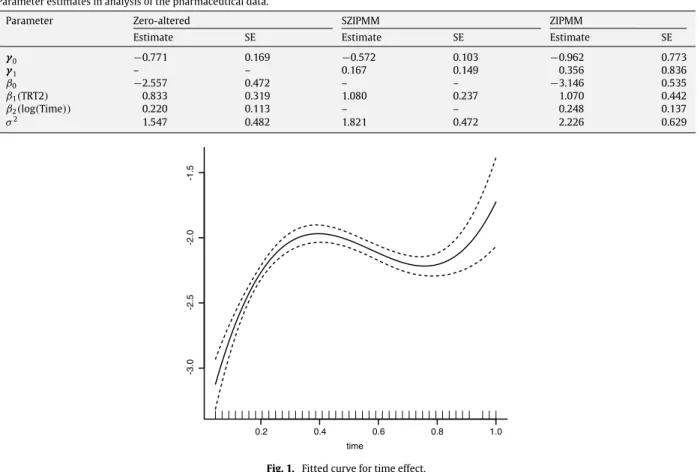
γ0 −0.771 0.169 −0.572 0.103 −0.962 0.773 γ1 – – 0.167 0.149 0.356 0.836 β0 −2.557 0.472 – – −3.146 0.535 β1(TRT2) 0.833 0.319 1.080 0.237 1.070 0.442 β2(log(Time)) 0.220 0.113 – – 0.248 0.137 σ2 1.547 0.482 1.821 0.472 2.226 0.629 0.2 0.4 0.6 0.8 1.0 -3.0 -2.5 -2.0 -1.5 time
Fig. 1. Fitted curve for time effect.
respectively, wherebi
∼
N(
0, σ
2)
. To approximatef(
·
)
, we adopt a three-order penalized splines using the truncated power basis. The smoothing parameterλ
is chosen to beλ
=
4.
281×
10−4.Compared with the results obtained by Min and Agresti [16], results from the ZIP models give the totally different information that the treatment has no effect on which state subjects come from. It indicates that each subject has a fixed probability not to suffer the side effect. One reason for this result is that the occurrence of the side effect is people’s attributes, independent of other external factors. However, when one belongs to the Poisson state, treatment B significantly increased the mean number of episodes of the side effect, which gives the evidence to Min and Agresti’s [16] conclusion that treatment B seems to increase the probability of the side effect. Because from the definition of
φij
, a higher frequency of the episodes means side effects are more likely to occur.When assuming a linear relationship between Time and the link function in zero-altered random effect model and ZIP mixed model, thep-values of the estimated parameter
β
2are 0.0515 and 0.0703 respectively. It is hard to determine whethertime-between-visit has a significant effect on the number of episodes. However, fromFig. 1, the curve estimated by proposed semiparametric model provides some extra information about the Time effect. It gives the evidence of the cutoff values if we want to partition Time into three periods. It is easy to see that from 0 to 0.3, i.e. about 12–13 days after patients take the medicine, the mean number of episodes of the side effect increases, but the time effect will be stable until 0.9, i.e. 40 days, and after that it increases again. If we only analyze the subjects recorded in first 2 weeks under a fully parametric framework, the number of episodes of the side effect significantly increases with Time in the Poisson state at 0.05 level. This increasing trend is also detected by the proposed semiparametric model. Asf
(
time)
retains a high level after two weeks, it is crucial to suppress this increasing trend to avoid the long-term effect. If this is the case, measures should be taken to pull downf(
time)
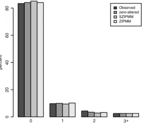
to a much lower level in the first two weeks.To evaluate the prediction performance of the proposed semiparametric model, we plot the probability distribution predicted by the above models and the frequency of the observations for comparison. FromFig. 2, the proposed model has similar performance with the other models in prediction, which suitably describe the number of episodes of the side effect.
5. Simulation study
A simulation study is carried out to study the performance of the proposed estimators. In our simulation, a total of 500 data sets is generated from the considered model with different sample size. We adopt the three-order truncated penalized
Observed zero-altered SZIPMM ZIPMM percent 0 02 0 4 0 6 0 8 0 1 2 3+
Fig. 2. Empirical and predicted frequency distribution of the pharmaceutical data.
Table 3
Simulation results with 500 replications.
ˆ γ0 γˆ1 βˆ σˆ2 Bias 50×4 0.0382 −0.0256 −0.0019 −0.0306 100×4 −0.0094 0.0136 −0.0018 0.0209 150×4 0.0025 −0.0007 −0.0011 0.0151 MCse 50×4 0.3959 0.2335 0.1797 0.3050 100×4 0.2755 0.1634 0.1146 0.2160 150×4 0.2138 0.1234 0.0890 0.1691 AEse 50×4 0.3062 0.1745 0.1496 0.3106 (0.0353) (0.0187) (0.0630) (0.1470) 100×4 0.2159 0.1222 0.1069 0.2190 (0.0176) (0.0088) (0.0324) (0.0680) 150×4 0.1749 0.0992 0.0882 0.1786 (0.0110) (0.0059) (0.0240) (0.0440)
splines and choose the knots as mentioned above. For the smoothing parameter
λ
, we select it over a grid of value ofλ
and use the 20-point grid where the values of log10(λ)
are equally spaced between−
6 and 4 in the simulation models according to our experience in the simulation.We consider the following model:
logit
(
pij)=
γ
0+
γ
1Gij, i=
1, . . . ,
K,
j=
1, . . . ,
Ti log(µij)
=
β
Bij+
sin(
2π
tij)+
bi,
bi ∼N(
0, σ
2),
whereTi
=
4,
γ
0=
1,
γ
1= −
0.
5, β
=
0.
5, σ
2=
1, andGijandBijare drawn independently from uniform distribution on(
0,
3)
and(
0,
2)
respectively, whereastijare drawn from uniform distribution on(
0,
1)
. In order to illustrate the asymptotic properties, we carry out three simulations withK=
50, 100 and 150. Theoreticallyλ
should be chosen for each replicated data set by the GCV method. In practice, for time-saving, we usually conduct several experiments to see whetherλ
varies widely. If not,λ
will be fixed for all the data sets in each simulation. With differentKin our study, the smoothing parameterλ
is chosen to be 4.
429×
10−6, 2.
506×
10−6and 10−6respectively. The bias of the mean of the estimates (Bias), empirical standard deviation (MCse) and the mean of the estimated standard deviation (AEse) are recorded and summarized inTable 3.AEses are calculated according to the sandwich formula provided inTheorem 2by replace the true values with their estimates. They are the consistent estimates of the diagonal elements ofVψ0. The values in the parentheses are the standard error ofAEse.
It is obvious that the estimator of the parametric part works very well and the means of the estimates are very close to their respective true values, even when the number of subjects is not very large. TheAEseof the
σ
ˆ
2is reasonably close totheMCsein the three simulations. TheAEseof
γ
is about 20% smaller than theMCsewithK=
50, 100 and 150. However, the MCseandAEseofβ
ˆ
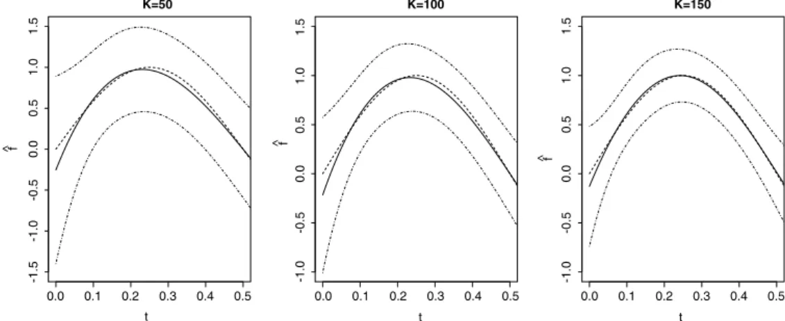
become closer with the increase ofK.Fig. 3shows the estimated curve of the nonparametric function.0.0 0.1 0.2 0.3 0.4 0.5 -1.5 -1.0 -0.5 0.0 0.5 1.0 1.5 K=50 t f^ 0.0 0.1 0.2 0.3 0.4 0.5 -1.0 -0.5 0.0 0.5 1.0 1.5 K=100 t f ^ 0.0 0.1 0.2 0.3 0.4 0.5 -1.0 -0.5 0.0 0.5 1.0 1.5 K=150 t f^
Fig. 3. Plot of the estimated curve forK =50,K =100 andK =150. (The solid line is the estimator and the dashed one is the true curve. The 95% pointwise confidence bands are plotted in dotted lines.)
It is obvious that the estimated one is able to capture the shape offreasonably well. Especially forK
=
150, except at the boundary values, it shows that there is little bias between the true functionfand the estimated one.For further comparison over the three models discussed in the empirical example, we carry out several additional simulations in different setups to show their prediction performances. For lack of space, the model used in the simulation and the detailed results are not shown here. Only the conclusions and discussion from the simulation are provided. Specifically, we focus on the probability of the response to be zero,
φij
=
Pr(
Yij=
0)
, and the mean parameter of the Poisson distribution,µij
. The MSE ofφij
ˆ
andµij
ˆ
are used as the standards of the evaluation. The first simulation assumes a zero-altered random effect model setup, for which both the zero-altered random effect model and the ZIPMM are fitted. The relative efficiency ofφij
ˆ
andµij
ˆ
are 0.
6674 and 0.
8716, respectively. However, in the second simulation of the ZIPMM setup, the two values are 0.
4106 and 0.
9137. The difference between the relative efficiency ofµij
ˆ
under two setups is negligible, whereas the efficiency loss of the zero-altered random effect model under ZIPMM setup is much higher. It indicates in the prediction the probability for the response to be zero, ZIPMM is more stable than the zero-altered random effect model. In the third and fourth simulation, we compare ZIPMM and SZIPMM under different setups. The relative efficiency ofφij
ˆ
andµij
ˆ
are 0.9743 and 0.9477, respectively, when the working model is ZIPMM. In comparison, the two values are 0.7364 and 0.5499 if we assume the SZIPMM in the simulation. It is obvious that our semiparametric method has a much lower efficiency loss than the parametric model. On the basis of above discussion, the proposed model, SZIPMM, has the most stable performance in the prediction ofφij
ˆ
andµij
ˆ
, even if the model is misspecified.In addition, the zero-altered random effect model has the same coefficients of the explanatory variables in both parts, which may lead to some problems in the inference of the covariates. Compared with ZIP regression, another defect of the zero-altered random effect model is the incapability of discriminating which zeros come from the zero state and which are generated by Poisson distribution. In manufacturing process or clinical trials, however, it is more meaningful to explore the environment of the zero state. Because it can help avoid the defects in the course of production or find a safer and more effective treatment. Furthermore, the proposed model in this article is a more robust method compared with the parametric one when some continuous covariate exists. Given these reasons, SZIPMM is a reliable choice in the analysis of longitudinal zero-inflated count data.
6. Discussion
In this article, we consider the longitudinal zero-inflated count data in a semiparametric set up. The proposed semiparametric ZIP mixed model specified in Eqs.(3)and(4)combines the ZIP mixed model and a fully nonparametric function, which is quite useful when the nonlinear effect of some covariates on the link function of the mean of the response variable and the within-subject correlation both exist. A GCV criterion is used to select the smoothing parameter to achieve a good fitting of the nonparametric function. The Monte Carlo expectation–maximization technique is used to reduce the computational burdens of the numerical methods when the dimension of the random effects grows higher.
The performance of the estimators has been shown to be satisfactory, especially when sample size is relatively large. The estimator for the nonparametric functionfis sensitive enough to capture the true shape or pattern off. Generally, the proposed model can be extended to incorporate another unknown smooth function, sayg
(
t)
, and random interceptuito the logistic part so thatlogit
(
pij)=
GTijγ
+
g(
t)
+
ui.The proposed algorithm and theorems developed in this article are still valid with slight modifications. However, the computation will be a little more time-consuming as the dimension of the random effects is higher.
Robust estimation for the generalized partial linear mixed model has attracted more and more attention recently. Xie et al. [25] discussed the example in this article based on an influence diagnostic method and detected the strong influential observation and subject. Hall and Shen [9] proposed robust estimation for zero-inflated Poisson regression. The robustified estimation of our model deserves further study.
Acknowledgments
The authors would like to thank the Editor and the referee for their constructive comments and helpful suggestions that largely improve the presentation of the paper. The research is supported by the Natural Science Foundation of China Grant 10931002, 1091120386.
Appendix
To establish the rootn consistency and asymptotic normality for the proposed estimators, we need the following regularity conditions. Similar conditions are also given in Qin and Zhu [17].
(A) The parametric space Ψ is compact. For any
ψ
∈
Ψ, with probability one, N1GN(
ψ
)
converges uniformly to a nonstochastic functionG(
ψ
)
, which has a unique zero atψ
0∈
Ψ.(B) supi≥1E
|
fz∗ i,bi|yidzidbi|
(2+δ)<
∞
and supi≥1E|
E ∗ zi,bi|yi||
(
zi,bi)| |
2|
(2+δ)<
∞
, where
δ
is some positive constant. (C) (a) There is a neighborhoodC(
ψ
0)
ofψ
0on which with probability one allGN(ψ
)
are continuously differentiable and for∀
ψ
∈
C(
ψ
0)
, the JacobiansN1G˙
N(ψ
)
converges uniformly to a nonstochastic matrixΩ= ˙
G(
ψ
0)
which is nonsingular atψ
0, where 1 N˙
GN(
ψ
0)
=
1 N K−
i=1
∂
∂
γ
TGγ,i(ψ
)
∂
∂
θ
TGγ,i(ψ
)
∂
∂σ
2Gγ,i(
ψ
)
∂
∂
γ
TGθ,i(ψ
)
∂
∂
θ
TGθ,i(ψ
)
∂
∂σ
2Gθ,i(ψ
)
∂
∂
γ
TGσ2,i(ψ
)
∂
∂
θ
TGσ,i(ψ
)
∂
∂σ
2Gσ2,i(
ψ
)
ψ=ψ0.
(b) With probability one,N1
∑
K i=1
Gγ,i(ψ)Gγ,i(ψ)T Gγ,i(ψ)Gθ,i(ψ)T Gγ,i(ψ)Gσ2,i(ψ) Gθ,i(ψ)Gγ,i(ψ)T Gθ,i(ψ)Gθ,i(ψ)T Gθ,i(ψ)G σ2,i(ψ) Gσ2,i(ψ)Gγ,i(ψ)T Gσ2,i(ψ)Gθ,i(ψ)T Gσ2,i(ψ)Gσ2,i(ψ)
ψ =ψ0converges to some positive-definite matrixS.
Proof of Theorem 1. In the proof ofTheorem 1, all the convergences refer to that which holds with probability one unless otherwise stated.
Let
{ ˆ
ψ
N}
be a sequence of the proposed estimators. Letψ
0be the limit point of the sequence of{ ˆ
ψ
N}
; thus there exists a subsequence{ ˆ
ψ
N k}
so that it converges toψ
0. WhenNk→ ∞
, we have
1 NGN(ˆ
ψ
Nk;
λ)
−
G(
ψ
0)
≤
1 NGN(ˆ
ψ
Nk;
λ)
−
1 NGN(ˆ
ψ
Nk)
+
1 NGN(
ˆ
ψ
Nk)
−
G(
ˆ
ψ
Nk)
+
G(
ˆ
ψ
Nk)
−
G(
ψ
0)
.
Ifλ
=
o(
1)
, then
1 NGN(ˆ
ψ
Nk;
λ)
−
1 NGN(ˆ
ψ
Nk)
→
0.
By condition (A), it follows that
1 NGN(ˆ
ψ
Nk)
−
G(
ˆ
ψ
Nk)
→
0.
As{ ˆ
ψ
N k}
converges toψ
0, we have G(
ψ
ˆ
Nk)
−
G(
ψ
0)
→
0.
Therefore,
1 NGN(ˆ
ψ
Nk;
λ)
−
G(
ψ
0)
→
0.
Sinceψ
ˆ
Nkis the solution ofGN
(
ψ
;
λ)
=
0, then
G(
ψ
0)
=
0, i.e.ψ
0is the zero ofG(
ψ
)
. Furthermore, becauseψ
0is theunique zero ofG
(
ψ
)
, the limit pointψ
0must beψ
0. On the other hand,ψ
0is the limit point of any convergent subsequence. Therefore,ψ
ˆ
N→
ψ
0with probability one.Proof of Theorem 2. By the mean value theorem, we have GN
(
ψ
;
λ)
=
GN(ψ
0;
λ)
+ ˙
GN(ψ
∗;
λ)(
ψ
−
ψ
0),
whereψ
∗=
ψ
0+
τ
ψ
, 0< τ <
1. Replaceψ
ˆ
byψ
,√
N(
ψ
ˆ
−
ψ
0)
=
−
1 N˙
GN(ψ
∗;
λ)
−1
1√
NGN(
ψ
0;
λ)
.
Ifλ
=
o(
1/
√
N)
, √1 NNλ
Rα
=
op(1)
. Asˆ
ψ
is the consistent estimate ofψ
, and by condition (C)(a), whenN→ ∞
, we have1 NG
˙
N(
ψ
∗
;
λ)
→
1NG
˙
N(ψ
0)
→
Ω. From condition (B), it follows that supi≥1E
Gi(
ψ
0)
(2+δ)
<
∞
. Then by condition (A)(b) and central limit theorem,√1NGN
(
ψ
0)
L→
N(
0,
S)
.Theorem 2is obtained. References[1] S.C. Barry, A.H. Welsh, Generalized additive modelling and zero inflated count data, Ecological Modelling 157 (2002) 179–188.
[2] D. Bohning, E. Dietz, P. Schlattmann, L. Mendonca, U. Kirchmer, The zero-inflated Poisson model and the decayed, missing and filled teeth in index in dental epidemiology, Journal of the Royal Statitscal Society, Series A 162 (Part2) (1999) 195–209.
[3] Y.B. Cheung, Zero-inflated models for regression analysis of count data: a study for growth and development, Statistics in Medicine 21 (2002) 1461–1469.
[4] M. Chiogna, C. Gaetan, Semiparametric zero-inflated Poisson models with application to animal abundance studies, Environmetrics 18 (2007) 303–314.
[5] A.C. Cohen, Estimation in mixtures of discrete distributions, in: Proceedings of the International Symposium on Discrete Distributions, Montreal, 1963, pp. 73-378.
[6] M.J. Dobbie, A.H. Welsh, Modelling correlated zero-inflated count data, Australian & New Zealand Journal of Statistics 43 (2001) 431–444. [7] D.B. Hall, Zero-inflated Poisson and binomial regression with random effects: a case study, Biometrics 56 (2000) 1030–1039.
[8] D.B. Hall, Z.G. Zhang, Marginal models for zero inflated clustered data, Statistical Modelling 4 (2004) 161–180.
[9] D.B. Hall, J. Shen, Robust estimation for zero-inflated Poisson regression, Scandinavian Journal of Statistics 36 (2009) Early view. [10] N.L. Johnsen, S Kotz, Distributions in Statistics: Discrete Distribution, Houghton Mifflin, Boston, 1969.
[11] D. Lambert, Zero-inflated Poisson regression, with an application to defects in manufacturing, Technometrics 34 (1992) 1–14. [12] K.F. Lam, H.Q. Xue, Y.B. Cheung, Semiparametric analysis of zero-inflated count data, Biometrics 62 (2006) 996–1003. [13] K-Y. Liang, S.L. Zeger, Longitudinal data analysis using generalized linear models, Biometrika 73 (1986) 13–22.
[14] X. Lin, R.J. Carroll, Semiparametric regression for clustered data using generalized estimating equations, Journal of the American Statistical Association 96 (2001) 1045–1056.
[15] C.E. McCulloch, Maximum likelihood algorithm for generalized linear mixed models, Journal of American Statistical Assosiation 92 (1997) 162–170. [16] Y.Y. Min, A. Agresti, Random effect models for repeated measures of zero-inflated count data, Statistical Modelling 5 (2005) 1–19.
[17] G.Y. Qin, Z.Y. Zhu, Robustified maximum likelihood estimation in gerneralized partial linear mixed model for longitudinal data, Biometrics 65 (2009) 52–59.
[18] A. Qu, R.Z. Li, Quadratic Inference functions for varying-coefficient models with longitudinal data, Biometrics 62 (2006) 379–391. [19] C.P. Robert, G. Casella, Monte Carlo Statistical Methods, Springer-Verlag, New York, 1999.
[20] D. Ruppert, M.P. Wand, R.J. Carroll, Semiparametric Regression, Edinburgh, Cambridge, 2003.
[21] V. Shankar, J. Milton, F. Mannering, Modeling accident frequencies as zero-altered probability processes: an empirical inquiry, Accident Analysis and Prevention 29 (1997) 829–837.
[22] K. Wang, K.K.W. Yau, A.H. Lee, A zero-inflated Poisson mixed model to analyze diagnosis related groups with majority of same-day hospital stays, Computer methods and programs in Biomedicine 68 (2002) 195–203.
[23] A.H. Welsh, R.B. Cunningham, C.F. Donnelly, D.B. Lindenmayer, Modelling the abundance of rare species: statistical models for counts with extra zeros, Ecological Modelling 88 (1996) 297–308.
[24] H.Y. Xie, G. McHugo, A. Sengupta, R. Clark, R. Drake, A method for analyzing longitudinal outcomes with many zeros, Mental Health Services Research 6 (2004) 239–246.
[25] F.C. Xie, B.C. Wei, J.G. Lin, Assessing influence for pharmaceutical data in zero-inflated generalized Poisson mixed models, Statitics in Medicine 27 (2008) 3656–3673.
[26] Y. Yu, D. Ruppert, Penalized spline estimation for partially linear single index models, Journal of the American Statistical Association 97 (2002) 1042–1054.