UCLA
UCLA Electronic Theses and Dissertations
TitleExact Diffusion Learning over Networks
Permalink https://escholarship.org/uc/item/7z3677dm Author Yuan, Kun Publication Date 2019 Peer reviewed|Thesis/dissertation
UNIVERSITY OF CALIFORNIA Los Angeles
Exact Diffusion Learning over Networks
A dissertation submitted in partial satisfaction of the requirements for the degree
Doctor of Philosophy in Electrical and Computer Engineering
by
Kun Yuan
c
Copyright by Kun Yuan
ABSTRACT OF THE DISSERTATION Exact Diffusion Learning over Networks
by Kun Yuan
Doctor of Philosophy in Electrical and Computer Engineering University of California, Los Angeles, 2019
Professor Ali H. Sayed, Chair
In this dissertation, we study optimization, adaptation, and learning problems over connected networks. In these problems, each agent k collects and learns from its own local data and is able to communicate with its local neighbors. While each single node in the network may not be capable of sophisticated behavior on its own, the agents collaborate to solve large-scale and challenging learning problems.
Different approaches have been proposed in the literature to boost the learning capabili-ties of networked agents. Among these approaches, the class of diffusion strategies has been shown to be particularly well-suited due to their enhanced stability range over other methods and improved performance in adaptive scenarios. However, diffusion implementations suffer from a small inherent bias in the iterates. When a constant step-size is employed to solve deterministic optimization problems, the iterates generated by the diffusion strategy will converge to a small neighborhood around the desired global solution but not to the exact solution itself. This bias is not due to any gradient noise arising from stochastic approxima-tion; it is instead due to the update structure in diffusion implementations. The existence of the bias leads to three questions: (1) What is the origin of this inherent bias? (2) Can it be eliminated? (3) Does the correction of the bias bring benefits to distributed optimization, distributed adaptation, or distributed learning?
This dissertation provides affirmative solutions to these questions. Specifically, we design a newexact diffusionapproach that eliminates the inherent bias in diffusion. Exact diffusion
has almost the same structure as diffusion, with the addition of a “correction” step between the adaptation and combination steps. Next, this dissertation studies the performance of exact diffusion for the scenarios of distributed optimization, distributed adaptation, and dis-tributed learning, respectively. For disdis-tributed optimization, exact diffusion is proven to con-verge exponentially fast to theexactglobal solution under proper conditions. For distributed adaptation, exact diffusion is proven to have better steady-state mean-square-error than dif-fusion, and this superiority is analytically shown to be more evident for sparsely-connected networks such as line, cycle, grid, and other topologies. In distributed learning, exact dif-fusion can be integrated with the amortized variance-reduced gradient method (AVRG) so that it converges exponentially fast to the exact global solution while employing stochastic gradients per iteration. This dissertation also compares exact diffusion with other state-of-the-art methods in literature. Intensive numerical simulations are provided to illustrate the theoretical results derived in the dissertation.
The dissertation of Kun Yuan is approved.
Wotao Yin Lieven Vandenberghe
Lara Dolecek
Ali H. Sayed, Committee Chair
University of California, Los Angeles 2019
TABLE OF CONTENTS
1 Introduction . . . 1
1.1 Problem Formulation . . . 2
1.1.1 Distributed Optimization . . . 3
1.1.2 Distributed Adaptation and Online Learning . . . 4
1.1.3 Distributed Empirical Machine Learning . . . 5
1.2 Diffusion Learning . . . 7
1.2.1 Diffusion for Distributed Optimization . . . 7
1.2.2 Diffusion for Distributed Adaptation and Online Learning . . . 10
1.2.3 Diffusion for Distributed Empirical Machine Learning . . . 11
1.3 Objectives and Organization . . . 13
1.4 Notation . . . 16
2 Exact Diffusion for Distributed Optimization: Algorithm Development 17 2.1 Context and Background . . . 17
2.1.1 Related Work . . . 17
2.1.2 Motivation and Contributions . . . 20
2.2 Diffusion and Combination Policies . . . 23
2.2.1 Standard Diffusion Strategy . . . 23
2.2.2 Combination Policy . . . 25
2.2.3 Values of Balanced Left-stochastic Policies . . . 31
2.2.4 Necessity of Locally Balanced Condition . . . 33
2.2.5 Useful Properties . . . 34
2.3.1 Constrained Problem Formulation . . . 38
2.3.2 Penalized Formulation . . . 39
2.4 Development of Exact Diffusion . . . 41
2.5 Significance of Balanced Policies . . . 44
2.6 Numerical Experiments . . . 49
2.6.1 Distributed Least-squares . . . 49
2.6.2 Distributed Logistic Regression . . . 50
2.6.3 Benefits of Balanced Left-stochastic Policies . . . 51
2.6.4 Exact Diffusion for General Left-Stochastic A . . . 53
2.7 Concluding Remarks . . . 55
2.A Formulation of Primal Methods . . . 56
2.A.1 Consensus Strategy . . . 57
2.A.2 Diffusion Strategy . . . 57
2.A.3 Other Primal Methods . . . 58
2.B Formulation of Primal-Dual Methods . . . 58
2.B.1 EXTRA Method . . . 58
2.B.2 Exact Diffusion Method . . . 59
2.B.3 Tracking Method . . . 60
2.B.4 Distributed ADMM . . . 61
2.C Formulation of Dual Methods . . . 63
2.D Proof of (2.116) . . . 65
3 Exact Diffusion for Distributed Optimization: Convergence Analysis . . 69
3.1 Convergence of Exact Diffusion . . . 69
3.1.2 Error Recursion . . . 72
3.1.3 Proof of Convergence . . . 74
3.2 Stability Comparison with EXTRA . . . 80
3.2.1 Stability Range of EXTRA . . . 80
3.2.2 Comparison of Stability Ranges . . . 83
3.2.3 An Analytical Example . . . 85
3.3 Numerical Experiments . . . 89
3.3.1 Distributed Least-squares . . . 89
3.3.2 Distributed Logistic Regression . . . 92
3.A Proof of Lemma 3.3 . . . 93
3.B Proof of Theorem 3.1 . . . 97
3.C Proof of Theorem 3.2 . . . 104
3.D Error Recursion for EXTRA Consensus . . . 111
3.E Error Recursion in Transformed Domain . . . 112
3.F Proof of Theorem 3.3 . . . 114
3.G Proof of Lemma 3.5 . . . 117
3.H Proof of Lemma 3.6 . . . 119
4 Exact Diffusion For Distributed Adaptation and Online Learning . . . . 121
4.1 Introduction . . . 121
4.1.1 Main Results . . . 123
4.1.2 Related work . . . 126
4.2 Exact Diffusion Strategy . . . 127
4.3 Error Dynamics of Exact Diffusion . . . 128
4.3.2 Transformed Error Dynamics . . . 131
4.4 Mean-square Convergence . . . 132
4.4.1 Well-connected Network . . . 135
4.4.2 Sparsely-connected Network . . . 136
4.5 Mean-square Deviation Expression . . . 138
4.5.1 Approximate Error Dynamics . . . 138
4.5.2 Deriving the MSD expression . . . 140
4.6 Numerical Simulation . . . 143
4.6.1 Mean-square-error Network . . . 143
4.6.2 Distributed Logistic Regression . . . 147
4.6.3 Comparison with Gradient Tracking Methods . . . 149
4.7 Conclusion . . . 150
4.A Proof of Theorem 4.1 . . . 152
4.B Proof of Lemma 4.5 . . . 159
4.C Proof of Theorem 4.2 . . . 164
5 Exact Diffusion for Distributed Empirical Learning . . . 169
5.1 Context and Background . . . 169
5.1.1 Problem Formulation . . . 170
5.1.2 Related Work . . . 171
5.1.3 Contribution . . . 172
5.2 Two Key Components . . . 173
5.2.1 Exact Diffusion Algorithm . . . 174
5.2.2 Amortized Variance-Reduced Gradient (AVRG) Algorithm . . . 175
5.4 Diffusion–AVRG Algorithm for Unbalanced Data Distributions . . . 178
5.4.1 Comparison with Decentralized SVRG . . . 180
5.5 Diffusion-AVRG with Mini-batch Strategy . . . 180
5.6 Simulation Results . . . 182
5.A Proof of Theorem 5.1 . . . 187
5.A.1 Extended Network Recursion . . . 188
5.A.2 Optimality Condition . . . 189
5.A.3 Error Dynamics . . . 190
5.A.4 Useful Inequalities . . . 193
5.A.5 Linear Convergence . . . 195
5.B Proof of recursion (5.56) . . . 196
5.C Proof of recursion (5.61) . . . 197
5.D Proof of Lemma 5.1 . . . 199
5.E Proof of Lemma 5.2 . . . 201
5.F Proof of Lemma 5.3 . . . 205
5.G Proof of Lemma 5.4 . . . 207
5.H Proof of Lemma 5.5 . . . 212
5.I Upper Bound on (1−a1µν)Ns . . . 217
5.J Proof of Lemma 5.6 . . . 217
5.K Proof of Theorem 5.7 . . . 223
6 Conclusion and Future Work . . . 232
LIST OF FIGURES
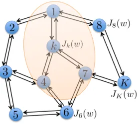
1.1 An illustration of the network. The network is connected, and each agent holds a local cost function Jk(w). The arrow refers to communication. For example, agent k can
send/receive information to/from its immediate neighbors{1,4,7}. The yellow shadow indicates the neighboring set of agent k. . . 4
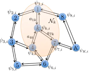
1.2 An illustration of the combination step (1.6) in diffusion method. SinceNk={1,4,7, k},
it holds that wk,i=P`∈Nka`kψ`,i=a1kψ1,i+a4kψ4,i+a7kψ7,i+akkψk,i. . . 9
2.1 Illustration of the local balance condition (2.13). . . 27 2.2 Illustration of the relations among the classes of symmetric doubly-stochastic, balanced
left-stochastic, and left-stochastic combination matrices. . . 31 2.3 Network topology used in the simulations. . . 49 2.4 Convergence comparison between standard diffusion and exact diffusion for the distributed
least-squares (2.121). . . 50 2.5 Convergence comparison between standard diffusion and exact diffusion for distributed logistic
regression (2.122). . . 51 2.6 A highly unbalanced network topology. . . 53 2.7 Convergence comparison between exact diffusion and EXTRA for highly unbalanced network.
Exact diffusion is with the averaging rule while EXTRA is with the doubly stochastic rule.. . 54 2.8 Convergence comparison between exact diffusion and EXTRA for the scenario in which local
Lipschitz constants differ drastically. Exact diffusion is with the Hastings rule (2.40) while EXTRA is with the doubly stochastic rule. . . 54 2.9 Exact diffusion under the setting of Example 1 in Section 2.5. Top: ρ >1 no matter what value
µis. Bottom: Convergence comparison between diffusion and exact diffusion whenµ= 0.01. 55 2.10 Exact diffusion under the setting of Example 2 in Section 2.5. Top: ρ < 1 when µ < 0.2.
Bottom: Convergence comparison between standard diffusion and exact diffusion when µ = 0.001. . . 55
2.11 The Jury table for the 7-th order system. . . 68
3.1 A two-agent network using combination weights{a,1−a} . . . 86
3.2 Convergence comparison between exact diffusion, EXTRA, DIGing, and Aug-DGM for dis-tributed least-squares problem (3.119). In the top plot, the step-sizes for Exact diffusion, EXTRA, DIGing and Aug-DGM are 0.013, 0.007, 0.0028 and 0.003. In the bottom plot, all step-sizes are set as 0.04. . . 91
3.3 Convergence comparison between exact diffusion, EXTRA, DIGing, and Aug-DGM for dis-tributed least-squares problem (3.119) with non-symmetric combination policy. . . 92
3.4 Convergence comparison between exact diffusion, EXTRA, DIGing, and Aug-DGM for problem (3.120). In the top plot, the step-sizes for Exact Diffusion, EXTRA, DIGing and AUG-DGM are 0.041, 0.028, 0.014 and 0.033. In the bottom plot, all step-sizes are set as 0.04. . . 94
4.1 Performance of Exact Diffusion and Diffusion under different scenarios . . . 125
4.2 Illustration of the grid topology and cyclic topology. . . 137
4.3 Diffusion v.s. exact diffusion over grid networks for problem (4.73). . . 141
4.4 The superiority of exact diffusion is more evident as the grid network becomes larger when solving problem (4.73). . . 142
4.5 Diffusion v.s. exact diffusion over a fully connected network for problem (4.73). 145 4.6 Diffusion v.s. exact diffusion over cyclic networks for problem 4.75. . . 146
4.7 The superiority of exact diffusion gets more evident as the cyclic networks gets larger when solving problem 4.75. . . 147
4.8 Diffusion v.s. exact diffusion over a fully connected network for problem (4.75). 148 4.9 Comparison between diffusion [1], exact diffusion (proposed), and gradient track-ing [2, 3] over cyclic networks for problem (4.73). . . 149
4.10 Comparison between diffusion [1], exact diffusion (proposed), and gradient track-ing [2, 3] over a fully connected network when solvtrack-ing problem (4.73). . . 151
5.1 Illustration of the operation of diffusion-AVRG for a two-node network.. . . 179 5.2 Illustration of what would go wrong if one attempts a diffusion-SVRG implementation
for a two-node network, and why diffusion-AVRG is the recommended implementation. 182 5.3 Comparison between diffusion-AVRG and DSA over various datasets. Top: data are
evenly distributed over the nodes; Bottom: data are unevenly distributed over the nodes. The average sample size is Nave =
PK
k=1Nk/K. . . 183
5.4 A random connected network with 20 nodes. . . 184 5.5 Diffusion-AVRG is more stable than DSA. . . 184 5.6 Performance of diffusion-AVRG with different batch sizes on MNIST dataset. Each
agent holds Ns = 1200 data. . . 186
5.7 Performance of diffusion-AVRG with different batch sizes on RCV1 dataset. Each agent holds Ns = 480 data. . . 187
LIST OF TABLES
ACKNOWLEDGMENTS
First and foremost, I would like to express my sincere gratitude to my advisor Professor Ali H. Sayed. Working at the Adaptive Systems Laboratory at UCLA has been one of the most challenging and rewarding experiences in my life. Professor Sayed’s high standards in research, careful review of my papers, and numerous valuable suggestions greatly enhanced the quality of my work. Moreover, some of his advice such as “focus on good work” and “Do not simply follow the other people’s ideas, figure it out your own way” have become my motto at work.
I am also grateful to Prof. Wotao Yin for his generous help and insightful discussions during my five years stay at UCLA. It is always fun and pleasant to work with him. I would also like to thank Prof. Lara Dolecek and Prof. Lieven Vandenberghe for serving on my doctoral committee, and for their valuable advice and feedback during the thesis defense.
My research would not have been easy without having great and supportive collaborators: Bicheng Ying, Sulaiman A. Alghunaim, Stefan Vlaski, Tianyu Wu, Lucas Cassano, Ernest K. Ryu, Jiageng Liu, Xianghui Mao, Prof. Qing Ling and Prof. Yuantao Gu. I learned a lot from all of them. I also appreciate the time I spent with many good friends at UCLA, EPFL and Microsoft Research. They are Zhimin Peng, Lanchao Liu, Jialin Liu, Yanli Liu, Hanqin Cai, Fei Feng, Yuejiao Sun, Robert Hannah, Hawraa Salami, Chung-Kai Yu, Chengcheng Wang, Jianshu Chen, Edward Nguyen, Eric Tan, Gabrielle Robertson, Roula Nassif, Xiujun Li, Zhirui Zhang, Shuohang Wang and Jinchao Li.
Furthermore, I want to thank my family for their unconditional support. In particular, I wish to express my deepest love to my wife Yang and my son Max. It is them who motivate me to keep working hard and moving forward.
This dissertation is based on work partially supported by the National Science Foundation under grants CCF-1524250 and ECCS-1407712. Any opinions, findings, and conclusions or recommendations expressed in this material are those of the author and do not necessarily reflect the views of the National Science Foundation.
VITA
2007–2011 B.S., Dept. Electrical and Engineering, Xidian University, Xi’an, China.
2011–2014 M.S., Dept. Electrical and Engineering, University of Science and Tech-nology of China (USTC), Hefei, China.
2014–2019 Research Assistant, Dept. Electrical and Computer Engineering, Univer-sity of California, Los Angeles (UCLA), CA, USA
2018 Intern, Microsoft Research, Redmond, WA, USA
2018 Visiting Student, Ecole Polytechnique Federale de Lausanne (EPFL), Switzerland
PUBLICATIONS
S. A. Alghunaim, K. Yuan, A. H. Sayed, “A linearly convergent proximal gradient algorithm for decentralized optimization”, Proc. Neural Information Processing Systems (NeurIPS), 2019.
B. Ying, K. Yuan, A. H. Sayed, “Dynamic average diffusion with randomized coordinate updates”, to appear in IEEE Trans. Signal and Information Processing over Networks, 2019.
S. A. Alghunaim, K. Yuan, A. H. Sayed, “A proximal diffusion strategy for multi-agent optimization with sparse affine constraints”, to appear in IEEE Trans. Automatic Control,
2019.
K. Yuan, B. Ying, X. Zhao, and A. H. Sayed, “Exact diffusion for distributed optimization and learning – Part I: Algorithm development,” IEEE Trans. Signal Processing, vol. 67, no. 3, pp. 708-723, Feb. 2019.
K. Yuan, B. Ying, X. Zhao, and A. H. Sayed, “Exact diffusion for distributed optimization and learning – Part II: Convergence analysis,” IEEE Trans. Signal Processing, vol. 67, no. 3, pp. 724-739, Feb. 2019.
B. Ying, K. Yuan, and A. H. Sayed, “Supervised learning under distributed features,” IEEE Trans. Signal Processing, vol. 67, no. 4, pp. 977-992, Feb. 2019.
B. Ying, K. Yuan, S. Vlaski, and A. H. Sayed, “Stochastic learning under random reshuffling with constant step-sizes,” IEEE Trans. Signal Processing, vol. 67, no. 2, pp. 474-489, Jan. 2019.
K. Yuan, B. Ying, J. Liu, A. H. Sayed, “Variance-reduced stochastic learning by networked agents under random reshuffling”, IEEE Trans. Signal Processing, vol. 67, no. 2, pp. 351-366, Jan. 2019.
T. Wu, K. Yuan, Q. Ling, W. Yin, and A. H. Sayed, “Decentralized consensus optimiza-tion with asynchrony and delays,” IEEE Trans. Signal and Information Processing over Networks, vol. 4, no. 2, pp. 293-307, Jun. 2018.
K. Yuan, B. Ying, and A. H. Sayed, “On the influence of momentum acceleration on online learning,” Journal of Machine Learning Research, vol. 17, no. 192, pp. 1-66, 2016.
CHAPTER 1
Introduction
In this dissertation, we study optimization, adaptation, and learning problems over connected networks. In these problems, each agent k collects and learns from its own local data and is able to communicate with its local neighbors. While each single node in the network may not be capable of sophisticated behavior on its own, it is the interaction among the constituents that leads to a powerful system that is able to solve large-scale and more challenging problems [1, 4].
Different approaches have been proposed in the literature to boost the learning capabili-ties of networked agents. Among them, the class of diffusion strategies [5–13] has been shown to be particularly well-suited due to their improved stability range over other methods and enhanced performance in adaptive scenarios. In particular, references [1, 4] study diffusion closely and explain how the diffusion strategy (a) performs distributed optimization over networks; (b) performs distributed adaptation over networks; (c) and performs distributed learning over networks. By quantifying the behavior of the algorithm, it is shown that diffusion will improve the averaged performance across the network.
It is known that diffusion implementations suffer from a small inherent bias [14]. When employing a constant step-size to solve a deterministic optimization problem, the iterates generated by the diffusion strategy will converge to a small neighborhood around the desired global solution but not to the exact solution itself. This inherent bias is not due to any gradient noise arising from stochastic approximation; it is instead due to the update structure in diffusion implementations [15, 16]. The existence of the bias in diffusion leads to three questions:
2. Can we eliminate the bias?
3. Does the correction of the bias bring benefits to distributed optimization, distributed adaptation, or distributed learning?
In the coming chapters, we will present results that allow us to answer the above useful questions in the affirmative. To be specific, we will propose a new method exact diffusion that eliminates the inherent bias in Chapter 2. Furthermore, we will show whether, when and why exact diffusion can outperform diffusion for optimization, adaptation, and learning scenarios in Chapters 2–5. We will also compare the performance of exact diffusion to other state-of-the-art algorithms in the literature.
In this chapter, we will briefly discuss the problem formulation in distributed optimiza-tion, distributed adaptation and online learning, and distributed empirical machine learning, respectively. Next we will review the diffusion strategy in detail and present its various forms when solving problems in each of the above scenarios.
1.1
Problem Formulation
Consider a connected and undirected networkG = (V,E) where V is the set of all networked nodes with |V| = K while E is the set of all edges. The optimization problem defined over this network is to let each agent operate cooperatively to solve a problem of a form
min w∈RM Jo(w) = 1 K K X k=1 Jk(w), (1.1)
whereM is the dimension of the variable,Jk(w) :RM →Ris a convex and differentiable cost
function at agent k, and Jo(w) :
RM →Ris the global cost function. We letwo denote the
global minimizer of problem (1.1). While each agent can only access the local cost function
Jk(w), the target of the network is to let all agents collaborate to seek the global solutionwo.
Different from the centralized network topology, e.g., the parameter server [17, 18], where there is a central node connected to all computing agents that is responsible for aggregating and scattering local variables, the network topology considered in the dissertation can take
arbitrary form such as line, cycle, grid, or random geometric graphs. There exists no central node in the considered network topology, and each agent will exchange information with their directly-connected neighbors rather than with a central agent. An illustration of such multi-agent network is shown in Fig. 1.1.
There are many advantages to distributed processing. First, the communication in dis-tributed algorithms is more balanced. With each agent exchanging information with its neighbors, the communication load is evenly distributed over the edges. This is in contrast to centralized algorithms that usually induce great traffic jam on the central node. When the bandwidth around the central server is limited, the performance of centralized algorithms can be significantly degraded. Second, distributed algorithms are more robust to failure of agents. Note that each agent in a distributed strategy plays the same role by conducting the same operations – they update local variables and exchange information with neighbors. When one agent is down, the other agents can still work normally provided the network re-mains connected. In comparison, centralized strategies are more sensitive to the collapse of the central node which coordinates the computation and communication of all agents. Third, in real-time applications where agents collect data continuously, the repeated exchange of information back and forth between the agents and the fusion center can be costly especially when these exchanges occur over wireless links or require nontrivial routing resources. Fi-nally, in some sensitive applications, agents may be reluctant to share their data with remote centers for various reasons including privacy and secrecy considerations.
Problem (1.1) is quite general and it covers various important scenarios by choosing different forms forJk(w). We next discuss these scenarios and their applications.
1.1.1 Distributed Optimization
When each local cost functionJk(w) is known and its gradient∇Jk(w) can be accessed easily,
we regard (1.1) as a distributed optimization problem. This is a deterministic setting and no gradient noise exists to pollute ∇Jk(w). Distributed Optimization is the foundation to
Figure 1.1: An illustration of the network. The network is connected, and each agent holds a local cost function Jk(w). The arrow refers to communication. For example, agent k can send/receive
information to/from its immediate neighbors{1,4,7}. The yellow shadow indicates the neighboring set of agentk.
into the latter scenarios. Distributed optimization finds applications in a wide range of areas in signal processing, control and communication including wireless sensor networks [19–23], event detection [24,25], spectrum sensing of cognitive radios [26,27], vehicle and multi-robot control systems [28, 29], cyber-physical systems and smart grid implementations [30– 33], and many others.
1.1.2 Distributed Adaptation and Online Learning
If Jk(w) is defined as the expectation of some loss function, then problem (1.1) falls into
the scenario of distributed adaptation and online learning. To be concrete, distributed adaptation and online learning consider problems of the form
min w∈RM J(w) = 1 K K X k=1 Jk(w), where Jk(w) =EQ(w;xk). (1.2)
The random variable xk represents the streaming data observed by agent k, and Q(w;xk)
is some loss function such as least-squares or the logistic function. Since the distribution of data xk is generally unknown in advance, we cannot access the cost function Jk(w) and its
realization of dataxk at iterationi. Also, throughout the adaptation setting we assume data
samples xk,i keep streaming in and the underlying distribution may drift with time. Such
drifting distribution may cause a shift in the location of the global minimizer wo, and one
has to design strategies that enable agents to respond in real-time to drifts in data.
Problems of the form (1.2) are prevalent in adaptation and online learning contexts. Typical applications can be found in distributed estimation [1, 4, 14, 34–36], dictionary learn-ing [37–39], clusterlearn-ing [40, 41], multi-task learnlearn-ing [42], distributed feature learnlearn-ing [43], multi-target tracking [44, 45], social learning [46, 47], and multi-agent reinforcement learn-ing [48–51].
1.1.3 Distributed Empirical Machine Learning
Many machine learning problems can be modeled as the empirical risk minimization min w∈RM 1 N N X n=1 Q(w;xn) (1.3)
where xn is the n-th data, N is the size of the dataset, and Q(w;xn) is some loss function
as we discussed in Sec. 1.1.2. When the data size N is very large, it is usually intractable or inefficient to solve problem (1.3) with a single machine. To relieve this difficulty, one solution is to divide theN data samples across multiple machines and solve problem (1.3) in a cooperative manner. To this end, we consider K agents that are connected over the graph
G = (V,E). For each agent k, we assign L =N/K data samples to it, which we denote by
{xk,n}Ln=1. That is, it holds that{xn}Nn=1 ={{x1,n}Ln=1,· · · ,{xK,n}Ln=1}. One can verify that
the empirical risk minimization problem (1.3) is equivalent to min w∈RM 1 K K X k=1 Jk(w) where Jk(w) = 1 L L X n=1 Q(w;xk,n). (1.4)
We regard problem (1.4) as the distributed empirical machine learning problem because it deals with finite, non-streaming, data samples. Since the data samples are fixed, the solution to problem (1.4) is also static.
In large-scale machine learning problems with enormous data to be processed, the number of computing agents K is usually far less than the sample size N. In this case, the size of
the local dataset L can still be very large. Note that each Jk(w) in (1.4) is the average
of L local loss functions, and its gradient ∇Jk(w) = L1 PL
n=1∇Q(w;xk,n) is expensive to
calculate especially for large L. Therefore, one usually employs the gradient over a single data sample∇Q(w;xk,n), or the gradient over a batch of data samples B1
PB
b=1∇Q(w;xk,b),
to approximate the real gradient ∇Jk(w). This constitutes the major difference between
algorithms in distributed optimization and in distributed empirical machine learning. Distributed machine learning over the centralized network, i.e., a network with a central node that is connected to all nodes, is well-studied to speed up training efficiency when large data samples exist. Many useful algorithms exist such as parallel stochastic gradient descent (SGD) methods [52, 53], distributed second-order methods [54–56], parallel dual coordinate methods [57, 58], and distributed alternating direction method of multipliers (ADMM) [59, 60]. However, the information congestion around the central node limits the speedup of these centralized methods, and this motivates great interest in distributed algorithms. For example, references [61, 62] find distributed algorithms, by eliminating the central node, are empirically shown to converge faster than centralized counterparts in deep learning when the network has limited bandwidth or high latency.
Another attractive emerging application for distributed empirical machine learning is fed-erated learning [63, 64]. Fedfed-erated learning is a distributed training approach which enables personal devices, e.g., mobile phones, tablets, and the wearables, located at different geo-graphical positions to collaboratively learn a global machine learning model while keeping all the private data on the device. Current research mainly employs the centralized approaches for federated learning, see [63–66]. However, the convergence time for the federated learning process is significantly slow due to the limited communication bandwidth around the central server and the long communication latency between server and clients. As a result, dis-tributed approaches without central server are introduced for federated learning [67–69] to speed up the convergence with more balanced communication load and short communication ranges.
1.2
Diffusion Learning
Research in distributed optimization dates back several decades (see, e.g., [70] and the ref-erences therein). In recent years, various centralized optimization methods such as (sub-)gradient descent, proximal gradient descent, (quasi-)Newton method, dual averaging, alter-nating direction method of multipliers (ADMM), and many other primal-dual methods have been extended to the distributed setting.
Distributed algorithms that are based on gradient-descent methods are effective and easy to implement. There are at least two prominent variants under this class: the consensus strategy [5–13] and the diffusion strategy [1, 4, 34, 36, 71]. There is a subtle but critical difference in the order in which computations are performed under these two strategies. In the consensus implementation, each agent runs a gradient-descent type iteration, albeit one where the starting point for the recursion and the point at which the gradient is approximated arenotidentical. This construction introduces an asymmetry into the update relation, which has some undesirable instability consequences (described, for example, in Secs. 7.2–7.3, Example 8.4, and also in Theorem 9.3 of [1] and Sec. V.B and Example 20 of [4]). The diffusion strategy, in comparison, employs a symmetric update where the starting point for the iteration and the point at which the gradient is approximated coincide. This property results in a wider stability range for diffusion strategies [1, 4].
In this section we review the diffusion learning algorithm and its recursions in various problem settings. In particular, we will reveal that diffusion, similar to consensus, suffers from an inherent limiting bias which may deteriorate its steady-state performance. This motivates us to study approaches that remove bias.
1.2.1 Diffusion for Distributed Optimization
To proceed, we consider solving problem (1.1) over a connected network of agents. The standard diffusion strategy [1, 4, 34] is listed in Algorithm 1.1 where the first step (1.5) conducts local gradient descent with constant step-sizeµ, and the second step (1.6) conducts weighted averaging for received information with a`k to scale variables flowing from agent `
Algorithm 1.1 Diffusion strategy for distributed optimization at agent k
Setting: Initialize wk,−1 arbitrarily. Repeat for i= 0,1,2,· · ·
ψk,i =wk,i−1−µ∇Jk(wk,i−1), (adaptation) (1.5) wk,i =
X
`∈Nk
a`kψ`,i. (combination) (1.6)
tok. The weights {a`k}K
`=1,k=1 are nonnegative and they satisfy
a`k
≥0 if agents ` and k are connected,
= 0 if agents ` and k are not connected,
a`k =ak`, and X
`∈Nk
a`k = 1 (1.7)
With condition (1.7), it follows that the weight matrix A = [a`k] ∈ RK×K is a symmetric
and doubly-stochastic matrix, i.e.,
A=AT and A1K =1K. (1.8)
Moreover, Nk in (1.6) denotes the set of neighbors of agent k (including agent k itself), and
∇Jk(·) denotes the gradient vector of Jk(·) relative to w. The combination step (1.6) is
illustrated in Fig. 1.2.
Remark 1.1 (Combination matrix) While we consider the symmetric and doubly stochas-tic combination matrix satisfying condition (1.8) for simplicity in this section, this is not a requirement for diffusion to converge to preferable solutions. In fact, diffusion can employ more relaxed left-stochastic combination matrices as explained in [1, 4]. We will examine the combination matrices employed in diffusion more closely in Chapter 2.
When sufficiently small step-sizes are employed to drive the optimization process, the diffusion strategy is able to converge exponentially fast when Jo(w) is strongly convex,
Figure 1.2: An illustration of the combination step (1.6) in diffusion method. Since
Nk ={1,4,7, k}, it holds thatwk,i=P`∈Nka`kψ`,i =a1kψ1,i+a4kψ4,i+a7kψ7,i+akkψk,i.
that iterates wk,i generated through the diffusion recursion (1.5)-(1.6) will approachwo, i.e.,
lim sup
i→∞
kwo−wk,ik2 =O(µ2), ∀k = 1,· · · , K, (1.9)
where wk,i denotes the local iterate at agent k and iteration i. Result (1.9) implies that the
diffusion method will converge to a neighborhood aroundwo, and that the square-error bias
is small (since µ is usually small) and on the order of O(µ2). Note that this limiting bias O(µ2) is not due to any gradient noise arising from stochastic approximations; it is instead
due to the inherent structure of the diffusion updates. The existence of the limiting bias can be justified by the following simple example.
Example 1.1 (Diffusion has inherent bias)We assume all iterates {wk,i−1}Kk=1 are
stay-ing at the global solutionwo at current iterationi−1, and we examine the next iteratew k,i.
Substituting recursions (1.5) into (1.6), we get
wk,i = X `∈Nk a`k(w`,i−1−µ∇J`(w`,i−1)) = X `∈Nk a`k(wo−µ∇J`(wo)) (a) = wo−µX `∈Nk a`k∇J`(wo)6=w0 (1.10)
Algorithm 1.2 Diffusion strategy for distributed adaptation and online learning
Setting: Initialize wk,−1 arbitrarily. .Each agent k will repeat for i= 0,1,2,· · ·
ψk,i =wk,i−1−µ∇Q(wk,i−1;xk,i), (adaptation) (1.11)
wk,i =
X
`∈Nk
a`kψ`,i. (combination) (1.12)
where equality (a) holds since P
`∈Nka`k= 1 and the last inequality holds since
X
`∈Nk
a`k∇J`(wo)6= 0
in general. This implies that even if all iterates have converged towo at some iteration, they will jump away from wo at the next iteration. As a result, exact diffusion cannot converge
to the exact solutionwo in the steady-state stage.
1.2.2 Diffusion for Distributed Adaptation and Online Learning
Now we employ the diffusion strategy to solve the distributed adaptation and online learning problem (1.2). SinceJk(w) is constructed as the expectation of the random lossQ(w;xk) and
the distribution of xk is unknown in general, the real gradient ∇Jk(w) cannot be accessed.
For this scenario, exact diffusion will employ the stochastic gradient∇Q(w;xk,i) wherexk,iis
the realization ofxkat iterationito approximate the real gradient. The recursion of diffusion
for distributed adaptation and online learning is listed in Algorithm 1.2. Comparing (1.11) with (1.5), it is observed that diffusion employs stochastic gradient descent (SGD) in the combination step. For adaptation and online learning, we employ a constant step-size µto enable continuous adaptation and learning in response to drifts in the location of the global minimizer due to changes in the statistical properties of the data.
Previous studies have shown that diffusion methods (1.11)–(1.12) are able to solve prob-lems of the type (1.2) well for sufficiently small step-sizes. In particular, when each Jk(w)
is smooth with Lipschitz continuous gradient, the global cost function Jo(w) is strongly
convex, and the stochastic gradient noise is unbiased with controllable variance, it is proved in, for example, Lemma 5 in [72] or Theorem 9.1 in [1] that
lim sup
i→∞ E
kwo−wk,ik2 =O(µσ2+µ2b2), ∀ k = 1,· · · , K (1.13)
for sufficiently small step-sizes, where σ2 is the magnitude of the gradient noise, and b2 =
PK
k=1k∇Jk(w
o)k2 is a bias constant. Result (1.13) has two important implications:
• When there is no gradient noise, i.e., σ2 = 0, the adaptive diffusion recursions (1.11)–
(1.12) reduce to the deterministic diffusion recursions (1.5)–(1.6). In this scenario, result (1.13) becomes
lim sup
i→∞ E
kwo−wk,ik2 =O(µ2b2), ∀ k = 1,· · · , K (1.14)
which is consistent with the convergence property shown in (1.9). The term O(µ2b2) is exactly the inherent limiting bias suffered by diffusion.
• When step-size is sufficiently small, theO(µσ2) limiting bias will dominate the inherent bias O(µ2b2). That is,
lim sup
i→∞ E
kwo−wk,ik2 =O(µσ2), ∀ k = 1,· · · , K. (1.15)
This is a well-known result for the steady-state performance for diffusion. Note that the O(µσ2) limiting bias arises from the gradient noise.
1.2.3 Diffusion for Distributed Empirical Machine Learning
In this subsection we extend diffusion to solve the empirical machine learning problem (1.4) in a distributed manner. The diffusion recursion can be easily derived by interpreting (1.4) as a special form of the adaptation problem (1.2) [73]. Recall that each agent k stores data samples {xk,n}Ln=1. We introduce a discrete random variable xk having these samples as
realizations and a uniform probability mass function (pmf) defined by p(xk) = 1 L, if xk =xk,1, .. . ... 1 L, if xk =xk,L. (1.16)
With the uniform pmf in (1.16), it holds that 1 L L X n=1 Q(w;xk,n) =E Q(w;xk) (1.17)
and hence problem (1.4) can be rewritten as
min w∈RM 1 K K X k=1 Jk(w) where Jk(w) = E Q(w;xk) = 1 L L X n=1 Q(w;xk,n) (1.18)
and the distribution of xk is defined in (1.16). This implies that the distributed empirical
machine learning problem (1.4) is essentially a special form of adaptation and online learning problem (1.18).
We know from Sec. 1.2.2 that diffusion can solve problem (1.18) with recursions
ψk,i =wk,i−1−µ∇Q(wk,i−1;xk,i), (adaptation) (1.19)
wk,i =
X
`∈Nk
a`kψ`,i. (combination) (1.20)
where the notation xk,i represents the realization of xk that streams in at iterationi. Since
xk,i is selected from {x1, x2,· · · , xN} at iteration i according to the pmf (1.16), we can
rewrite xk,i asxni and replace (1.19) by
ψk,i=wk,i−1−µ∇Q(wk,i−1;xk,ni). (1.21)
Here, the variableniis a uniform discrete random variable indicating the index of the sample
that is picked at iteration i. The diffusion strategy for the distributed empirical learning problem (1.4) can therefore be summarized as Algorithm 1.3.
With equivalence between (1.19) and (1.21), we conclude that the diffusion recursions (1.22)–(1.24) are essentially the recursion (1.11)–(1.12) applied to problem (1.18). This
Algorithm 1.3 Diffusion strategy for distributed empirical learning at agent k
Setting: Initialize wk,−1 arbitrarily. .Repeat for i= 0,1,2,· · ·
ni ∼ U[1, L] (uniformly sample integer from 1 to L) (1.22)
ψk,i =wk,i−1−µ∇Q(wk,i−1;xk,ni), (adaptation) (1.23)
wk,i =
X
`∈Nk
a`kψ`,i. (combination) (1.24)
interpretation is useful because we can now call upon results from Sec.1.2.2 and apply them to characterize the performance of recursions (1.22)–(1.24). Following this analysis, we can show that the iterates wk,i generated by (1.22)–(1.24) satisfy
lim sup
i→∞ E
kwo−wk,ik2 =O(µσ2+µ2b2), ∀ k = 1,· · · , K (1.25)
for sufficiently small step-sizes µunder the same assumptions as in Sec.1.2.2.
1.3
Objectives and Organization
In future chapters, we will answer the three questions listed in the beginning of Sec.1. To be concrete, we will identify the origin of the bias suffered by diffusion and develop a new exact diffusion learning strategy to correct it. We will study its convergence condition and performance for the scenarios of distributed optimization, distributed adaptation and online learning, and distributed empirical learning, respectively. Specifically, we will compare the behavior of diffusion and exact diffusion in each scenario to corroborate the benefits of removing the inherent bias. Furthermore, we will also compare exact diffusion with other well-known distributed methods and show its superiority in stability range, convergence rate, steady-state performance, or memory cost.
• Chapter 2. In this chapter, we clarify the origin of the O(µ2) inherent bias in the
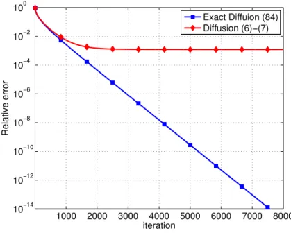
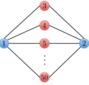
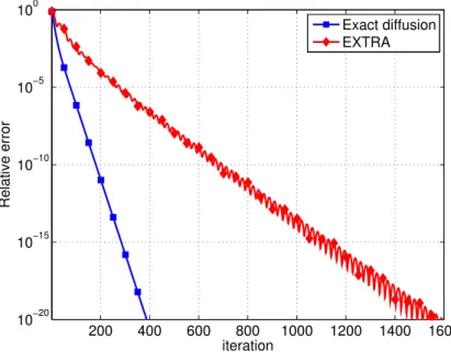
standard diffusion strategy. It turns out that diffusion relies on reformulating the aggre-gate optimization problem (1.1) as a penalized problem and resorting to a diagonally-weighted incremental construction. Since the achieved penalized problem is just an ap-proximation to problem (1.1), diffusion can only converge to an approximate solution rather than the desired wo. We next develop the exact diffusion method that directly solves the real problem (1.1) and thus eliminates the limiting bias. We also show in this chapter that the exact diffusion method is applicable to locally-balanced left-stochastic combination matrices which, compared to the conventional doubly-stochastic matrix, are more general and able to endow the algorithm with faster convergence rate, more flexible step-size choices and better privacy-preserving properties. In particular, the simulation shows exact diffusion with a locally-balanced combination matrix converges much faster than the benchmark method EXTRA [74] using the doubly-stochastic matrix.
• Chapter 3. In this chapter, we examine the convergence and stability properties of exact diffusion in detail and establish its linear convergence rate. We also show that it has a wider stability range than the EXTRA [75] consensus solution even if both algorithms employ the same symmetric and doubly-stochastic combination matrices, meaning that it is stable for a wider range of step-sizes and can, therefore, attain faster convergence rates. Analytical examples and numerical simulations illustrate the theoretical findings.
• Chapter 4. While the convergence property of exact diffusion is studied when solving distributed deterministic optimization problems in Chapters 2 and 3, its performance under adaptation and online learning settings remains unclear. It is still unknown whether the bias-correction is necessary over adaptive networks. By studying exact diffusion and examining its steady-state performance under stochastic scenarios, this chapter provides affirmative results. It is proved that the correction step in exact diffusion leads to a better steady-state performance than standard diffusion strategies
under mild conditions. It is also analytically shown the superiority of exact diffusion becomes more evident over sparse or badly-connected network topologies such as line, cycle, grid, and many others. This chapter also explores situations where exact diffusion and diffusion do perform similarly. These conclusions will provide a guideline on how to employ exact diffusion effectively in various applications.
• Chapter 5. In this chapter we extend exact diffusion to the empirical learning scenario with finite data samples. The problem considered in this chapter is more general than (1.4) in which the amount of data observed/collected by the individual agents may differ drastically, i.e., it is possible that Lk 6= L` for different agents k and `. To
guarantee linear convergence to the exact solutionwo, we integrate exact diffusion with an amortized variance-reduced gradient (AVRG) algorithm developed in [76]. AVRG is a stochastic variance-reduced method. Its memory cost is trivial compared to SAGA and it has a balanced gradient computations in comparison to SVRG. These two key advantages enable AVRG amenable to decentralized implementations. The resulting diffusion-AVRG algorithm is shown to have linear convergence to the exact solution which is opposed to the diffusion strategy that just converges to the neighborhood, see equation (1.25). Diffusion-AVRG is also shown much more memory efficient than the other alternative algorithms such as DSA [77]. In addition, we propose a mini-batch strategy to balance the communication and computation efficiency for diffusion-AVRG. When a proper batch size is selected, it is observed in simulations that diffusion-AVRG is more computationally efficient than exact diffusion or EXTRA while maintaining almost the same communication efficiency.
• Chapter 6. This chapter will summarize all derived results in the dissertation and discuss future work on exact diffusion learning.
1.4
Notation
Throughout the dissertation we use diag{x1,· · · , xK}to denote a diagonal matrix consisting
of diagonal entries x1,· · · , xR, and use col{x1,· · · , xR} to denote a column vector formed
by stacking x1,· · · , xR. For symmetric matrices X and Y, the notation X ≤ Y or Y ≥ X
denotes Y −X is positive semi-definite. For a vector x, the notation x 0 denotes that each element of x is non-negative, while the notation x 0 denotes that each element of x
is positive. For a matrix X, we let range(X) denote its range space, and null(X) denote its null space. The notation 1K = col{1,· · · ,1} ∈RK.
CHAPTER 2
Exact Diffusion for Distributed Optimization:
Algorithm Development
2.1
Context and Background
This chapter deals with deterministic optimization problems where a collection of K net-worked agents operate cooperatively to solve an aggregate optimization problem of the form:
w? = arg min w∈RM J?(w) = K X k=1 qkJk(w). (2.1)
In this formulation, each risk functionJk(w) is convex and differentiable, while the aggregate
cost J(w) is strongly-convex. Note that problem (2.1) is more general than the original problem (1.1). The weights {qk}Kk=1 are given positive constants to scale each local cost
function. When q1 = · · ·=qK = 1/K, problem (2.1) is equivalent to (1.1). All agents seek
to determine the unique global minimizer, w?, under the constraint that agents can only communicate with their neighbors. This distributed approach is robust to failure of links and/or agents and scalable to the network size. Optimization problems of this type find applications in a wide range of areas, see the discussion in Sec. 1.1.1.
2.1.1 Related Work
Research in distributed optimization dates back several decades (see, e.g., [70] and the ref-erences therein). In recent years, various centralized optimization methods such as (sub-)gradient descent, proximal gradient descent, (quasi-)Newton method, dual averaging, al-ternating direction method of multipliers (ADMM), and many other primal-dual methods have been extended to the distributed setting. In this section, we review several classes of
distributed algorithms that can be used to solve problem (1.1).
2.1.1.1 Distributed Primal Methods
In the primal domain, implementations that are based on gradient-descent methods are effective and easy to implement. There are at least two prominent variants under this class: the consensus strategy [5–13] and the diffusion strategy [1,4,34,36,71]. A brief description of these two primal strategies is given in Appendix 2.A. There is a subtle but critical difference in the order in which computations are performed under these two strategies. In the consensus implementation, each agent runs a gradient-descent type iteration, albeit one where the starting point for the recursion and the point at which the gradient is approximated are not identical. This construction introduces an asymmetry into the update relation, which has some undesirable instability consequences (described, for example, in Secs. 7.2–7.3, Example 8.4, and also in Theorem 9.3 of [1] and Sec. V.B and Example 20 of [4]). The diffusion strategy, in comparison, employs a symmetric update where the starting point for the iteration and the point at which the gradient is approximated coincide. This property results in a wider stability range for diffusion strategies [1, 4]. Still, when sufficiently small step-sizes are employed to drive the optimization process, both types of strategies (consensus and diffusion) are able to converge exponentially fast, albeit only toan approximate solution [1, 9]. Specifically, it is proved in [1, 9, 14] that both the consensus and diffusion iterates under constant step-size learning converge towards a neighborhood of square-error sizeO(µ2)
around the true optimizer, w?, i.e., kw? −wk,ik2 = O(µ2) as i → ∞, where µ denotes the
step-size and wk,i denotes the local iterate at agent k and iteration i. This limiting O(µ2)
bias is not due to any gradient noise arising from stochastic approximations; it is instead due to the inherent structure of the consensus and diffusion updates as clarified in the sequel.
Second-order information such as the Hessian matrix can also be introduced to the pri-mal methods, see the distributed Newton method [78, 79], Quasi-Newton method [80] and references therein. While the Hessian matrix helps accelerate the convergence rate, these second-order algorithms still suffer from the O(µ2) inherent limiting bias. There is another
type of methods that employ multi-consensus inner loop [81–83] and thus improves the con-sensus of the variables at each outer iteration. While these two-time scale methods can reduce the limiting bias, the inner consensus loop incurs more communication rounds be-tween agents, and hence slows down the processing of new data received in the outer loop. For this reason, they are not well-suited for the adaptation and online learning problems.
2.1.1.2 Distributed Primal-Dual Methods
Another important class of distributed algorithms are based on the primal dual strategies. A brief analytical derivation of various popular primal-dual methods is given in Sec. 2.B. A well-known family of distributed primal dual methods are those based on alternating direction method of multipliers (ADMM) [74, 84–86] and its variants [87–90]. In particular, work [74] proves that distributed ADMM with constant parameters converges exponentially fast to the exact global solution w?, which is in contrast to the purely primal methods we discussed in
Sec. 2.1.1.1 that only converge to an approximate solution close to w? with constant step-sizes. However, distributed ADMM solutions are computationally more expensive since they necessitate the solution of optimal sub-problems at each iteration. Some useful variations of distributed ADMM [87–89] may alleviate the computational burden, but their recursions are still more difficult to implement than consensus or diffusion due to their primal dual structures.
In more recent work [75, 91], a modified implementation of consensus iterations, referred to as EXTRA, is proposed and shown to converge to the exactminimizer w? rather than to anO(µ2)−neighborhood aroundw?. The modification has a similar computational burden as
traditional consensus and is based on adding a step that combines two prior iterates to remove bias. While EXTRA does not explicitly employ a dual variable, it is essentially a primal dual saddle point algorithm [77]. Motivated by [75], other variations with similar properties were proposed in [92–98]. These variations rely instead on combining inexact gradient evaluations with a gradient tracking technique. The resulting algorithms, compared to EXTRA, have two information combinations per recursion, which doubles the amount of communication
variables compared to EXTRA, and can become a burden when communication resources are limited. Distributed primal-dual second-order methods are also studied in [89, 99] to reduce communication rounds but they suffer from the expensive construction of the Hessian matrix. Due to their easy implementations and fast convergences, EXTRA and tracking methods have been extended to other important scenarios for directed [93, 97, 98, 100, 101] and asynchronous [102] networks. There is also another family of primal-dual methods that are related to EXTRA and utilize the network structure to further accelerate the convergence and reduce the communication rounds [103–105].
When local cost function Jk(w) is not smooth and has the structure Jk(w) = sk(w) +
rk(w) where sk(w) is smooth with Lipschitz continuous gradients and rk(w) is a possibly
non-smooth regularization term, one can integrate the proximal gradient descent with the above primal-dual methods, see [88, 91, 106–109]. In particular, [109] proposes a distributed proximal gradient method that endows with exponential convergence tow? when each agent
shares the same regularization term , i.e., r1(w) =· · ·=rK(w) = r(w).
2.1.1.3 Distributed dual methods
A third class of distributed algorithms are purely dual methods, see [110–113]. A short description on dual methods is provided in Sec.2.C. They first derive the unconstrained dual problem of problem (2.1) and then solve it by gradient descent. In particular, the algorithms of [110,111,113] can reach the optimal convergence rate by introducing Nesterov’s acceleration to their recursions.
2.1.2 Motivation and Contributions
The current chapter is motivated by the following considerations. The result in [75] shows that the EXTRA technique resolves the bias problem in consensus implementations. How-ever, it is known that traditional diffusion strategies outperform traditional consensus strate-gies. Would it be possible then to correct the bias in the diffusion implementation and attain an algorithm that is superior to EXTRA (e.g., an implementation that is more stable than
EXTRA)? This is one of the contributions in Chapter 2 and 3. In this chapter, we shall indeed develop a bias-free diffusion strategy that will be shown in chapter 3 to have a wider stability range than EXTRA consensus implementations. Achieving these objectives is chal-lenging for several reasons. First, we need to understand the origin of the bias in diffusion implementations. Compared to the consensus strategy, the source of this bias is different and still not well understood. In seeking an answer to this question, we will initially observe that the diffusion recursion can be framed as an incremental algorithm to solve a penalized version of (2.1) and not (2.1) directly — see expression (2.71) further ahead. In other words, the local diffusion estimate wk,i, held by agent k at iteration i, will be shown to approach
the solution of a penalized problem rather than w?, which causes the bias.
We have four main contributions in this chapter and the accompanying chapter 3 relating to: (a) developing a distributed algorithm (which we refer to as exact diffusion) that ensures exact convergence based on the diffusion strategy; (b) showing that exact diffusion has wider stability range and enhanced performance than EXTRA [75]; (c) showing that exact diffusion works for the larger class of locally balanced (rather than only doubly-stochastic) matrices; and (d) showing that neither EXTRA nor exact diffusion can be extended to the general directed network by constructing counter examples, which helps illustrate the significance of the proposed locally balanced conditions.
More specifically, we will first show in this chapter how to modify the diffusion strategy such that it solves the real problem (2.1) directly. We shall refer to this variant as exact diffusion. Interestingly, the structure of exact diffusion will turn out to be very close to the structure of standard diffusion. The only difference is that there will be an extra “correc-tion” step added between the usual “adapta“correc-tion” and “combina“correc-tion” steps of diffusion — see the listing of Algorithm 1 further ahead. It will become clear that this adapt-correct-combine (ACC) structure of the exact diffusion algorithm is more symmetric in comparison to the EXTRA recursions. In addition, the computational cost of the “correction” step is trivial. Therefore, with essentially the same computational efficiency as standard diffusion, the exact diffusion algorithm will be able to converge exponentially fast to w? without any bias. Secondly, we will show in Chapter 3 that exact diffusion has a wider stability range
than EXTRA. In other words, there will exist a larger range of step-sizes that keeps exact diffusion stable but not the EXTRA algorithm. This is an important observation because larger values for µhelp accelerate convergence.
Our third contribution is that we will derive the exact diffusion algorithm, and establish its convergence property for the class oflocally balancedcombination matrices (see Definition 1). This class does not only include symmetric doubly-stochastic matrices as special cases, but it also includes a range of widely-used left-stochastic policies as explained further ahead. First, we recall that left-stochastic matrices are defined as follows. Leta`k denote the weight
that is used to scale the data that flows from agent ` to k. Let A = [∆ a`k] ∈RK×K denote
the matrix that collects all these coefficients. The entries on each column of A are assumed to add up to one so that A is left-stochastic, i.e., it holds that
AT1K =1K, or K X
`=1
a`k= 1, ∀k = 1,· · · , K. (2.2)
The matrix A will not be required to be symmetric. For example, it may happen that
a`k 6=ak`. Using these coefficients, when an agent k combines the iterates {ψ`,i} it receives
from its neighbors, that combination will correspond to:
wk,i+1 = K X `=1 a`kψ`,i, where K X `=1 a`k = 1. (2.3)
Obviously, wk,i+1 is a convex combination of {ψ`,i}.
It should be emphasized that condition (2.2), which is repeated in (2.3), is different from all previous algorithms studied in [5, 74, 75, 84, 85, 88, 95, 96], which require A to be symmetric and doubly stochastic (i.e., each of its columns and rows should add up to one). For undirected networks, although symmetric doubly-stochastic matrices are commonly used, balanced left-stochastic policies can have significant practical value — they can speed up con-vergence, a more relaxed selection of the step-size parameter, reach better mean-square-error (MSE) performance over adaptive networks, and enjoy better privacy-preserving properties — see the extended discussions in Sec. 2.2.3.
We also explain in this chapter the significance of the proposed locally balanced condi-tions. If the combination matrix does not satisfy these conditions, we show that one can
construct counter examples where both exact diffusion and EXTRA diverge for any given step-size (see Sec. 2.5). This implies an interesting conclusion: exact diffusion and EXTRA may not always work for generaldirectednetworks (see the discussions in Secs. 2.2.4 and 2.5). This seems to be a disadvantage in comparison with DIGing-based methods [92–96] which are designed for directed network. However, for scenarios where the locally balanced condi-tion is satisfied, exact diffusion is shown in simulacondi-tions to have a wider range of step-sizes and is more communication efficient than DIGing methods [92–96] (recall that in DIGing there are two information combinations per iteration).
In this chapter we derive the exact diffusion algorithm, while in next chapter we establish its convergence properties and prove its stability superiority over the EXTRA algorithm. This article is organized as follows. In Sec. 2.2 we review the standard diffusion algorithm, introduce locally-balanced left-stochastic combination policies, and establish several of their properties. In Sec. 2.3 we identify the source of bias in standard diffusion implementations. In Sec. 2.4 we design the exact diffusion algorithm to correct for the bias. In Sec.2.5 we illustrate the necessity of the locally-balanced condition on the combination policies by showing that divergence can occur if it is not satisfied. Numerical simulations are presented in Sec. 3.3.
2.2
Diffusion and Combination Policies
2.2.1 Standard Diffusion StrategyTo solve problem (2.1) over aconnectednetwork of agents, we consider the standard diffusion strategy [1, 4, 34]:
ψk,i=wk,i−1−µk∇Jk(wk,i−1), (2.4) wk,i=
X
`∈Nk
a`kψ`,i, (2.5)
where {µk}K
k=1 are positive step-sizes. Compared to the diffusion method we present i
Al-gorithm 1.1, Recursions (2.4)–(2.5) employ different local step-size µk for each agent k.
the weighted consensus problem in (2.1). Moreover, in this chapter we will consider using a more relaxed combination policy in diffusion than the symmetric and doubly-stochastic matrix used in Sec. 1.2. Specifically, we assume {a`k}K`=1,k=1 are nonnegative combination
weights satisfying
X
`∈Nk
a`k = 1. (2.6)
It follows from (2.6) that A = [a`k] ∈ RK×K is a left-stochastic matrix, i.e., AT1K = 1K.
Note that we do not assumeAis symmetric here. The benefits of left-stochastic combination matrix over symmetric and doubly stochastic matrix is discussed in Sec. 2.2.3.
It is assumed that the graph is strongly-connected in this chapter, which means that at least one diagonal entry of Ais non-zero [1] (this is a reasonable assumption since it simply requires that at least one agent in the network has some confidence level in its own data). In this case, the matrix A will be primitive. This implies, in view of the Perron-Frobenius theorem [1, 114], that there exists an eigenvector p satisfying
Ap=p, 1TKp= 1, p0. (2.7)
We refer to p as the Perron eigenvector of A. Next, we introduce the vector
q = col∆ {q1, q2, . . . , qK} ∈RK, (2.8)
where qk is the weight associated with Jk(w) in (2.1). Let the constant scalar β be chosen
such that
q=βdiag{µ1, µ2,· · · , µK}p. (2.9)
whereβ >0 is some constant, then it was shown by Theorem 3 in [14] that under (2.9), the iterates wk,i generated through the diffusion recursion (1.5)-(1.6) will approach w?, i.e.,
lim sup
i→∞
kw?−wk,ik2 =O(µ2max), ∀k = 1,· · · , K, (2.10)
where µmax = max{µ1,· · · , µK}. Result (2.10) implies that the diffusion algorithm will
converge to a neighborhood around w?, and that the square-error bias is on the order of
O(µ2
max). We discuss a simple example in Sec.2.2 that justifies the existence of the inherent
Remark 2.1 (Scaling) Condition (2.9) is not restrictive and can be satisfied for any left-stochastic matrix A through the choice of the parameter β and the step-sizes. Note that β
should satisfy β = qk pk 1 µk (2.11) for all k. To make the expression for β independent of k, we parameterize (select) the step-sizes as µk = qk pk µo (2.12)
for some small µo > 0. Then, β = 1/µo, which is independent of k, and relation (2.9) is
satisfied.
Remark 2.2 (Perron entries) Expression (2.12) suggests that agent k needs to know the Perron entry pk in order to run the diffusion strategy (2.4)–(2.5). As we are going to see in
the next section, the Perron entries are actually available beforehand and in closed-form for several well-known left-stochastic policies (see, e.g., expressions (2.17), (2.21), and (2.26) further ahead). For other left-stochastic policies for which closed-form expressions for the Perron entries may not be available, these can be determined iteratively by means of the power iteration — see, e.g., the explanation leading to future expression (2.37).
2.2.2 Combination Policy
Result (2.10) is a reassuring conclusion: it ensures that the squared-error is small whenever
µmax is small; moreover, the result holds forany left-stochastic matrix. Moving forward, we
will focus on an important subclass of left-stochastic matrices, namely, those that satisfy a mild local balancecondition (we shall refer to these matrices as balanced left-stochastic poli-cies) [115]. The balancing condition turns out to have a useful physical interpretation and, in addition, it will be shown to be satisfied by several widely used left-stochastic combination policies. The local balance condition will help endow networks with crucial properties to ensure exact convergence to w? without any bias. In this way, we will be able to propose
distributed optimization strategies with exact convergence guarantees for this class of left-stochastic matrices, while EXTRA [75] is limited to (the less practical) doubly-left-stochastic policies; balanced left-stochastic matrices have many benefits as explained before, which is the main motivation for focusing on them in our treatment.
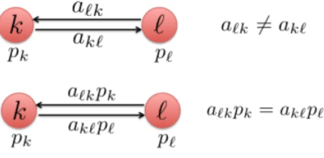
Definition 1 (Locally balanced Policies) Letpdenote the Perron eigenvector of a prim-itive left-stochastic matrix A, with entries {p`}. Let P =diag(p) correspond to the diagonal
matrix constructed from p. The matrix A is said to satisfy a local balance condition if it holds that
a`kpk =ak`p`, k, `= 1,· · ·, K (2.13)
or, equivalently, in matrix form:
P AT=AP. (2.14)
Relations of the form (2.13) are common in the context of Markov chains. They are used there to model an equilibrium scenario for the probability flux into the Markov states [116, 117], where the{a`k}represent the transition probabilities from states ` tok and the{p`}denote
the steady-state distribution for the Markov chain.
We provide here an interpretation for (2.13) in the context of multi-agent networks by considering two generic agents, k and `, from an arbitrary network, as shown in Fig. 2.1. The coefficient a`k is used by agent k to scale information arriving from agent`. Therefore,
this coefficient reflects the amount of confidence that agentk has in the information arriving from agent `. Likewise, for ak`. Since the combination policy is not necessarily symmetric,
it will hold in general thata`k 6=ak`. However, agent k can re-scale the incoming weight a`k
bypk, and likewise for agent `, so that the local balance condition (2.13) requires each pair
of rescaled weights to match each other. We can interpret a`k to represent the (fractional)
amount of information flowing from ` to k and pk to represent the price paid by agent k
for that information. Expression (2.13) is then requiring the information-cost benefit to be equitable across agents.
Figure 2.1: Illustration of the local balance condition (2.13).
It is worth noting that the local balancing condition (2.13) is satisfied by several important left-stochastic policies, as illustrated in four examples below. Thus, let τk = µk/µmax for
agent k. Then condition (2.9) becomes
q=βµmaxdiag{τ1, τ2,· · · , τK}p, (2.15)
where τk ∈(0,1].
Policy 1 (Hastings rule) The first policy we consider is the Hastings rule. Given {qk}N k=1 and {µk}Nk=1, we select a`k as [1, 118]: a`k = µk/qk max{nkµk/qk, n`µ`/q`} , if `∈ Nk\{k}, 1− X m∈Nk\{k} amk, if `=k, 0, if ` /∈ Nk. (2.16) where nk ∆
= |Nk| (the number of neighbors of agent k). It can be verified that A is
left-stochastic, and that the entries of its Perron eigenvectorp are given by
pk ∆ = qk/µk PK `=1q`/µ` >0. (2.17) Let β = K X `=1 q`/µ` = 1 µmax K X `=1 q`/τ` >0. (2.18)
With (2.16) and (2.17), it is easy to verify that
a`kpk =
1
βmax{nkµk/qk, n`µ`/q`}
If`=k, it is obvious that (2.13) holds. If` /∈ Nk, then k /∈ N`. In this case,a`kpk =ak`p` =
0.
Furthermore, we can also verify that when {qk}Nk=1 and {µk}Nk=1 are given, {a`k} are
generated through (2.16), and β is chosen as in (2.18), then condition (2.9) is satisfied.
Policy 2 (Averaging rule) The second policy we consider is the popular average combi-nation rule wherea`k is chosen as
a`k = 1/nk, if ` ∈ Nk, 0, otherwise. (2.20)
The entries of the Perron eigenvector p are given by
pk =nk K X m=1 nm !−1 . (2.21)
With (2.20) and (2.21), it clearly holds that
a`kpk = K X m=1 nm !−1 =ak`p`, (2.22) which implies (2.13).
We can further verify that when µk is set as
µk =
qk
nk
µo, ∀k = 1,2,· · · , N (2.23)
for some positive constant step-size µo and β is set as
β = K X m=1 nm ! . µo >0, (2.24)
then condition (2.9) will hold.
Policy 3 (Relative-degree rule) The third policy we consider is the relative-degree com-bination rule [119] where a`k is chosen as
a`k = n` Pm∈Nknm −1 , if `∈ Nk, 0, otherwise, (2.25)
and the entries of the Perron eigenvector p are given by pk= nkPm∈Nknm PK k=1 nk P m∈Nknm . (2.26)
With (2.25) and (2.26), it clearly holds that
a`kpk= nkn` PK k=1 nk P m∈Nknm =ak`p`, (2.27) which implies (2.13).
We can further verify that when µk is set as
µk= qk nk P m∈Nknm µo, ∀k = 1,2,· · · , K, (2.28) and β is set as β = K X k=1 nk X m∈Nk nm ! . µo, (2.29)
then condition (2.9) will hold.
Policy 4 (Doubly stochastic policy) If matrix A is primitive, symmetric, and doubly stochastic, its Perron eigenvector is p= K11K. In this situation, the local balance condition
(2.13) holds automatically.
Furthermore, if we assume each agent employs the step-sizeµk=qkKµo for some positive
constant step-size µo, it can be verified that condition (2.9) holds with
β = 1/µo. (2.30)
There are various rules to generate a primitive, symmetric and doubly stochastic matrix. Some common rules are the Laplacian rule, maximum-degree rule, Metropolis rule and other
rules that listed in Table 14.1 in [1].
Policy 5 (Other locally-balanced policies) For other left-stochastic-policies for which closed-form expressions for the Perron entries need not be available, the Perron eigenvector