Volume 55, 2018, Pages 243–255
GCAI-2018. 4th Global Conference on Artificial Intelligence
Replaceability for Constraint Satisfaction Problems:
Algorithms, Inferences, and Complexity Patterns
Richard J. Wallace
Insight Centre for Data Analytics
Department of Computer Science, University College Cork, Cork, Ireland [email protected]
Abstract
Replaceability is a form of generalized substitutability whose features make it potentially of great importance for problem simplification. It differs from simple substitutability in that it only requires that substitutable values exist for every solution containing a given value without requiring that the former always be the same. This is the most general form of substitutability that allows inferences from local to global versions of this property. Building on earlier work, this study first establishes that algorithms for localized replaceability (consistent neighbourhood replaceability or CNR algorithms) based on all-solutions neighbourhood search outperform other replaceability algorithms by several orders of magnitude. It also examines the relative effectiveness of different forms of depth-first CNR algorithms. Secondly, it demonstrates an apparent complexity ridge, which does not occur at the same place in the problem space as the complexity areas for consistency or full search algorithms. Thirdly, it continues the study of methods for inferring replaceability in structured problems in order to improve efficiency. Here, it is shown that some strategies for inferring replaceable values can be extended to disjunctive constraints in scheduling problems.
1
Introduction
Among the many methods devised for simplifying constraint satisfaction problems, those based on substitutability form a significant class. In contrast to methods that discover and remove inconsistent values, i.e. values that cannot appear in any solution, substitutability methods remove values that may be perfectly viable. However, in these cases other viable values can be substituted for the value removed without affecting the validity of the solution. Hence, removal depends on the fact that these values are redundant with respect to problem satisfiability.
As with consistency methods, there is now a body of work concerned with specifying various forms of substitutability as well as related properties such as interchangeability or mutual substitutability. A useful summary of this work is found in [10]. One of the most interesting developments in this area is the demonstration that generalized forms of substitutability can be defined that effectively loosen the criteria for value removal without affecting the guarantee that, given a solution with those values, other solutions can still be found [8,1,6].
within that hierarchy a particular form of generalized substitutability has certain maximal features that make it of great potential interest. Bordeaux and co-workers called this property “removability”. How-ever, this term can lead to confusion with a still more general property called “dispensability” [4], so it seems best to use a different and perhaps more apposite term. For this purpose, we have chosen the term “replaceability”, which seems to have exactly the right connotations.
Perhaps the most important feature of replaceability is that it is the most general form of substi-tutability that supports local to general reasoning. Unfortunately, as shown earlier and discussed below, this does not give us a form of the property that is tractable, in contrast to simple substitutability (or local consistency). Nonetheless, earlier work has shown that algorithms for local forms of replaceability can be devised that are feasible for some problems [6].
Building from the results reported in [6], the present work extends the analysis of this property. In the first place, we consider other algorithms that have been proposed in recent years to determine whether they are reasonable alternatives to the algorithms we devised. Then we examine a potentially significant critical complexity effect found with replaceability algorithms. Although it is based on a dynamics that is similar to the well-known phase transition, involving a tradeoff between number of possible tuples and a decreasing likelihood that any one of them will be viable, it does not involve a phase transition. Finally, we extend earlier work on inferring replaceability to the important class of scheduling problems with disjunctive constraints.
In the past, there have been a few efforts in this direction. The earliest is the work by Jeavons et al., who defined what they called “generalized substitutability” [8]. Later Bordeaux et al. defined a similar but simpler concept that they called “removability” [1], which is identical to replaceability as we define it here. Then Freuder showed that replaceability could support certain forms of local to global reasoning [4]. Subsequently, Likitvivatanavong and Yap discussed the same idea and proposed a new algorithm for removing all replaceable values [11]. As noted above, Freuder and Wallace recently delineated a “substitutability hierarchy” and showed that replaceability is the most general property in this hierarchy that can support local to global reasoning. These authors also proposed two new algorithms for local replaceability based on depth-first search [6].
2
Background and Basic Concepts
A constraint satisfaction problem (CSP) involves choosing values for a set of variables,X, which satisfy a set of constraints, C, each of which specifies permissible combinations of values for a subset of the variables. Each value selected for variableXi must come from a domain of valuesDi associated
with that variable. A choice of values for a subset,S, of the variables is an instantiation ofS. If the instantiation is consistent with constraints based on variables inS, then we say that itsatisfies those constraints. An instantiation of all the variables,X, which satisfies all the constraints in the problem is a solution.
CSPs can be simplified by removing values that are “inconsistent”, i.e. that cannot appear together with any value in any solution. In addition, simplification can be effected if whenever a value appears in a solution, another value can be found to substitute for it without making the solution invalid.
The basic property of substitutability in CSPs was first characterised in [3]. Here, we will use an equivalent definition that corresponds to later definitions in which the focus is on the value discarded.
Definition 1. Given a value v in domainDi of variable Xi, if for any solution in whichv appears,
we can substituteuand still have a solution, thenv has the property ofsubstitutabilityand valueuis substitutable forv.
toXiin the constraint graph. These are the variables that share a constraint withXi.
Definition 2.(From [3]) For two valuesuandvbelonging to the domain of variableXi,uis
neighbour-hood substitutableforviff for every constraint onXi, ifvsatisfies the constraint thenualso satisfies it.
This latter property had two important features: (i) neighbourhood substitutability is sufficient (but not necessary) for full substitutability, (ii) neighbourhood substitutability can be determined in polyno-mial time.
As already noted, an important generalization of substitutability holds when for a given valuevwe can substitute some value, not necessarily unique, in any solution in whichvappears. This property we call replaceability. More formally,
Definition 3.(From [1]) An valuevisreplaceableif for any solution involvingv, there is some other instantiation that can be substituted forvand still have a solution.
In other words, a value is replaceable if some value can be found to substitute for it in any solution, and it is also substitutable if a single other value can be substituted for it ineverysolution. Thus, sub-stitutability implies replaceability, while replaceability does not imply subsub-stitutability. In other words, replaceability is a more general property since any values that can be removed on the basis of substi-tutability are also replaceable, but not vice versa.
While weaker and more general forms of substitutability can be defined, including minimal substi-tutability [6], these properties lack an important feature of the stronger properties. This is that up to and including replaceability, the property in question is defined with respect toallsolutions in which instan-tiationvappears, i.e. all solutions supported by a replaceable valuevare still supported. In particular, in [6] it was shown that:
Proposition 1. Replaceability is the most general form of substitutability for which all solutions con-sistent with a discarded value are concon-sistent with some remaining value.
It can therefore be said that replaceability is a “maximal property” with respect to this feature.
In this paper we will not consider generalizations of these properties that involvek-tuples of values withk >1and which can involve sets of values or tuples to be replaced. This is because they entail complexities in computation and representation that will make it difficult to use them in practice. In particular, as shown in [6], substitutability in terms ofk-tuples over a variable setR does not imply that individual values in the set are substitutable. In other words, the property of substitutability when applied to ak-tuple is not decomposable.
Removing instantiations based on these properties, either in preprocessing or dynamically during search, can reduce search effort. In general, however, determining various forms of substitutability can be as intractable as solving the original problem. However just as with substitutability, for replaceability we can define local forms that imply full replaceability (see [6] for proofs). Here, we will focus on the simplest and most useful form that we call neighbourhood replaceability.
Definition 4. An instantiation of a single variableXiisneighbourhood replaceableif it is replaceable
with respect to the subgraph formed byXiand all variables that share a constraint withXi.
Unfortunately, in contrast to substitutability, the complexity of even the local form of replaceability is non-polynomial. Nonetheless, there are cases where such computations are feasible. So we turn next to a consideration of algorithms for this task.
3
Neighbourhood Replaceability Algorithms
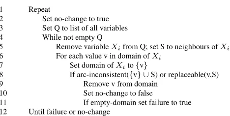
1 Repeat
2 Set no-change to true 3 Set Q to list of all variables 4 While not empty Q
5 Remove variableXifrom Q; set S to neighbours ofXi
6 For each value v in domain ofXi
7 Set domain ofXito{v}
8 If arc-inconsistent({v} ∪S) or replaceable(v,S) 9 Remove v from domain
10 Set no-change to false
11 If empty-domain set failure to true 12 Until failure or no-change
Figure 1: CNR-1 algorithm for neighbourhood replaceability.
1 Set Q to list of all variables 2 While not empty Q and not failure
3 Remove variableXifrom Q; set S to neighbours ofXi
4 For each value v in domain ofXi
5 Set domain ofXito{v}
6 If arc-inconsistent({v} ∪S) or replaceable(v,S) 7 Remove v from domain
8 If empty domain set failure to true
9 Else put neighbours ofXiin Q if not there already
Figure 2: CNRQ algorithm for neighbourhood replaceability.
analogous to the local computation of neighbourhood inverse consistency [5]. The second approach de-pends heavily on inferences about the number of neighbourhood tuples associated with a given value and the number available to replace it. This is exemplified by the algorithm described by Likitvivatanavong and Yap [11].
In this section we briefly descibe the two neighbourhood search algorithms that were introduced in [6]. (There one can find soundness proofs for these algorithms.) These algorithms are designated as “consistent neighbourhood replaceability” (CNR) algorithms because they remove all values that are locally replaceable including arc-inconsistent values. In this form neighbourhood replaceability subsumes (and therefore dominates with respect to value removal) neighbourhood consistency algo-rithms such as neighbourhood inverse consistency (NIC) and neighbourhood singleton arc consistency (NSAC). Briefly, NIC establishes that a valuev of variable Xi is consistency with at least one tuple
based onXiand its neighbours, while NSAC determines whether the neighbourhood subgraph can be
made arc consistent whenvis the only member of the domain ofXi. (See [5,13] for more detailed
discussion.) In addition, we describe a slightly altered version of the Likitvivatanavong-Yap algorithm. (Another algorithm for generalized substitutability was proposed by [8], but since it is not oriented toward finding single replaceable values, and it seems fairly inefficient, it is not described here.)
The first CNR algorithm, CNR-1, uses an AC-1 style procedure in which all values in the problem are repeatedly tested for replaceability until no value is discarded. In the implementation of this algo-rithm, the replaceable procedure uses a MAC-style search (MAC=maintained arc consistency) to find all solutions for the subproblem, and for each solution it seeks a value from the current domain that can replace valuev. Pseudocode for this algorithm is shown in Figure1. The second algorithm, CNRQ, uses a queue updating mechanism in place of the repeat loop used by CNR-1. Pseudocode for this algorithm is shown in Figure2.
1 Set up merge tables for entire problem 2 Set Q to list of all variables
3 While not empty Q
4 Remove variableXifrom Q; set S to neighbours ofXi
5 For each value v in domain ofXi
6 Establish neighbourhood inverse consistency 7 If any merge list is singleton v % value is irreplaceable
8 continue
9 goal-count←tuples 10 ub-count←tuples
11 If ub-count<goal-count % value is irreplaceable
12 continue
13 Choose any constraint onXi
14 While potential tuples remain
15 Form next tuple that can replace v from merge-lists 16 and save if not already in store
17 If —tuples in store— = goal-count 18 remove value and continue
19 If values removed return missing neighbours ofXito Q
Figure 3: Likitvivatanavong-Yap (LY) algorithm for neighbourhood replaceability embedded within a top-level AC-3 style queue.
was used for handling the entire problem. In addition NIC was substituted for the maxRPC algorithm in the original description; this made the present algorithm more comparable to the other algorithms. Pseudocode for this algorithm is shown in Figure3.
The algorithm begins with some initialization steps. The most elaborate is the setting up ofmerge tablesfor each variable in the problem. Here, we will consider only problems with binary constraints. 1 In this case, the tables for each variableX
icontain the values in the domain ofXithat are supported
by each value in the domain of each adjacent variable. Suppose, for example, thatXi has only one
neighbourXj, that each variable has three values, and the constraint is an inequality constraint. Then
the merge table would have the form, {2 3}1 {1 3}2 {1 2}3
where the values in brackets are those in the domain ofXithat go with the value in the domain ofXj,
which is indicated on the right. In this paper the values in brackets are calledmerge sets. (In practice, the latter value can be represented implicitly by an array index.)
In the main procedure, at each step a variable is taken off the queue and all values in its domain are checked for replaceability. Following removal of neighbourhood-inconsistent values (line 6), this algorithm carries out a series of steps, each of which determines if the value being tested is irreplaceable or replaceable. In the first test the merge sets are checked to determine if the present value is contained in a singleton; in this case, the value is irreplaceable. Prior to the next two tests, two values are computed: the number of neighbourhood tuples associated with the value being tested (goal-count) and the number of neighbourhood tuples associated with alternative values (ub-count). (In the merge table above for value 1 the goal-count is 2 and the ub-count is also 2.) Then, the next test checks whether the ub-count is less than the goal-count; if it is, then the value is irreplaceable. Finally, viable tuples are collected for
1
2
3
{a,b,c}
{a,b}
{a,b}
(aa) (ab) (ba) (ca) (cb)
(aa) (ab) (bb) (ca) (cb)
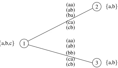
Figure 4: Example showing that more than one fixpoint is possible when all replaceable values are removed.(Domains are shown in brackets, satisfying constraint tuples are in parentheses.)
the values that could substitute for the value being tested; if ever their number equals the goal-count, then the value being tested is replaceable.
The final test is the most elaborate since it must calculate a union of tuples. In the present work two methods were tried. The first uses an array with dimensions Number-of-Adjacent-Variables X Domain-Size X Number-of-Tuples. Array entries are t or nil depending on whether or not thekth value in tuple
mhas value a. This allows fast checking, but can requireO(num−neighbourhood−tuples)tuple checks. The second method uses a trie structure in which if thekth value in tuplemhas valuea, then at that level the (domain size) array will point to another array representing the next value in the tuple (or ifais the last value, the array entry will have the value t). This allows for fast checking, although there is a proliferation of small arrays each time a value is checked for replaceability. Since the second method was found to improve performance by at least an order of magnitude, this was the version used in experimental tests.
Although replaceability algorithms terminate with a set of irreplaceable values, these sets can vary depending on the order of testing. In other words, replaceability algorithms do not have unique fixpoints. This can be shown by example, as in Figure4. In this problem, if we begin with variable 1 we can either replace valueawith{b, c}or vice versa. This will then yield different fixpoints.
4
Notes on Experimental Methods
As stated in our earlier work, higher-order properties such as replaceability will become more useful as the field moves away from one-shot problem solving to more long-term venues involving problem compilation and/or repeated solving in evolving situations. However, we can still learn something about the effects of establishing replaceability, as well as the costs in experiments involving preprocessing and then search on individual problems.
The present tests were carried out using three types of problems:
1. Heterogeneous random problems with “geometric” constraint graphs in which the probability of support was varied2,
2. Random distance problems, i.e. problems with constraints of the form|Xi−Xj|> k,
2As noted earlier, homogeneous random problems have few replaceable values except in domains of variables of very low
3. Random relop problems, i.e. problems with (binary) constraints based on relational operators, e.g.Xi> Xj. Problems included not-equals constraints to ensure intractability.
Geometric problems used in the main experiments had 120 or 300 variables, both with domain size 20. Constraint graphs were constructed using the procedure described in [9], which gives the graphs a ‘clumpy’ character. For 120 variables the (Euclidean) distance parameter was 0.17 and problems were filtered to allow only those with 540 constraints±3. For 300 variables the distance parameter was 0.1 and the number of constraints was 1320±5. There were two levels of support: for 70% of the values tightness (obverse of support) was 0.2; for 30% it was 0.8. Support for different adjacent variables was computed independently of other constraints.
Distance problems had 50 variables, domain size 10, constraint graph density 0.10, and fixedk= 3. Relop problems used in the main experiments had 40 variables, domain size 10, and constraint graph density = 0.60. Problems used in Section 7 had 30 variables, domain size 8 and varying constraint graph densities. All relop problems had>and<>constraints in equal proportions.
Samples of 50 problems were used except for 120-variable geometric problems where the sample size was 100. The parameter values used allowed samples of satisfiable and unsatisfiable problems to be generated in each case.
In these experiments search was done with MAC-3. For most problem sets the domain/forward degree variable ordering heuristic was used, while for 300-variable geometric problems the domain/ weighted degree heuristic of [2] was used.
In most tests, in addition to CNR algorithms, three other kinds of preprocessing were also performed: simple arc consistency, neighbourhood singleton arc consistency (NSAC), and neighbourhood inverse consistency (NIC). The comparisons of interest were runtimes and number of values removed.
5
Comparing the Three CNR Algorithms
The first set of tests was run to compare the all-solutions search algorithms with the Likitvivatanavong-Yap algorithm. This is important because of the very different strategies used in the two cases.
For reasons that will become evident, these experiments were run with very small problems. Random geometric problems were used with 20 variables, domain size ten, and a distance factor of 0.200. Two levels of support were used: 60% of the values had a support = 0.8, and the remaining 40% had a support of 0.2. Problems were filtered during generation so that, (i) all problems had 36±2 constraints, (ii) all problems had solutions. Fifty problems were tested.
CNR algorithms removed an average of 122 values our of 200, while AC removed 16 and both NSAC and NIC removed 34. Of much greater consequence are the runtimes. CNRQ required an average of 0.12 seconds per problem; CNR-1 was slightly slower at 0.16 seconds. (AC required<0.01 seconds, NSAC 0.03, NIC 0.06.) This was markedly different from CNR-LY, which required 30,382 seconds on average, so that the run for this algorithm could barely be finished.
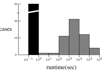
Further insight into the differences in runtime is obtained by considering individual runtimes, which are summarized in the frequency histogram shown in Figure5. To accomodate the large variation in a single figure, runtimes (in seconds) are binned according to successive powers of ten. As shown here, all 50 problems give runtimes less than one second when CNRQ is used (likewise for CNR-1), while for CNR-LY, runtimes are at least100seconds and are sometimes more than105.
0 10 20 50
10−1 100 101 102 103 104 105 106
cases
runtime(sec)
Figure 5: Frequency histogram for CNRQ (black) and CNR-LY (gray). Fifty problems in all. (Note log scale on abscissa.)
6
Comparing CNR-1 and CNRQ
For random geometric problems, CNR finds a large number of replaceable values, about 25% more than NIC, showing that it is effective in simplifying problems (see Table 1; because of space constraints only satisfiable problems are shown). For smaller problems, the reduction in subsequent search time actually compensates for the extra preprocessing time. (As a side note, it is also interesting to see how effective NIC alone was on these problems.) A similar pattern of results was found with unsatisfiable problems; in addition either NIC alone or CNR proved unsatisfiability in approximately 90% of the cases.
Table 1. Search Efficiency and Values Removed for Geometric Problems with Variable Support
satisfiable-120 satisfiable-300
rem nodes preproc search rem nodes preproc search
AC 39 46,265 0.1 266.2 95 7,917 0.2 258.3
NSAC 184 20,906 8.8 89.8 492 2,236 300.3 81.2
NIC 301 268 36.9 0.7 924 1,402 2304.4 45.4
CNR-1 370 269 149.6 0.7 – – – –
CNRQ 370 269 67.8 0.6 1148 1,451 5269.6 49.1
Notes. Means for values removed during preprocessing (rem), search nodes, preprocessing and search times (sec).
For the 300-variable problems, only partial results were collected with CNR-1 for both satisfiable and unsatisfiable problems. Runtimes exceeded CNRQ by up to five times depending on the problem, so that times of104 were observed. Hence, no attempt was made to use this algorithm on the entire problem set.
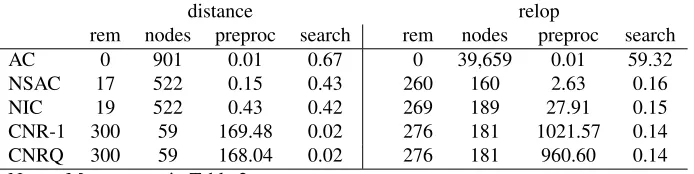
Table 2. Search Efficiency and Values Removed for Distance and Relop Problems
distance relop
rem nodes preproc search rem nodes preproc search
AC 0 901 0.01 0.67 0 39,659 0.01 59.32
NSAC 17 522 0.15 0.43 260 160 2.63 0.16
NIC 19 522 0.43 0.42 269 189 27.91 0.15
CNR-1 300 59 169.48 0.02 276 181 1021.57 0.14
CNRQ 300 59 168.04 0.02 276 181 960.60 0.14
Notes. Measures as in Table 2.
These tests show that many problem types are amenable to simplification by removing replaceable values. They also reaffirm the point made previously [6] that given the expense involved in carrying out these procedues, methods for inferring replaceability without search will be of critical importance.
7
Patterns of Difficulty Across the Problem Space
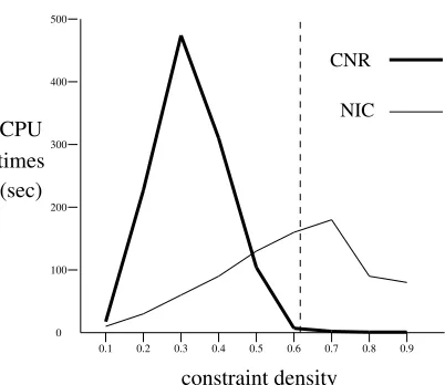
While testing neighbourhood replaceability algorithms, a pattern of effort as a function of problem pa-rameters was discovered that is remniscent of the well-known critical complexity effect for CSP search. An example is shown in Figure 6, where a curve for CNR runtime appears along with a corresponding curve for NIC. In this experiment, constraint density is the parameter that is varied. 3 As with other types of local consistency algorithms [7], the curve for NIC reaches its highest point near the phase transition. In contrast, the peak of the CNR curve is well to the left of this point in the “easy” region with respect to search effort. (Mean search effort following AC in terms of nodes was 106 at 0.5 density, 930 at 0.6, and 518 at 0.7, using min domain/forward-degree.)
Similar results were found with distance problems. With ‘geovarsat’ problems the results were not clear-cut, but in this case varying constraint density also changes patterns of connectivity (i.e. with more constraints the constraint graph becomes less clumpy); hence, it isn’t clear whether complexity effects like those found with other problem types should be found here as well.
To get some insight into the basis for this effect, tests were done on the same problems where various operations and other measures were counted, in particular number of neighbourhood solutions and queue additions. (Value removals were already counted.) While value deletions and queue additions did not show any clear relation to runtimes, there was a strong correlation with the number of neighbourhood solutions, as shown in Table 3.
Why are there so many neighbourhood solutions? With increasing density, neighbourhood size increases, and therefore the number of possible tuples grows asdk, wherekis the number of neighbors.
But at the same time the number of constraints among neighbours will also increase. Given a particular variable with neighbourhood of sizek, we can calculate the likelihood that an additional constraint will either produce a new neighbour or increase the number of constraints within the neighbourhood subgraph composed of the variable and its neighbours. The former isn1∗(n−nk−1)= (n−nk2−1), the latter
is(kn)2. For problems with 30 variables, and density = 0.1 (in terms of the proportion of edges added to a spanning tree), the average degree is 5. This, in turn, gives a probability of about 0.027 for adding a new neighbour and 0.028 for adding a constraint to the neighbourhood subgraph. For density = 0.3, the average degree is about 10, and the two probabilities are approximately 0.021 and 0.111, respectively. So we can see a shift in relatively likelihood between these two densities. By setting the two expressions
3In this case density is in terms of the edges added to a spanning tree. Thus all graphs are connected. This means that 0
0 100 200 300 400 500
0.1 0.2 0.3 0.4 0.5 0.6 0.7 0.8 0.9 CPU
times (sec)
constraint density
CNR
NIC
Figure 6: Runtime curves for CNRQ and NIC with relop problems of varying constraint density. Each point is the mean for 50 problems. Vertical dashed line indicates approximate transition (50:50) point from satisfiable to unsatisfiable problems.(Note. Runtimes for NIC were multiplied by 100 so its curve could be viewed on same scale as CNR.)
equal to each other, we can derive a value ofkequal to 5 for the crossover point for problems of this size.
Table 3. CNR Statistics for Relop Problems
density neigh-sols removals Q-addits prove unsol
0.1 297,025 193 99 –
0.2 3,889,129 101 67 –
0.3 9,564,750 82 57 –
0.4 6,706,596 95 58 –
0.5 1,809,104 122 72 1
0.6 72,054 152 70 17
0.7 2,236 79 20 44
0.8 5 14 1 50
0.9 – – – 50
Note. Same relop series as in Figure 6.
It might be argued that since there is no phase transition in this case, this cannot be considered a complexity peak. Although I can’t yet be certain that there is a genuine asympototic complexity effect, for some classes of problems (perhaps for random problems of the RB type), this may well be the case. The implication is that complexity peaks are a more general phenomenon than phase transitions. In fact, garden path based complexity (backtrack search algorithms), support path based complexity (inconsistency algorithms), and neighbourhood solution based complexity (CNR) share a basic property. All are related to a situation where the number of possibilities increases at the same time that the likelihood that a possibility is a viable member of the desired set is decreasing.
The present difficulty peak is obviously related to one that might be found for all-solutions search (depending on the problem model and manner of search). A significant difference is that, as shown in the table, the result obtained in this case (number of deletions) does not itself increase.
it was impossible to test certain structured problems beyond a very small number of variables, because on testing with increasing density I quickly came up against very long runtimes and had assumed that the situation would only get worse as density increased. Now we know that the limits are not quite as severe provided one stays away from the peak complexity areas.
Given that it is based on the requisite all-solutions search, it may be possible to ameliorate this effect by standard methods of checking for cycle breaking and then collecting cross-products of remaining domain values to be tested for replaceability. However, this has not yet been attempted.
8
Inferring Replaceability: Further Discussion
In our earlier paper we argued that for some structured problems it is possible to deduce replaceability of some of the values. In particular, for distance constraints of the form|Xi−Xj| ⊗kthat do not
involve equalities there are several ways to avoid checking individual values. First, depending on the minimal distance, it may be possible to infer substitutability for values near the extremes, since support for extreme values will always include the support for less extreme values. (Here, we will refer to these as subset inferences.) There are also symmetry relations with respect to support for values in the lower and upper halves of the range such that if a value in one half-range can be shown to be replaceable then its complement in the other half-range is also replaceable.
However, conditions must be met to ensure that the latter maneuver is valid. In previous work we did not include a proof of this technique, and in fact there was a minor flaw in the program. In this paper we present a proof, which involves the conditions under which this strategy will give valid results.
We first consider the simplest case in which all domains contain a complete sequence of integers, i.e. there are no breaks in the sequence, and constraints are all of the form|Xi−Xj|> k, i.e. there is
only onekvalue.
Proposition 2.For problems based on distance constraints with the properties just given, if a valuevis replaceable, then the symmetric valuen−v+ 1is also replaceable provided that there is a symmetrical set of values around the midpoint of the domain.
Proof. We assume that the initial domains are complete integer sequences between 1 andmifor each
variableXi. (The necessary property is that for each valuevbelow the midpoint, there is a valuen−v+1
above the midpoint.) Suppose we have found the first replaceable valuevfor a given variableXi. We
consider any set of replacement values. Since the domain is a complete sequence, for every replacement valuew, wherew−v=d, there will be a corresponding domain valuew0where the difference between
w0andn−v+ 1will also bed. In fact, if we addd
v−symm, the difference betweenvandn−v+ 1,
to any valuewwe obtain the correspondingw0.
Next, we consider the set of neighbourhood tuples supported by eithervorn−v+ 1, respectively. Note that the cardinality of these sets may differ depending on the neighbour domains. However, taking either set and some replacement set{w}or{w0}, the complementary set,{wcomp}or{w0comp}, will be
found in the domain ofXiby virtue of the symmetry of the domain. Hence, ifvis replaceable it will be
possible to replace the symmetrical valuen−v+ 1.
Now, suppose we have replacedkvalues in a domain, and the remaining values are symmetrical around the midpoint. Then by the same reasoning, if a valuevis shown to be replaceable, thenn−v+ 1
can also be replaced.2
This argument can be extended to constraints of the form|Xi−Xj|< k, or to corresponding forms
It is of particular interest that these arguments can be extended to problems with disjunctive con-straints of the same character, which includes scheduling problems. Here, the concon-straints usually have the formXi+k1 < Xj W Xj+k2 < Xi. The two components can be rewritten asXj−Xi > k1 andXi−Xj > k2, respectively. This, in turn, implies the constraint|Xi−Xj| > min(k1, k2). It follows that if for a given valuev all members of the replacement set satisfy the derived constraint, and the conditions specified in Proposition 9 also hold, then we can also replace the symmetrical value
n−v+ 1.
In this case, however, care must be taken to ensure that asymmetries are not introduced by incon-sistency processing. In the present work a very conservative procedure was used. (Whether there are more efficient procedures is an open question.) After each deletion, the symmetrical complement was the next value tested; if it was not inconsistent, then a symmetry flag for that domain was set to nil, and after that no inferences based on symmetrical values were attempted.
In earlier work with simple distance problems [6] we found that by using subset and symmetry inferences along with skipping replaceability checks for extreme values, we could reduce the time to find an irreplaceable set by three orders of magnitude, from104 to101 seconds. In the present work problems derived from the Taillard benchmarks were tested, specifically the os-taillard-4-100 set [12], which includes ten problems. Since even these problems had domains that were much too large to apply value-by-value tests, the domains were reduced to about a quarter of their original size, which is roughly from 200 to 50. (The resulting problems still had solutions.)
Despite this reduction, the basic CNRQ algorithm required an average of 30,000 seconds. A large portion of this effort was due to one problem that required 267,000 seconds to process. However, four other problems required104seconds, ranging from 10 to 36 thousand.
Using either subset or symmetry inferences alone reduced the mean to 16 and 14 thousand seconds, respectively. Using these methods together along with skipping the extreme values brought a further reduction to 8 thousand seconds. Moreover, for some problems it was possible to reduce the time from
104to102or101. So, while not finding the spectacular overall reduction obtained for simple distance problems, it was possible to bring about a clear reduction with these methods, which in some case was marked.
9
Conclusions and Future Work
This work has clarified some issues related to the important property of replaceability. In particular, we have determined what is presently the best algorithmic approach to finding a neighbourhood irreplace-able set, and we have corrected and clarified some questions in regard to inferring replaceability for constraints with certain kinds of structure.
In addition, we have discovered a new critical complexity region associated with neighbourhood replaceability algorithms and analyzed some of its features. This is of both theoretical and practical interest.
This work extends the general study of substitutability in connection with CSPs. Even more gener-ally, it contributes to the study of higher-level properties that can be used to simplify problems.
There are still many other topics that need to be considered. Most important, perhaps, is the use of replaceability in compilation techniques such as MDDs. The fact that there is no unique fixpoint raises several issues such as the existence of minimal sets of irreplaceable values and smallest minimal sets, although whether such sets can be found efficiently remains to be determined. Finally, it may be possible to find approximations to full replaceability that are almost as effective whilst being more efficient. In this connection, if the degree of the variables whose domains are tested for a property like replaceability is limited by a certain value, it may be possible to obtain a fixed-parameter tractable form of the property. Whether such variants are useful in practice is a question that must be decided in the future.
References
[1] L. Bordeaux, M. Cadoli, and T. Mancini. A unifying framework for structural properties of CSPs: Definitions, complexity, tractability.Journal of Artificial Intelligence Research, 32:607–629, 2008.
[2] F. Boussemart, F. Hemery, C. Lecoutre, and L. Sais. Boosting systematic search by weighting constraints. In Proc. Sixteenth European Conference on Artificial Intelligence-ECAI’04, pages 146–150. IOS, 2004. [3] E. C. Freuder. Eliminating interchangeable values in constraint satisfaction problems. InNineth National
Conference on Artificial Intellgence – AAAI’91, pages 227–233, 1991.
[4] E. C. Freuder. Dispensable instantiations in constraint satisfaction problems. InTenth International Workshop on Constraint Modelling and Reformulation – ModRef 2011, 2011.
[5] E. C. Freuder and C. D. Elfe. Neighborhood inverse consistency preprocessing. In Thirteenth National Conference on Artificial Intelligence – AAAAI’96. Vol. 1, pages 202–208. AAAI/MIT, 1996.
[6] E. C. Freuder and R. J. Wallace. Replaceability and the substitutability hierarchy for constraint satisfaction problems. In C. Lisetti C. Benzmueller and M. Theobald, editors,Third Global Conference on Artificial Intelligence - GCAI 2017, EPiC Series in Computing Vol. 50, pages 51–63. Easychair Publications, 2017. [7] I. P. Gent, E. MacIntyre, P. Prosser, P. Shaw, and T. Walsh. The constrainedness of arc consistency. In
G. Smolka, editor,Principles and Practice of Constraint Programming-CP’97. LNCS No. 1330, pages 327– 340. Springer, 1997.
[8] P. Jeavons, D. Cohen, and M. C. Cooper. A substitution operation for constraints. In A. Borning, editor, Prin-ciples and Practice of Constraint Programming - PPCP’94, number 874 in LNCS, pages 161–177. Springer, 1994.
[9] D. S. Johnson, C. R. Aragon, L. A. McGeoch, and C. Shevron. Optimization by simulated annealing: An experimental evaluation. part ii. graph coloring and number partitioning. Operations Research, 39:378–406, 1991.
[10] S. Karakashian, R. Woodward, B. Y. Choueiry, S. D. Prestwich, and E. C. Freuder. A partial taxonomy of substitutability & interchangeability. InTenth International Workshop on Symmetry in Constraint Satisfaction Problems - SymCon2010, 2010.
[11] C. Likitvivatanavong and R. H. C. Yap. Eliminating redundancy in CSPs through merging and subsumption of domain values.ACM SIGAPP Applied Computing Review, 13:20–29, 2013.
[12] E. Taillard. Benchmarks for basic scheduling problems.European Journal of Operational Research, 64:278– 285, 1993.