www.geosci-model-dev.net/9/3297/2016/ doi:10.5194/gmd-9-3297-2016
© Author(s) 2016. CC Attribution 3.0 License.
The Marine Virtual Laboratory (version 2.1): enabling efficient
ocean model configuration
Peter R. Oke1, Roger Proctor2, Uwe Rosebrock1, Richard Brinkman3, Madeleine L. Cahill1, Ian Coghlan4, Prasanth Divakaran5, Justin Freeman5, Charitha Pattiaratchi6, Moninya Roughan7, Paul A. Sandery5, Amandine Schaeffer7, and Sarath Wijeratne6
1CSIRO Oceans and Atmosphere, Hobart, Australia 2University of Tasmania, Hobart, Tasmania, Australia 3Australian Institute of Marine Science, Townsville, Australia
4Water Research Laboratory, School of Civil and Environmental Engineering, UNSW Australia, Sydney, Australia 5Bureau of Meteorology, Melbourne, Australia
6University of Western Australia, Perth, Australia 7School of Mathematics, UNSW, Sydney, Australia
Correspondence to:Peter R. Oke ([email protected])
Received: 11 October 2015 – Published in Geosci. Model Dev. Discuss.: 10 November 2015 Revised: 14 June 2016 – Accepted: 31 August 2016 – Published: 19 September 2016
Abstract. The technical steps involved in configuring a re-gional ocean model are analogous for all community mod-els. All require the generation of a model grid, preparation and interpolation of topography, initial conditions, and forc-ing fields. Each task in configurforc-ing a regional ocean model is straightforward – but the process of downloading and re-formatting data can be time-consuming. For an experienced modeller, the configuration of a new model domain can take as little as a few hours – but for an inexperienced modeller, it can take much longer. In pursuit of technical efficiency, the Australian ocean modelling community has developed the Web-based MARine Virtual Laboratory (WebMARVL). WebMARVL allows a user to quickly and easily configure an ocean general circulation or wave model through a simple interface, reducing the time to configure a regional model to a few minutes. Through WebMARVL, a user is prompted to define the basic options needed for a model configura-tion, including the model, run duraconfigura-tion, spatial extent, and input data. Once all aspects of the configuration are selected, a series of data extraction, reprocessing, and repackaging services are run, and a “take-away bundle” is prepared for download. Building on the capabilities developed under Aus-tralia’s Integrated Marine Observing System, WebMARVL also extracts all of the available observations for the chosen time–space domain. The user is able to download the
take-away bundle and use it to run the model of his or her choice. Models supported by WebMARVL include three community ocean general circulation models and two community wave models. The model configuration from the take-away bundle is intended to be a starting point for scientific research. The user may subsequently refine the details of the model set-up to improve the model performance for the given application. In this study, WebMARVL is described along with a series of results from test cases comparing WebMARVL-configured models to observations and manually configured models. It is shown that the automatically configured model configura-tions produce a good starting point for scientific research.
1 Introduction
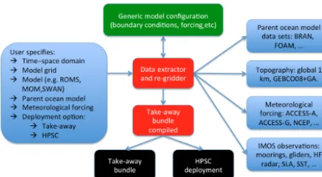
Figure 1.Schematic outlining the steps in WebMARVL. User re-quirements are specified through the WebMARVL interface. The system then selects the grid, the model(s), the parent model(s) for initialisation and boundary conditions, the topography, and meteo-rological forcing. The system subsequently interpolates the inputs to the specified grid requirements. Depending on the deployment option (a) the files are bundled up as a take-away package or (b) de-ployed to a high-performance supercomputer (HPSC).
Setting up models and bringing together the necessary data for initialisation, forcing, and validation is a time-consuming and frequently laborious activity, often taking months to achieve a starting point for scientific investigation. Previous developments have established tools for efficiently configur-ing specific models. For example, Penven et al. (2007) de-scribe a system for configuring a model for the Regional Ocean Model. Real-time applications, including support for defence services and search and rescue, motivated the devel-opment of tools enabling the rapid configuration and deploy-ment of regional ocean forecasts (Rosebrock et al., 2015). Building on this capability, a new infrastructure – called the Web-based Marine Virtual Laboratory (WebMARVL; http: //www.marvl.org.au; http://portal.marvl.org.au) – has been developed. A schematic diagram showing the services and options offered by WebMARVL is presented in Fig. 1. Auto-mated and semi-autoAuto-mated components of the WebMARVL workflow increase functionality and significantly reduce the startup time of any project involving simulation studies of the ocean.
WebMARVL allows a user to quickly and easily configure an ocean general circulation or wave model through a Web-based portal. The user is prompted to select the model, tem-poral extent of the model run, spatial extent, and input data. WebMARVL currently supports three community ocean gen-eral circulation models and two community wave models:
– Regional Ocean Modelling System (ROMS; Shchep-etkin and McWilliams, 2005);
– Modular Ocean Model (MOM; Griffies, 2009);
– Sparse Hydrodynamic Ocean Code (SHOC; Herzfeld, 2009);
– Simulating WAves Nearshore model (SWAN; Booij et al., 1999);
– WaveWatch III (WW-III; Tolman, 2002).
The temporal extent of the model runs is limited to historical periods – not currently permitting forecasts.
Once all aspects of the configuration are selected, a se-ries of services automatically perform the data extraction, re-formatting, and repackaging. WebMARVL produces a “take-away bundle” that contains all of the input fields and forcing fields in the correct format to be immediately used to run the chosen model (e.g. ROMS or MOM). The take-away bundle also includes all of the observations, exploiting capabilities developed under the Australian Integrated Marine Observ-ing System (IMOS; http://www.imos.org.au; Hill et al., 2010; Proctor et al., 2010; Hidas et al., 2016), in the chosen time– space domain. The observations are intended to be used for model assessment and/or data assimilation. The take-away bundle is available to the user via direct download from Web-MARVL. If a user is to manually undertake each step of gath-ering topographic data, ocean input data (from a global ocean model run or reanalysis, for initial conditions and nesting), surface forcing data (from an atmospheric model run or re-analysis), and observational data – and then write a series of scripts to “massage” the data into appropriate formats – the process of setting up a model can take days for an expert and months for a non-expert. By contrast, it takes 5–10 min, de-pending on the computer load, to generate a take-away bun-dle using WebMARVL. The model configuration from the take-away bundle is intended to be a starting point. It is ex-pected that the expert user will refine the model set-up (e.g. mixing schemes, adjustments to topography or coastlines) to improve the model performance for the given application.
The WebMARVL developments are motivated to deliver benefits to the marine community by enabling
– efficient configuration of a range of ocean and wave models;
– efficient model inter-comparisons;
– assessment of the sensitivity studies, comparing model results with different model parameterisations (e.g. mix-ing schemes) and configurations (e.g, oceanic and atmo-spheric forcing);
– efficient configuration of ensemble prediction (in a his-torical sense) – to help quantify uncertainty – using a single model with different input data or using multiple models;
– comprehensive model evaluation through model– observation comparisons;
Figure 2.Screenshots of sample WebMARVL login screens.
– efficient access to and consolidation of observational data for a selected time–space domain.
In this paper, we describe WebMARVL in more detail in Sect. 2, followed by results in Sect. 3, and an example of the data generated by the take-away bundle in Sect. 4. The results presented below typically compare output from man-ually configured models to WebMARVL-configured mod-els. Some test cases also compare WebMARVL-configured models to observations. We seek to demonstrate that the WebMARVL-configured model runs are credible – providing a good foundation for scientific research. We expect that an expert modeller can generate a take-away bundle using Web-MARVL and subsequently refine the model set-up to pro-duce model results of suitable quality to permit high-quality scientific research. Indeed, it is shown in this paper that the automatically configured model configurations produce cred-ible results. The paper concludes with a short discussion and summary in Sect. 5.
2 WebMARVL
The development of WebMARVL was largely funded un-der the Australian National Collaborative Research Infras-tructure Strategy, through the National eResearch Collabo-ration Tools and Research (NeCTAR; http://www.nectar.org. au) programme. NeCTAR is a programme motivated to es-tablish research software infrastructure to promote and sup-port collaborative research outcomes between Australian re-searchers. Consequently, the initial version of WebMARVL is restricted to Australia-based researchers, with user authen-tication provided securely via the Australian Access Feder-ation (AAF; Fig. 2). This means that researchers with lo-gins at Australian universities (e.g. UTAS) and Australian research organisations (e.g. CSIRO) simply use their insti-tutional login name and password to log into WebMARVL.
An incomplete list of the eligible universities is evident in Fig. 2. This aspect of WebMARVL can easily be changed to include international users (e.g. by including AAF Virtual Home, http://vho.aaf.edu.au) with a modest additional devel-opment.
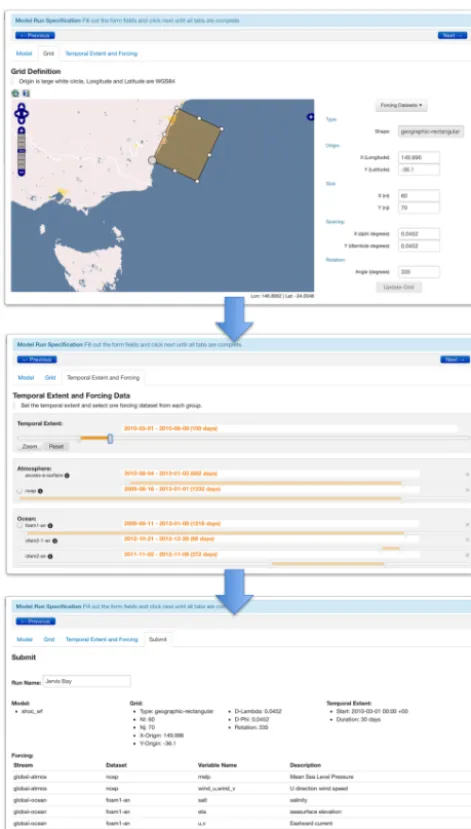
After logging in, a user is prompted to select the model (e.g. ROMS, MOM) from the list of supported models (see Sect. 1) and is prompted to generate a model grid (Fig. 3). The initial version of WebMARVL is restricted to the gen-eration of rectangular grids, so a user effectively needs to specify the corners of the model grid, the angle of rotation, and the grid resolution. This can be done manually – e.g. by typing in the desired reference points – or by a graphical user interface. The user can zoom in and out of the map in the in-terface to carefully define the grid of choice. WebMARVL also offers the option to import files containing one’s own model grid and bathymetry (for ROMS and SHOC only at this stage).
The user is then prompted to define the temporal extent of the model run using a sliding bar (Fig. 3). As the user modi-fies the temporal extent, the choice of input data – including the surface forcing data and ocean data – automatically up-dates. WebMARVL maintains a number of data products that can be used for surface forcing and ocean data. The available atmospheric data sets to be used for surface forcing include
– archived fields from analyses and nowcasts using the Australian Community Climate and Earth System Sim-ulator (ACCESS), Australia’s operational global and re-gional atmospheric prediction systems (ACCESS-G and ACCESS-R; Puri et al., 2010);
– the NCEP/NCAR atmospheric reanalysis (NCEP1; Kalnay et al., 1996).
con-Figure 3.Screenshots of WebMARVL showing the steps of (top to bottom) configuring a grid, setting the temporal extent and selecting input data, and submitting a job.
figuration of WW-III (Tolman, 2002). The available ocean data sets to be used for initial conditions and nesting include – version 3p5 of the Bluelink ReANalysis (BRAN3p5;
Oke et al., 2013);
– archived nowcasts and analyses from the Ocean Mod-elling, Analysis, and Prediction System (OceanMAPS; Brassington et al., 2007), Australia’s operational short-range ocean forecast system;
– the UK Forecasting Ocean Assimilation Model (FOAM; Blockley et al., 2012);
– the Mercator Ocean Global Ocean ReanalYsis and Sim-ulation (GLORYS) (Ferry et al., 2007).
Of these ocean data sets, OceanMAPS and FOAM are archives of nowcasts produced operationally by the Aus-tralian Bureau of Meteorology (BoM) and the UK Met Of-fice; others are from model runs performed under Bluelink – a partnership between CSIRO, the BoM, and the Royal Aus-tralian Navy (Schiller et al., 2009) – or provided by the Mer-cator consortium. As the user adjusts the temporal domain, only the data sets that span the full requested temporal extent are available for selection. Once the user selects the input data, the request is submitted to WebMARVL and a series of scripts are run automatically to perform the following steps:
– data verification – checking that the chosen data sets have the mandatory variables for the chosen model; – data extraction – including the forcing data and
obser-vations;
– reformatting – to put the netcdf files in the format re-quired by the chosen model, including variable and di-mension names, grid constructions, etc.;
– repackaging – to collate all of the required data into a single, easy-to-download package.
Data extraction is achieved through a combination of local files and the Open-source Project for a Network Data Ac-cess Protocol (OPenDAP). Note that the data extraction step, listed above, includes interpolation of fields for some mod-els. For applications of ROMS and MOM, fields are interpo-lated onto the model grids using bilinear interpolation hor-izontally and linear interpolation vertically, using a spheri-cal map projection. For applications of SHOC, SWAN, and WW-III, fields from the original parent grids are supplied to the model. In addition, for applications to SWAN, fields are bilinearly interpolated along the open boundaries to pro-vide boundary forcing. All calculations by WebMARVL are performed on a virtual machine, exploiting readily available open-source software (e.g. GNU compilers, netcdf libraries and operators, Gridgen). Once all WebMARVL tasks are complete, the user can access his or her take-away bundle directly from the Web portal. The user is then free to use and modify the data in the take-away bundles as needed for his or her specific application.
3 Results
Figure 4. Map of Australia, showing the sea level (colour) and geostrophic surface velocities (from http://oceancurrent.imos.org. au), with the approximate locations of each model domain used for testing. Labels, arrows, and boxes are colour-coded for clarity off eastern Australia.
performed under this project during the development of Web-MARVL. This includes one test case using SHOC, one using MOM, two using ROMS, and two using SWAN. Although WebMARVL supports applications with WW-III, a test case for WW-III is not presented in this paper. The results pre-sented here typically compare output from manually config-ured models to WebMARVL-configconfig-ured models. Some test cases also compare WebMARVL-configured models to ob-servations. We seek to demonstrate that the WebMARVL-configured model runs are credible. We expect that an ex-pert modeller can generate a take-away bundle using Web-MARVL and subsequently refine the model set-up to pro-duce model results of suitable quality to permit high-quality scientific research.
3.1 Southern Great Barrier Reef – SHOC
Motivated to better understand what factors affect upwelling and cross-shelf exchange on the Southern Great Barrier Reef (SGBR), particularly near Heron Island, a manually and WebMARVL-configured SHOC run is performed for a do-main over the SGBR (Fig. 4) for the period November 2008 to March 2009. This period spans a series of events when cold water is observed in temperature records obtained from in situ moorings to be uplifted onto the reef, representing strong cross-shelf exchange. Results from BRAN3p5 (Oke et al., 2013), with ∼10 km grid spacing, do not show this same uplift as observed. To determine the extent to which re-analysis represents the dominant processes, a high-resolution regional model is configured to see if it could represent the uplift. The model grid is 2 km in both configurations. The manually configured run is forced at the surface by wind
stress and bulk heat fluxes using fields from ERA-Interim, and the model initial conditions and boundary fields are de-rived from BRAN3p5. The WebMARVL configuration is forced at the surface by wind stress and bulk heat fluxes us-ing fields from ACCESS-R and ocean fields from BRAN3p5. Unlike the BRAN3p5 runs, the regional configuration of SHOC includes tidal forcing at the boundaries. Neither con-figuration includes freshwater fluxes.
Results are shown in Fig. 5, showing initial conditions (panels a–b) and model fields after 18 days of integration (panels c–d), during a strong upwelling/uplifting event. Note that, although the model resolution is the same in the manu-ally configured and the WebMARVL-configured model, the grids are slightly rotated relative to each other. Due to this ro-tation the bottom topography along the two cross-shelf tran-sects are slightly different at the offshore end.
Recall that the goal of these comparisons is to estab-lish the credibility of WebMARVL. To this end, we note that the initial conditions are comparable in both configu-rations (Fig. 5a–b). In part, the differences in initial con-ditions is because the WebMARVL-configured run are ini-tialised 4 days earlier to allow the tides to somewhat equi-librate. But note that WebMARVL does not generate tide boundary conditions. The sub-surface model fields during the upwelling/uplifting events are also very similar (Fig. 5c– d) – both showing sub-22◦ temperatures uplifted onto the reef (around 50 m depth). However, the near-surface temper-atures are quite different, with the WebMARVL-configured run showing warmer surface temperatures, owing to known biases in the fluxes derived from ACCESS-R.
Based on these results, we conclude that the∼10 km reso-lution model lacks sufficient resoreso-lution to represent the uplift of cold water onto the reef over the SGBR. Additionally, the comparisons demonstrate that for this case the WebMARVL-configured model reproduces results that compare well to re-sults from a manually configured model with comparable res-olution and forcing.
3.2 Southeastern Australia – ROMS
Motivated to assess WebMARVL in a region of complex to-pography in the presence of a strong western boundary cur-rent – namely the East Australian Curcur-rent (EAC) – a 1 km resolution configuration of ROMS is applied to a region off Coffs Harbour (∼30◦S; Fig. 4) in the vicinity of the Soli-tary Island Marine Park. This region is of particular inter-est because it is the focus of several national and state pro-grammes (e.g. National Environmental Science Programme, http://www.environment.gov.au/science/nesp) and is the lo-cation of both state and federal marine reserves. The region is also covered by an array of land-based high-frequency (HF) radars – returning high spatial and temporal resolution obser-vations of surface currents.
forc-Figure 5.Comparison of a temperature section off the Southern Great Barrier Reef (Fig. 4) from the SHOC model, using(a, c)a WebMARVL configuration and(b, d)a manual configuration for(a–b)1 December 2008 and(c–d)18 December 2008.
ing from ACCESS-R, and ocean initial conditions and forc-ing from BRAN3p5. The model is run for the period April to July 2012.
When compared to results from BRAN3p5, the WebMARVL-configured ROMS run produced along-shore currents that are more baroclinic (with 50 % stronger alongshore currents) and with more variability in surface temperature (ROMS ranging from 11.2 to 26.7◦C and BRAN3p5 ranging from 18 to 25.5◦C), due to better-resolved processes.
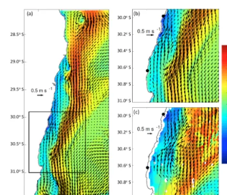
The model results (Fig. 6a) agree reasonably well with ob-servations from different platforms, including satellite sea surface temperature (SST) (with differences of 0.5–0.8◦C) and moorings (with upper-ocean temperature differences of 0.8◦C and correlations of 0.86, and velocity differences of 0.11–0.26 m s−1, with correlations of 0.41–0.45), and with HF radar-derived surface velocities. In particular, the WebMARVL-configured ROMS run shows very detailed sub-mesoscale variability. Figure 6a shows an example of the EAC instabilities at the inshore edge. These frontal vor-tices and eddies are important for driving vertical dynamics and ultimately nutrient supply and biological activity. Both the modelled and observed velocity fields derived from HF radars show such sub-mesoscale eddy structures on the edge of Coffs Harbour (Fig. 6b, c; see also Fig. 3 in Roughan et al., 2015). Although the precise location of the eddy dif-fers, its size and intensity compare qualitatively well. This test case demonstrates that a WebMARVL-configured high-resolution ROMS run can realistically reproduce both the mesoscale and sub-mesoscale variability in a complex region of strong currents. Analysis of the WebMARVL-configured ROMS is ongoing and promises to provide important insights into the cross-shelf processes, upwelling and connectivity, in the Solitary Island Marine Park area off eastern Australia.
Figure 6.Snapshots of(a, b)modelled and(c)observed surface ve-locity and SST for 15 May 2012. Model results are from a 1 km res-olution WebMARVL-configured ROMS run off southeastern Aus-tralia (Fig. 4), and observations are from 6-day composite satellite Advanced Very High Resolution Radiometer (AVHRR) SST and land-based HF radar measurements (the location of the HF radar sites are shown by black dot inb andc). The coastline and 100, 200, 1000, 2000, and 5000 m isobaths are shown in grey. For clar-ity, velocity vectors are only plotted every fifth grid point in(a), every fourth grid point in(b), and every third point for the HF radar data in(c).
3.3 Southwestern Australia – ROMS
Figure 7.Comparisons between observed (HF radar; red) and WebMARVL-configured ROMS (black) surface velocity(a–b)and time series of observed (ADCP; red) and WebMARVL-configured ROMS (black) at 10 m depth at the ADCP location, off the coast of Western Australia. The location of ADCP is denoted by the black dots in(a, b).
model is set up to cover part of the Perth Canyon and Rot-tnest continental shelf, off southwestern Australia (Fig. 4). The model is run for the period July to October 2011. At the time of testing, WebMARVL did not provide fields of evap-oration and precipitation. For this case, however, the users supplemented the WebMARVL take-away bundle with these fields from ERA-Interim. The model is also forced at the boundary with tidal forcing, using eight primary harmonic constituents (specified by the user – not from WebMARVL). Model results are compared to near-surface velocities from HF radar and sub-surface velocities from a moored acoustic Doppler current profiler (ADCP). Results of comparisons be-tween modelled and observed fields are presented in Fig. 7. This includes a comparison of daily averaged modelled and observed near-surface velocities on 13 and 16 July 2011 – when there is a distinct cyclonic eddy present on the shelf edge (Fig. 7a–b). These comparisons show that the model re-alistically reproduces this dominant feature, with good agree-ment in the location, strength, and size of the eddy. A com-parison of time series of the velocity at 10 m depth, measured by a moored ADCP from the IMOS Rottnest Island National Reference Station, is presented in Fig. 7c–d. These compar-isons show very good agreement between the observed and modelled velocities.
The results from this test case demonstrate that, with some additional refinement of the WebMARVL-configured very high resolution ROMS, model results in excellent agreement
with observations can be achieved. Fields from these model runs are being analysed in detail to examine the dynamics of deep water overflows that frequently occur off Western Aus-tralia due to winter cooling (Pattiaratchi et al., 2011). 3.4 Southeastern Australia – MOM
To assess the performance of WebMARVL for setting up a high-resolution configuration of MOM4p1, a 2 km resolution model off southeastern Australia (Fig. 4) is set up. The model has 51 vertical levels and is nested within OceanMAPS and forced at the surface with atmospheric fields from ACCESS-G. The fields presented in Fig. 8 show the initial conditions – representing an interpolation from the∼10 km resolution grid of OceanMAPS to the 2 km resolution grid of the re-gional domain. Also shown in Fig. 8 are the model fields after 16 days of simulation. Evident in Fig. 8 is that the high-resolution model adds significant detail to the fields – with the generation of fine-scale filaments and sub-mesoscale ed-dies. Although this demonstration does not assess the skill of the high-resolution configuration, it does demonstrate that the WebMARVL can be used as a starting point for a regional configuration of MOM.
3.5 Southeastern Australia – SWAN
con-Figure 8.Snapshots of(a–b)sea surface temperature and(c–d) sur-face salinity for the(a, c)initial conditions, interpolated from a 0.1◦ resolution model (OceanMAPS), and(b, d)the model fields after 16 days of evolution by a 2 km resolution model.
sidered. One domain is off Sydney (∼33.75◦S), and the second is off Coffs Harbour (∼30.3◦S). The approximate locations of the model domains are shown in Fig. 4. The Sydney test case is motivated to assess the performance of the WebMARVL-configured SWAN model near the coast, in shallow water. The Coffs Harbour test case is motivated to assess the performance farther offshore, in deeper water.
The Sydney configuration has 50 m horizontal resolution, spanning a ∼13×22 km rectangular grid offshore of the northern beaches of Sydney. Two WebMARVL configura-tions are tested for this domain: one forced by 12 km reso-lution ACCESS-R winds (hereafter MARVL SWAN: BoM) and one forced with 20 km resolution NCEP winds (hereafter MARVL SWAN: NCEP). These runs were compared to a manually configured SWAN model by Cardno (2011), here-after Manual SWAN: OEH (NSW Office of Environment and Heritage). MARVL SWAN: BoM is forced with winds from ACCESS-R and nested inside AUSWAVE (Durrant et al., 2013). Manual SWAN: OEH is forced with winds from the NCEP/NCAR atmospheric reanalysis and nested inside a se-ries of four coarser grids (a SWAN “transfer” grid and state, national and global configurations of WW-III). Established in 2011, the Manual SWAN: OEH model is carefully con-figured and tuned for the NSW coastline (including Sydney and Coffs Harbour regions) including adjustments to forc-ing NCEP/NCAR wind speeds within 100 km of the NSW coast. Time series of observed significant wave height ap-proximately 1 km offshore in 21 m of water are compared with Manual SWAN: OEH model time series at the same lo-cation and MARVL SWAN: BoM from the nearest available
Figure 9.Time series of modelled (colour) and observed (black) significant wave height off Sydney (∼1 km offshore, in 21 m of wa-ter), for two different model configurations –(a)MARVL SWAN: BoM and(b)Manual SWAN: OEH.
wet cell (1.4 km seaward of the wave buoy) in Fig. 9. Al-though the WebMARVL-configured SWAN run produces re-sults that are qualitatively consistent with observations (i.e. generally following the “shape” of wave episodes measured by the wave buoy), the automatically configured model sig-nificantly under-predicts peak wave heights for individual storm events in shallow water. Similar performance was ob-served with the MARVL SWAN: NCEP model (not shown). The key reason for this difference is errors in topography and the position of the model coastline, which is gener-ally located several kilometres offshore of the true coastline (i.e. 0 m contour). WebMARVL extracts topography from the Australian Bathymetry and Topography Grid (Whiteway, 2009) produced by Geoscience Australia, which has reso-lution of 9 arcsec (∼280×280 m) and is too coarse to be useful for very high resolution applications in shallow water, close to the coastline in this region.
Figure 10.Time series of modelled (colour) and observed (black) significant wave height off Coffs Harbour (∼12 km offshore, in 72 m of water), for three different model configurations – Man-ual SWAN: OEH (red,a); MARVL SWAN: NCEP (blue,b); and MARVL SWAN: BoM (green,c).
The test cases presented here lead to the conclusion that the WebMARVL-configured wave model is suitable for op-erational climate science modellers (i.e. relatively deep water applications, say>50 m depth) but is not recommended for engineering design and/or shallow-water applications. The primary reasons for this conclusion are limitations in the to-pography and less reliable performance under extreme storm wave conditions (infrequent events). The topography that currently underpins WebMARVL is too coarse (∼280 m res-olution) for very high resolution (50–100 m grids) near the coast – where the location of the coastline is often poorly rep-resented in the automatically configured models. However, in order to overcome this limitation, WebMARVL also enables the user to upload his or her own topography if necessary.
4 Take-away bundles
To give the reader an idea of the data that are typically pro-vided in the take-away bundles produced by WebMARVL, we provide some technical details of one of the examples above. For this demonstration, we report on the take-away bundle associated with the MOM example (Example 3.4). Files generated for MOM include
– grid_spec.nc: a netcdf data file containing information about the model grid and topography;
– mom.nc: a netcdf data file containing four-dimensional fields of temperature, salinity, velocity, and sea level that are used to force the model (i.e. boundary forcing and optionally sponge forcing) and three-dimensional (horizontal dimensions and time) fields of wind stress, heat flux components, and freshwater flux components (excluding river forcing);
– ocean_temp_salt.res.nc: a netcdf data file containing three-dimensional (horizontal and vertical dimensions) fields of temperature, salinity, velocity, and sea level that are used to initialise the model;
– data_table: a text file containing logical flags, variable names, and parameters to define the surface forcing for the model and to define what output the model will gen-erate;
– ocean_solo.res: a text file containing information about the model start date, run length, and calendar type. Note that the mom.nc file, listed above, contains many fields that are commonly stored in separate files for MOM runs. These includes the sponge files, the restore files, and the force files. In addition to these files, the model requires a series of name lists to be defined to specify the options defining the model’s numerics, forcing, etc. These name lists are gener-ally defined in a run script that is prepared by the user.
5 Discussion and summary
A new Web-based tool, called WebMARVL, has been de-veloped to increase the efficiency of configuring a regional ocean model. The development of WebMARVL was under-taken by CSIRO and UTAS, and tested by a cross section of the Australian coastal ocean modelling community. Tests of the system were performed by researchers from seven dif-ferent research organisations, using five difdif-ferent community models (i.e. SHOC, ROMS, MOM, SWAN, and WW-III). The time taken to configure any of the chosen regional mod-els using WebMARVL is just a few minutes. This contrasts to the traditional manual approach, taking days to months – depending on the proficiency of the modeller.
starting point for scientific research. WebMARVL is freely available to researchers associated with Australian research organisations, and there are plans to make it available glob-ally. It is anticipated that, by delivering improved efficiency to the coastal ocean modelling community, WebMARVL will become a valuable research tool – helping experienced and student modellers to more quickly get to the heart of a scien-tific study.
6 Code availability
MARVL software (version 2.1) is open-source code that is available under an MIT license. However, software for all of the underpinning models are available under open-source licensing. ROMS software (version 3.4, revision 633) is available from http://www.myroms.org. MOM soft-ware (version 4p1) is available from http://mom-ocean. org/web. SHOC software (version 1.1, revision 4718) is available from http://www.emg.cmar.csiro.au. SWAN soft-ware (version 40.91AB) is available from http://swanmodel. sourceforge.net. Gridgen software is available from https: //github.com/sakov/gridgen-c. Netcdf operators software is available from http://nco.sourceforge.net. GNU compilers are available from http://gcc.gnu.org.
Acknowledgements. Funding for this research was provided by National eResearch Collaboration Tools and Research (NeCTAR; sub-contract VL206), UTAS, and CSIRO. Data were sourced from the Integrated Marine Observing System (IMOS) – IMOS is supported by the Australian Government through the National Col-laborative Research Infrastructure Strategy and the Super Science Initiative. Wave buoy observations were collected and provided by Manly Hydraulics Laboratory (MHL). Wave buoy observations and the manual configured SWAN models are owned by the NSW Office of Environment and Heritage (OEH). The authors also acknowledge J. Luick and R. Morrison, who contributed to the MARVL project as testers.
Edited by: R. Marsh
Reviewed by: two anonymous referees
References
Blockley, E. W., Martin, M. J., and Hyder, P.: Validation of FOAM near-surface ocean current forecasts using Lagrangian drift-ing buoys, Ocean Sci., 8, 551–565, doi:10.5194/os-8-551-2012, 2012.
Booij, N., Ris, R. C., and Holthuijsen, L. H.: A third-generation wave model for coastal regions: 1. model descrip-tion and validadescrip-tion, J. Geophys. Res.-Oceans, 104, 7649–7666, doi:10.1029/98JC02622, 1999.
Brassington, G. B., Pugh, T. F., Spillman, C., Schulz, E., Beggs, H., Schiller, A., and Oke, P. R.: Bluelink development of operational oceanography and servicing in Australia, J. Res. Pract. Inf. Tech., 39, 151–164, 2007.
Cardno, A.: NSW coastal waves: Numerical modelling. final report, in: Final Report, Office of Enviornment and Heritage (NSW), September, 122 pp., 2011.
Durrant, T. H., Greenslade, D. J., and Simmonds, I.: The effect of statistical wind corrections on global wave forecasts, Ocean Model., 70, 116–131, 2013.
Ferry, N., Remy, E., Brasseur, P., and Maes, C.: The Mercator global ocean operational analysis system: Assessment and val-idation of an 11-year reanalysis, J. Marine Syst., 65, 540–560, doi:10.1016/j.jmarsys.2005.08.004, 2007.
Griffies, S. M.: Elements of MOM4p1, GFDL Ocean Group Tech-nical Report 6, Tech. rep., NOAA/Geophysical Fluid Dynamics Laboratory, 2009.
Herzfeld, M.: Improving stability of regional numerical ocean mod-els, Ocean Dynam., 59, 21–46, doi:10.1007/s10236-008-0158-1, 2009.
Hidas, M. G., Proctor, R., Atkins, N., Atkinson, J., Besnard, L., Blain, P., Bohm, P., Burgess, J., Fruehauf, D., Galibert, G., Hoen-ner, X., Hope, J., Jones, C., Mancini, S., Pasquer, B., Nahodil, D., Reid, K., and Tattersall, K.: Infrastructure and workflows for aus-tralia’s integrated marine observing system, Earth Sci. Inform., doi:10.1007/s12145-016-0266-2, online first, 2016.
Hill, K., Moltmann, T., Proctor, R., and Allen, S.: The Australian integrated marine observing system: Delivering data streams to address national and international research priorities, Mar. Tech-nol. Soc. J., 44, 65–72, 2010.
Kalnay, E., Kanamitsu, M., Kistler, R., Collins, W., Deaven, D., Gandin, L., Iredell, M., Saha, S., White, G., Woollen, J., Zhu, J., Chelliah, M., Ebisuzaki, W., Higgins, W., Janowiak, J., Mo, K., Ropelewski, C., Wang, J., Leetmaa, A., Reynolds, R. W., Jenne, R., and Joseph, D.: The NCEP/NCAR 40-year reanalysis project, B. Am. Meteorol. Soc., 77, 437–471, 1996.
Oke, P. R., Sakov, P., Cahill, M. L., Dunn, J. R., Fiedler, R., Griffin, D. A., Mansbridge, J. V., Ridgway, K. R., and Schiller, A.: Towards a dynamically balanced eddy-resolving ocean reanalysis: BRAN3, Ocean Model., 67, 52–70, doi:10.1016/j.ocemod.2013.03.008, 2013.
Pattiaratchi, C., Hollings, B., Woo, M., and Welhena, T.: Dense shelf water formation along the south-west australian inner shelf, Geophys. Res. Lett., 38, L10609, doi:10.1029/2011GL046816, 2011.
Penven, P., Marchesiello, P., Debreu, L., and Lefevre, J.: Software tools for pre- and post-processing of oceanic regional simula-tions, Environ. Model. Softw., 23, 660–662, 2007.
Proctor, R., Roberts, K., and Ward, B. J.: A data delivery system for IMOS, the Australian Integrated Marine Observing System, Adv. Geosci., 28, 11–16, doi:10.5194/adgeo-28-11-2010, 2010. Puri, K., Xiao, Y., Sun, X., Lee, J., Engel, C., Steinle, P., Le, T.,
Bermous, I., Logan, L., Bowen, R., Sun, Z., Naughton, M., Roff, G., Dietachmayer, G., Sulaiman, A., Dix, M., Rikus, L., Zhu, H., Barras, V., Sims, H., Tingwell, C., Harris, B., Glowacki, T., Chattopadhyay, M., Deschamps, L., and Le Marshall J.: Prelim-inary results from numerical weather prediction implementation of ACCESS, CAWCR Res. Lett., 5, 15–22, 2010.
Roughan, M., Schaeffer, A., and Suthers, I. M.: Chapter 6 – sus-tained ocean observing along the coast of southeastern aus-tralia: Nsw-imos 2007–2014, in: Weisberg YLKH (ed) Coastal Ocean Observing Systems, Academic Press, Boston, 76–98, doi:10.1016/B978-0-12-802022-7.00006-7, 2015.
Schiller, A., Meyers, G., and Smith, N.: Taming australia’s last fron-tier, Am. Meteorol. Soc. Bull., 90, 436–440, 2009.
Shchepetkin, A. and McWilliams, J. C.: The regional oceanic mod-eling system (roms): a split-explicit, free-surface, topography-following-coordinate oceanic model, Ocean Model., 9, 347–404, doi:10.1016/j.ocemod.2004.08.002, 2005.
Tolman, H. L.: User manual and system documenta-tion of WAVEWATCH-III version 2.22, Vol. 133, NOAA/NWS/NCEP/MMAB Technical Note 222, 2002. Whiteway, T. G.: Australian bathymetry and topography grid,