www.geosci-model-dev.net/9/1/2016/ doi:10.5194/gmd-9-1-2016
© Author(s) 2016. CC Attribution 3.0 License.
Integration of nitrogen dynamics into the Noah-MP land surface
model v1.1 for climate and environmental predictions
X. Cai1,a, Z.-L. Yang1, J. B. Fisher2,3, X. Zhang4, M. Barlage5, and F. Chen5
1Department of Geological Sciences, The John A. and Katherine G. Jackson School of Geosciences, The University of Texas at Austin, Austin, Texas, USA
2Jet Propulsion Laboratory, California Institute of Technology, Pasadena, California, USA
3Joint Institute for Regional Earth System Science and Engineering (JIFRESSE), University of California at Los Angeles, Los Angeles, California, USA
4Joint Global Change Research Institute, Pacific Northwest National Laboratory and University of Maryland, College Park, Maryland, USA
5Research Applications Laboratory, National Center for Atmospheric Research, Boulder, Colorado, USA anow at: Department of Civil and Environmental Engineering, Princeton University, Princeton, New Jersey, USA Correspondence to: Z.-L. Yang ([email protected])
Received: 11 April 2015 – Published in Geosci. Model Dev. Discuss.: 27 May 2015 Revised: 12 October 2015 – Accepted: 11 December 2015 – Published: 15 January 2016
Abstract. Climate and terrestrial biosphere models consider nitrogen an important factor in limiting plant carbon uptake, while operational environmental models view nitrogen as the leading pollutant causing eutrophication in water bod-ies. The community Noah land surface model with multi-parameterization options (Noah-MP) is unique in that it is the next-generation land surface model for the Weather Re-search and Forecasting meteorological model and for the op-erational weather/climate models in the National Centers for Environmental Prediction. In this study, we add a capabil-ity to Noah-MP to simulate nitrogen dynamics by coupling the Fixation and Uptake of Nitrogen (FUN) plant model and the Soil and Water Assessment Tool (SWAT) soil nitro-gen dynamics. This model development incorporates FUN’s state-of-the-art concept of carbon cost theory and SWAT’s strength in representing the impacts of agricultural manage-ment on the nitrogen cycle. Parameterizations for direct root and mycorrhizal-associated nitrogen uptake, leaf retranslo-cation, and symbiotic biological nitrogen fixation are em-ployed from FUN, while parameterizations for nitrogen min-eralization, nitrification, immobilization, volatilization, at-mospheric deposition, and leaching are based on SWAT. The coupled model is then evaluated at the Kellogg Biological Station – a Long Term Ecological Research site within the US Corn Belt. Results show that the model performs well
in capturing the major nitrogen state/flux variables (e.g., soil nitrate and nitrate leaching). Furthermore, the addition of ni-trogen dynamics improves the modeling of net primary pro-ductivity and evapotranspiration. The model improvement is expected to advance the capability of Noah-MP to simulta-neously predict weather and water quality in fully coupled Earth system models.
1 Introduction
hypoxia extent (Donner and Scavia, 2007): higher tempera-tures may extend the thermal stratification period and deepen the thermocline, thereby resulting in the upwelling of nutri-ents from sediment and increasing the concentration of nu-trients in the bottom layer of water in lakes (Komatsu et al., 2007). Further, higher precipitation produces more runoff, and very likely more nutrients are delivered to the ocean as well (Donner and Scavia, 2007).
Nitrogen (N) is recognized as the leading nutrient caus-ing eutrophication. Without human interference, N cyclcaus-ing is relatively slow, as most ecosystems are efficient at retain-ing this in-demand nutrient. N enters soil regularly either through atmospheric wet and dry deposition or through at-mospheric N2fixation by microorganisms (occurring mostly in legume plants). N taken up by plants is confined to rel-atively slow processes (e.g., growth, decay, and mineraliza-tion); in some regions or during the growing season, N may also limit plant growth, which reduces carbon sequestration over land (Fisher et al., 2012). In addition, N cycling pro-duces nitrous oxide (N2O), which is considered one of the important greenhouse gases responsible for climate warm-ing. These facts make the N cycle important for studying the response of the climate to the elevated greenhouse gas con-centrations. With human tillage of soils, mineralization and nitrification of N are amplified, which results in the reduc-tion of N storage in soil (Knops and Tilman, 2000; Scanlon et al., 2008). In addition, a large amount of N fertilizer is applied in specific areas within a short period of time; as a result, a massive excess of N is leached to the aquatic sys-tems through discharge and erosion, which contributes to the eutrophication in aquatic systems.
Many of these N processes have been included in land sur-face, hydrologic, and water quality models developed partic-ularly for environmental, climate, and agricultural applica-tions (Bonan and Levis, 2010; Dickinson et al., 2002; Fisher et al., 2010; Kronvang et al., 2009; Schoumans et al., 2009; Thornton et al., 2007; Wang et al., 2007; Yang et al., 2009). These developments are still in their infancy, and large-scale climate models lack N leaching parameterizations that are comparable to those used in water quality models. Thus, large-scale models are not feasible for inherently fine-scale applications such as agricultural fertilization management and water quality prediction. Therefore, the present study improves these weaknesses by incorporating the strength of agriculture-based models into large-scale land surface mod-els (LSMs).
The community Noah LSM with multi-parameterization options (Noah-MP) (Niu et al., 2011; Yang et al., 2011) is used as an exemplar of LSMs because it is the next-generation LSM for the Weather Research and Forecast-ing (WRF) meteorological model (Rasmussen et al., 2014) and for the operational weather and climate models in the NOAA/National Centers for Environmental Prediction. Be-cause Noah-MP has an interactive vegetation canopy option – which predicts the leaf area index (LAI) as a function of
light, temperature, and soil moisture – it is logical to aug-ment this scheme with N limitation and realistic plant N up-take and fixation. The state-of-the-art vegetation N model is the Fixation and Uptake of Nitrogen (FUN) model of Fisher et al. (2010), which is embedded into the Joint UK Land Environment Simulator (JULES) (D. B. Clark et al., 2011) and the Community Land Model (CLM) (Shi et al., 2016). Modeling the impacts of agricultural management (e.g., fer-tilizer use) on N leaching is the strength of the Soil and Water Assessment Tool (SWAT) (Neitsch et al., 2011). Therefore, this study incorporates into Noah-MP both FUN’s strength in plant N uptake and SWAT’s strength in soil N cycling and agricultural management.
Our objective is to develop and utilize a land surface mod-eling framework for simultaneous climate (carbon) and en-vironmental (water quality) predictions. We first describe the nitrogen dynamic model which combines equations used in FUN and SWAT. We then focus on evaluating the new inte-grated model at a cropland site, because fertilizer application on croplands globally contributes approximately half of the total N input to soil, with the other half coming from natu-ral processes (i.e., atmospheric deposition and biological N fixation) (Fowler et al., 2013; Gruber and Galloway, 2008). Furthermore, cropland is a major source of N loading in wa-ter bodies. We evaluate the new model against observed soil moisture content, concentration of soil nitrate, concentration of nitrate leaching from soil bottom, and annual net primary productivity (NPP). We then analyze the impacts of the addi-tion of N dynamics on the carbon and water cycles. To guide the use of this model on regional scales, we also analyze the impacts from different fertilizer application scenarios. Fi-nally, we discuss other model behaviors, i.e., N uptake from different pathways and the major soil nitrate fluxes.
2 Models, data, and methods 2.1 Noah-MP
The Noah-MP model was augmented from the original Noah LSM with improved physics and multi-parameterization op-tions (Niu et al., 2011; Yang et al., 2011), based on a state-of-the-art multiple-hypothesis framework (M. P. Clark et al., 2011). Noah-MP provides users with multiple options for parameterization in leaf dynamics, canopy stomatal resis-tance, soil moisture factor for stomatal resisresis-tance, and runoff and groundwater. Until this work, Noah-MP did not include any N dynamics. The only N-related parameterization is in the calculation of the maximum rate of carboxylation (Vmax, Eq. 1) – an important factor in estimating the total carbon assimilation (or photosynthesis) rate (Niu et al., 2011):
Vmax=Vmax25a
Tv−25 10
vmaxf (N )f (Tv)β, (1)
pa-rameter,f (Tv)is a function that mimics the thermal break-down of metabolic processes,f (N )is a foliage nitrogen fac-tor (f (N )≤1), andβis the soil moisture controlling factor. Since there were no N dynamics in the model, f (N ) was set as a constant 0.67, which translates to a constant 33 % of
Vmaxdown-regulation due to N stress. This factor was origi-nally used in Running and Coughlan (1988) and adapted into LSMs by Bonan (1991).
Our modifications to the original Noah-MP mainly con-cern the sub-models dealing with dynamic leaf and subsur-face runoff. The dynamic leaf option is turned on to pro-vide NPP and biomass to the newly coupled N dynamic sub-model. In the original Noah-MP model, subsurface runoff from each soil layer was not an explicit output, but it is now a new output in the updated model. However, N concentrations are different among soil layers, which affects the amount of N removed from each soil layer by subsurface runoff. There-fore, in conjunction with the runoff scheme options 1 (TOP-MODEL with groundwater) and 2 (TOP(TOP-MODEL with an equilibrium water table), the lumped subsurface runoff for all four layers is first calculated, and then the water is removed from each soil layer weighted by hydraulic conductivity and soil layer thickness.
2.2 Nitrogen dynamics
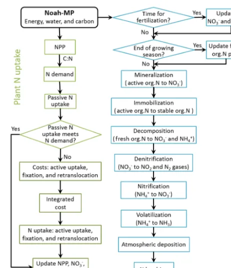
In Noah-MP, the soil N model structure is the same as in SWAT, which includes five N pools consisting of two inor-ganic forms (NH+4 and NO−3)and three organic forms (ac-tive, stable, and fresh pools). The N processes employed from SWAT are mineralization, decomposition, immobilization, nitrification, denitrification, and atmospheric deposition. The N processes employed from FUN are uptake and symbiotic biological N fixation, which can be further divided into active and passive soil N uptake, leaf N retranslocation, and sym-biotic biological N fixation. Figure 1 shows the flow chart of the nitrogen dynamic model. In this section, we describe the core equations. The full description for plant N uptake and soil N dynamics is available in Fisher et al. (2010) and Neitsch et al. (2011), respectively. Table 1 shows the model input variables and parameters. Most of these parameters use the values recommended by Fisher et al. (2010) and Neitsch et al. (2011), while some of them are adjusted to best repre-sent the site condition and hence match site observation. The important adjusted parameters include the γsw,thr (threshold value of soil water factor for denitrification to occur), βmin (rate coefficient for mineralization of the humic organic ni-trogen), and βrsd (rate coefficient for mineralization of the fresh organic nitrogen in residue).
2.2.1 Nitrogen uptake and fixation
Plant N uptake and fixation follow the framework of Fisher et al. (2010), which determines N acquired by plants through Eq. (3), advection (passive uptake); Eq. (4), symbiotic
bi-Figure 1. Flow chart of the nitrogen dynamic model. org.N: organic nitrogen.
ological N fixation; Eq. (5) active uptake; and Eq. (6), re-translocation (resorption).
Noah-MP calculates the NPP or its available carbon,
CNPP (kg C m−2), following FUN. To maintain the pre-scribed carbon-to-nitrogen (C : N) ratio (rC:N), the N de-mand,Ndemand(kg N m−2), is calculated:
Ndemand= CNPP rC:N
, (2)
where rC:N is the C : N ratio for the whole plant, which is computed for each component (leaf, root, and wood) of the plant proportionally to the biomass. C : N ratios for each component of the plant for each vegetation type are from Oleson et al. (2013).
Because no extra energetic cost is needed, passive uptake,
Npassive(kg N m−2), is the first and preferred source of N that a plant depletes:
Npassive=Nsoil ET
sd
, (3)
whereNsoil is the available soil N for the given soil layer (kg N m−2),ET is transpiration rate (m s−1), and sd is the soil water depth (m). This pathway is typically a minor con-tributor except under very high soil N conditions.
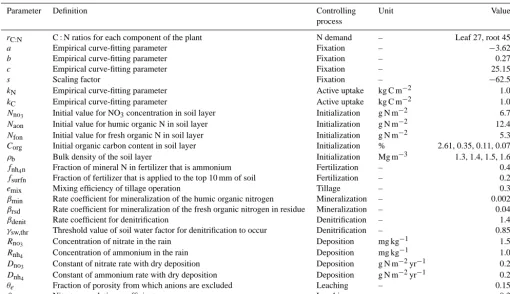
Table 1. Model input variables and parameters.
Parameter Definition Controlling Unit Value
process
rC:N C : N ratios for each component of the plant N demand – Leaf 27, root 45
a Empirical curve-fitting parameter Fixation – −3.62
b Empirical curve-fitting parameter Fixation – 0.27
c Empirical curve-fitting parameter Fixation – 25.15
s Scaling factor Fixation – −62.5
kN Empirical curve-fitting parameter Active uptake kg C m−2 1.0
kC Empirical curve-fitting parameter Active uptake kg C m−2 1.0
Nno3 Initial value for NO3concentration in soil layer Initialization g N m
−2 6.7
Naon Initial value for humic organic N in soil layer Initialization g N m−2 12.4
Nfon Initial value for fresh organic N in soil layer Initialization g N m−2 5.3 Corg Initial organic carbon content in soil layer Initialization % 2.61, 0.35, 0.11, 0.07
ρb Bulk density of the soil layer Initialization Mg m−3 1.3, 1.4, 1.5, 1.6 fnh4n Fraction of mineral N in fertilizer that is ammonium Fertilization – 0.4
fsurfn Fraction of fertilizer that is applied to the top 10 mm of soil Fertilization – 0.2
emix Mixing efficiency of tillage operation Tillage – 0.3
βmin Rate coefficient for mineralization of the humic organic nitrogen Mineralization – 0.002 βrsd Rate coefficient for mineralization of the fresh organic nitrogen in residue Mineralization – 0.04
βdenit Rate coefficient for denitrification Denitrification – 1.4
γsw,thr Threshold value of soil water factor for denitrification to occur Denitrification – 0.85
Rno3 Concentration of nitrate in the rain Deposition mg kg
−1 1.5
Rnh
4 Concentration of ammonium in the rain Deposition mg kg
−1 1.0
Dno3 Constant of nitrate rate with dry deposition Deposition g N m
−2yr−1 0.2
Dnh4 Constant of ammonium rate with dry deposition Deposition g N m−2yr−1 0.2
θe Fraction of porosity from which anions are excluded Leaching – 0.15
βno3 Nitrate percolation coefficient Leaching – 0.3
Note: some parameters are not described in the paper. The values forCorgandρbare for the four soil layers.
(Nfix, kg N m−2), all of which are associated with energetic cost and hence require C expenditure (C cost). The C costs of fixation (Costfix, kg C kg N−1), active uptake (Costactive, kg C kg N−1), and resorption (Costresorb, kg C kg N−1) are calculated as follows:
Costfix=s
expa+b·Tsoil·(1−0.5·Tsoil/c)
−2 , (4) Costactive=
kN Nsoil
kC Croot
, (5)
Costresorb= kR Nleaf
. (6)
where a, b, and c (−3.62, 0.27 and 25.15, respectively) are empirical curve-fitting parameters (dimensionless) from Houlton et al. (2008); s is a scaling factor (= −62.5; use kg C kg N−1◦C for unit consistency);Tsoilis soil temperature (◦C);kN andkC are both 1 kg C m−2; kR is 0.01 kg C m−2; Croot is total root biomass (kg C m−2); and Nleaf is the amount of N in the leaf (kg N m−2). Active uptake is typ-ically a dominant form of N uptake in natural ecosystems, consuming large quantities of NPP (that would otherwise go to growth or other allocations) in exchange for N.
Similar to parallel circuits, each carbon cost is treated as a resistor, and the integrated cost (Costacq, kg C kg N−1)is calculated (Brzostek et al., 2014):
1 Costacq
= 1
Costfix
+ 1
Costresorb +
n
X
i=1 1 Costactive,ly
, (7)
where Costactive,ly is the C cost for active N uptake of soil layer ly andnis the total number of soil layers.
Using Ohm’s law, N acquired from C expenditure (Nacq, kg N m−2)is analogous to current and thus is calculated as follows:
Nacq= Cacq Costacq
. (8)
Therefore, plant N uptake and fixation are computed and are updated for each N pool. In addition, the effect of N limitation on CO2sequestration is represented in the model through the theory of C cost economics.
2.2.2 Mineralization, decomposition, and immobilization
Immobilization is incorporated into mineralization calcu-lation (net mineralization). Mineralization and decomposi-tion, which are only allowed to occur when soil tempera-ture is above 0◦C, are constrained by water availability and temperature. The nutrient-cycling temperature factor for soil layer ly,γtmp,ly, is calculated as follows:
γtmp,ly= (9)
0.9· Tsoil,ly
Tsoil,ly+exp9.93−0.312·Tsoil,ly +0.1,
whereTsoil,lyis the temperature of soil layer ly (◦C). The nutrient-cycling water factor for soil layer ly,γsw,ly, is calculated as follows:
γsw,ly= θly θs,ly
, (10)
whereθlyis the water content of soil layer ly (mm H2O) and θs,ly is the water content of soil layer ly at field capacity (mm H2O).
The mineralized N from the humus active organic N pool,
Nmina,ly(kg N m−2), is calculated as follows: Nmina,ly=βmina,ly γtmp,ly·γsw,ly
1/2
·Naon,ly, (11)
whereβmina is the rate coefficient for mineralization of the humus active organic nutrients andNaon,lyis the amount of N in the active organic pool (kg N m−2).
The mineralized N from the residue fresh organic N pool,
Nminf,ly(kg N m−2), is calculated as follows:
Nminf,ly=0.8·δntr,ly·Nfon,ly, (12) whereδntr,lyis the residue decay rate constant, andNfon,lyis the amount of N in the fresh organic pool (kg N m−2).
The decomposed N from the residue fresh organic N pool,
Ndec,ly(kg N m−2), is calculated as follows:
Ndec,ly=0.2·δntr,ly·Nfon,ly. (13)
2.2.3 Nitrification and ammonia volatilization
Using a first-order kinetic rate equation, the total amount of ammonium lost to nitrification and volatilization in layer ly,
Nnit|vol,ly(kg N m−2), is calculated as follows:
Nnit|vol,ly=NH4,ly· [1−exp(−ηnit,ly−ηvol,ly)], (14) where NH4,ly is the amount of ammonium in layer ly (kg N m−2), ηnit,ly is the nitrification regulator, and ηvol,ly is the volatilization regulator. The calculation of ηnit,lyand ηvol,lyis described in Neitsch et al. (2011).
Nnit|vol,lyis then partitioned to nitrification and volatiliza-tion. The amounts of N converted from NH+4 and NO−3 of the ammonium pool via nitrification and volatilization are then
calculated:
Nnit,ly=
frnit,ly frnit,ly+frvol,ly
·Nnit|vol,ly, (15)
Nvol,ly=
frvol,ly frnit,ly+frvol,ly
·Nnit|vol,ly, (16)
where frnit,lyand frnit,lyare the estimated fractions of N lost through nitrification and volatilization, respectively. They are calculated from the individual regulator in Eq. (14) as fol-lows:
frnit,ly=1−exp[−ηnit,ly], (17)
frvol,ly=1−exp[−ηvol,ly]. (18)
2.2.4 Denitrification
Denitrification is the process of bacteria removing N from soil (converting NO−3 to N2 or N2O gases). Denitrification rate,Ndenit,ly(kg N m−2), is calculated as follows:
Ndenit,ly=NO3,ly· [1−exp(−βdenit·γtmp,ly ·orgCly)] ifγsw,ly≥γsw,thr Ndenit,ly=0 ifγsw,ly≥γsw,thr
, (19)
where orgCly is the amount of organic C in the layer (%), βdenitis the rate coefficient for denitrification, and γsw,thr is the threshold value ofγsw,lyfor denitrification to occur. 2.2.5 Atmospheric deposition
While the mechanism of atmospheric deposition is not fully understood, the uncertainty is parameterized into the concen-tration of nitrate/ammonium in the rain for wet deposition, and the nitrate/ammonium deposition rate for dry deposition. The amounts of nitrate and ammonium added to the soil through wet deposition, NO3,wet (kg N m−2) and NH4,wet (kg N m−2), are calculated as follows:
NO3,wet=0.01·RNO3·P , (20) NH4,wet=0.01·RNH4·P , (21) where RNO3 is the concentration of nitrate in the rain (mg N L−1),RNH4 is the concentration of ammonium in the rain (mg N L−1), andP is the amount of precipitation. The values forRNO3 andRNH4 used in this study are listed in Table 1.
2.2.6 Fertilizer application
2.2.7 Leaching
N leaching from land to water bodies is a consequence of soil weathering and erosion processes. In particular, organic N attached to soil particles is transported to surface water through soil erosion. Therefore, the modified universal soil loss equation (USLE) (Williams, 1995) is used to determine soil erosion. The details of the calculation are described in Neitsch et al. (2011).
N in nitrate form can be transported with surface runoff, lateral runoff, or percolation, which is calculated as follows: NO3,surf=βNO3·concNO3,mobile·Qsurf, (22)
NO3,lat,ly=βNO3
·concNO3,mobile·Qlat,ly for top layer NO3,lat,ly=
concNO3,mobile·Qlat,ly for lower layers
, (23)
NO3,perc=concNO3,mobile·wperc,ly, (24) where NO3,surf, NO3,lat,ly, and NO3,percare the soil nitrates removed in surface runoff, in subsurface flow, and by per-colation, respectively (kg N m−2);β
NO3 is the nitrate perco-lation coefficient; concNO3,mobile is the concentration of ni-trate in the mobile water in the layer (kg N mm H2O−1), and wperc,ly is the amount of water percolating to the underlying soil layer (mm H2O),Qsurf is the generated surface runoff (mm H2O), andQlat,lyis the water discharged from the layer by lateral flow (mm H2O).
2.3 Description of evaluation data and model configuration
At the regional scale, N-related measurements are very lim-ited. Even at site level, measurements are limited with respect to plant and carbon dynamics. The Kellogg Biological Sta-tion (KBS) – a Long Term Ecological Research (LTER) site – is unique in its long-term continuous measurements of N related variables (soil nitrate, N leaching, mineralization, ni-trification, and fertilizer application) in an agricultural setting with multiple crop and soil controls. Even within the LTER Network, we cannot find a second site that conducts this in-tegrated suite of measurements. Therefore, the new model is evaluated at this site.
KBS is located in Hickory Corners, Michigan, USA, within the northeastern portion of the US Corn Belt (42.40◦N, 85.40◦W, elevation 288 m). Mean annual temper-ature is 10.1◦C, and mean annual precipitation is 1005 mm,
with about half falling as snow. This study uses two treat-ments from this site: T1 cropland with conventional tillage and T2 cropland without tillage. Both treatments are rainfed and are planted with the same crops: corn, soybean, and win-ter wheat in rotation.
This site features multiple N-related measurements. Soil inorganic N concentration, which is sampled from the surface to 25 cm soil depth, is available from 1989 to 2012. Concen-tration of inorganic N leaching at bedrock, which is sampled
at 1.2 m of soil depth, is available from 1995 to 2013. These two measurements are used to evaluate model-simulated con-centrations of soil nitrate for the top 25 cm and nitrate leach-ing from the soil bottom. Soil N mineralization, which mea-sures the net mineralization potential and is available from 1989 to 2012, is compared with the modeled mineralization rate qualitatively.
In addition, soil moisture content is sampled from the sur-face to 25 cm soil depth and is calculated on a dry-weight basis. In order to compare with model output, it is converted to volumetric soil moisture by applying the soil bulk density. Annual NPP is converted from annual crop yields (1989– 2013) by assuming a harvest index and a root-to-whole-plant ratio for each crop type. The harvest indices for corn, soy-bean, and winter wheat are 0.53, 0.42, and 0.39, respectively. The root-to-shoot ratios for corn, soybean, and winter wheat are 0.18, 0.15, and 0.20, respectively (Prince et al., 2001; West et al., 2010). Although N uptake cannot be evaluated directly at this site, by evaluating the annual NPP, we can see the model’s performance in representing the N limitation effect on plant growth.
Noah-MP requires the following atmospheric forcing data at least at a 3-hourly time step: precipitation, air temperature, specific humidity, surface air pressure, wind speed, incom-ing solar radiation, and incomincom-ing longwave radiation. The weather station at the site measures all of these except for incoming longwave radiation, but it does not cover the entire period from 1989 to 2014 (e.g., hourly precipitation data are only available since 2007), when the N data are available. Therefore, atmospheric forcing data are extracted from the 0.125◦×0.125◦gridded forcing data from the North
Amer-ican Land Data Assimilation System (NLDAS; Xia et al., 2012). Table 2 compares the atmospheric forcing data be-tween NLDAS and site measurements for 2008–2014. We can see that the differences in precipitation and air tempera-ture – the two most important forcing fields for N cycling – are very small, with relative biases−1.4 and 4.2 %, respec-tively.
Finally, the site management log records the detailed oper-ational practices such as soil preparation, planting, fertilizer application, pesticide application, and harvest. N fertilizer application data include the date of application, rate, fertil-izer type, and equipment used. The fertilfertil-izer application date and rate are used as model inputs.
3 Results and analyses
3.1 Evaluation of soil moisture
consis-Table 2. Comparison of annual averaged atmospheric forcing data (2008–2014) between site observation and NLDAS.
Source Precipitation Air Relative Pressure Shortwave Wind Wind (mm) temperature humidity (hPa) radiation speed direction (◦C) (%) (W m−2) (m s−1) (◦)
Site obs. 937.19 9.15 73.44 982.29 157.07 3.37 194.72
NLDAS 924.45 9.55 76.50 983.47 171.03 4.74 206.43
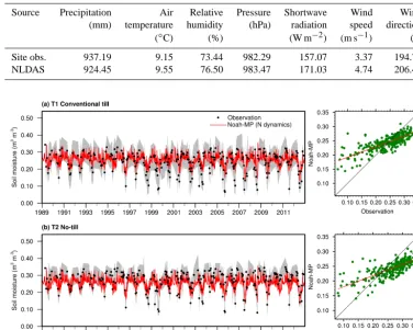
Figure 2. Observed and model-simulated volumetric soil moisture from 1989 to 2012 for (a) treatment 1 – cropland with conventional tillage – and (b) treatment 2: cropland without tillage. The grey shaded area shows the observational ranges from up to six replicates for each treatment.
tent with previous study by Cai et al. (2014b). The model-simulated multiple year averages are both 0.243 for the two treatments. These are very close to observations, which are 0.238 and 0.264 for T1 and T2, respectively. The correlation coefficient is 0.78 for T1 and 0.76 for T2, which are consid-ered high skills, especially on a daily scale.
However, differences between modeled and observed soil moisture are also found. From observation (Fig. 2), we can see that the treatment without tillage (T2) has slightly higher soil moisture than the treatment with tillage (T1). Therefore, tillage practice reduces soil moisture. However, the differ-ence in modeled soil moisture is negligible between the two treatments (both are 0.243). This is because Noah-MP does not consider water redistribution due to tillage, although N redistribution is considered in the soil N dynamic sub-model. N is redistributed by mixing a certain depth (i.e., 100 mm) of soil with a mixing efficiency (i.e., 30 %) (Neitsch et al., 2011). In addition, observed soil moisture has higher varia-tions. As we can see from Fig. 2, observation tends to have ei-ther higher peaks or lower valleys than model simulation. We also notice that some values from observation are extremely low, which may not be necessarily true in reality.
Consider-ing the wide spread of the observational ranges defined by up to six replicating plots, Noah-MP provides a reasonable water environment for the N cycling.
3.2 Evaluation of soil nitrate
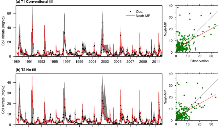
Soil nitrate concentration is the outcome of all N-related pro-cesses that occur in soil such as decomposition, mineraliza-tion, nitrificamineraliza-tion, denitrificamineraliza-tion, and uptake. It determines the available N that plants can use. The skills in modeling the soil nitrate concentration reflect the overall performance of the model in simulating the N cycle. Figure 3 shows the comparison of the model-simulated soil nitrate concentration with site observations for both T1 and T2. The model ctures the major variations of the soil nitrate. N fertilizer ap-plication is responsible for the high peaks. These high peaks drop very fast at first and then drop slowly, which can sustain crop growth for a few months.
Figure 3. Observed and model-simulated soil nitrate concentration from 1989 to 2011 for (a) treatment 1 – cropland with conventional tillage – and (b) treatment 2: cropland without tillage. The grey shaded area shows the observational ranges from up to six replicates for each treatment.
Table 3. Annual averages of Noah-MP-simulated major nitrogen fluxes and NPP. The NPP within the parentheses is from observation.
Treatment NPP Uptake Humus Residue Denitrification Leaching
(gC m−2) mineralization decomposition (gN m−2) (gN m−2)
(gN m−2) (gN m−2)
Passive Active Fixation Retranslocation (gN m−2) (gN m−2) (gN m−2) (gN m−2)
T1 432 (437) 6.18 0.90 2.88 0.50 3.79 12.30 10.48 7.19
T2 441 (471) 6.62 0.69 2.84 0.50 2.64 9.34 8.80 4.77
can see that soil N dynamics may be affected by a variety of complicated factors, which makes it difficult to model. Therefore, although the correlation coefficients are not con-sidered high skills relative to the soil moisture statistics, they are still reasonable.
While both treatments show very similar patterns (Fig. 3), T1 with conventional tillage tends to have higher soil nitrate concentration. This is understandable because tillage prac-tices redistribute water and nutrients in soil, which acceler-ates the N cycling. Table 3 shows annual averages of major N fluxes for both treatments. T1 has higher rates of humus min-eralization and residue decomposition, but, at the same time, it also has higher rates of denitrification and leaching. There-fore, it produces more N2O (a greenhouse gas) and more N runoff to rivers. Particularly, with higher N leaching, less soil nitrate is available for passive uptake by plants. As a result, plants need to acquire more N through active uptake.
3.3 Evaluation of nitrate leaching from soil bottom N leaching can be transported to rivers through surface and subsurface runoff and to groundwater through percola-tion from soil bottom. Only the last pathway is measured at this site. Figure 4 shows the comparison of concentra-tions of the leached solution from the soil bottom between model simulation and observation. The averaged concen-tration of N leaching from the soil bottom for T1 (T2) is 12.84 mg kg−1 (8.86 mg kg−1) from model simulation and 13.57 mg kg−1(9.26 mg kg−1) from observation. The corre-lation coefficients are 0.43 and 0.40 for T1 and T2, respec-tively. Although these skills may not be considered satisfac-tory, the model can still produce comparable results with ob-servation.
concentra-Figure 4. Observed and model-simulated nitrate leaching from bottom of soil profile from 1995 to 2013 for (a) treatment 1 – cropland with conventional tillage – and (b) treatment 2: cropland without tillage. The grey shaded area shows the observational ranges from up to six replicates for each treatment.
tion is also high. The combination of high water infiltration (due to the storm) and high soil nitrate concentration resulted in a large amount of soil nitrate being brought to the bottom soil layer. A few months following that, there was no large storm, which was again different from a normal year. As a result, the high-concentration nitrate solution was drained slowly out of the bottom layer of soil. The modeled nitrate leaching also shows a peak over this period, but the values are only close to the lower bound of the observed range. This suggests that improvement is needed so the model can better capture peaks under this situation.
We also notice that, without tillage, N leaching is about one-third lower than that with tillage. Without tillage, the temporal variation is also smaller.
3.4 Evaluation of annual NPP
NPP indicates the amount of C that is assimilated from the atmosphere into plants and thus is important in studying not only crop and ecosystem productivity but also climate change feedbacks. NPP is mainly determined by plant pho-tosynthesis and autotrophic respiration. It is also affected by water and nutrient stresses. In this study, N stress on plant growth is calculated by the reduction of NPP due to N acqui-sition, which can be considered another form of plant respi-ration. Figure 5 shows the comparison of simulated annual NPP against observation. Since the original Noah-MP with-out N dynamics also simulates NPP, its results are also shown here as a reference. The mean annual NPP simulated by the original Noah-MP is 544 gC m−2 (the same simulation for both treatments as original Noah-MP does not distinguish
tillage and no tillage). By including the N dynamics, simu-lated annual NPP is reduced to 432 gC m−2(441 gC m−2)for T1 (T2), which is more consistent with observed 437 gC m−2 (471 gC m−2). The correlation coefficient increased to 0.77 for T1, and from 0.30 to 0.72 for T2, which is a significant improvement. This improvement is due to the better charac-terization of the amount of carbon allocated to N acquisition instead of growth.
The modeled rate of NPP down-regulation – the fraction of NPP reduction due to N limitation – is 35.4 and 34.7 % for T1 and T2, respectively. These rates are close to the 33 % of down-regulation rate used in the default Noah-MP. By dy-namically simulating the demand and supply of N with time, these become even closer to the observations.
Surprisingly, even with slower N cycling, T2 produces slightly higher NPP (Table 3), which is consistent between model and observation. If this is the case, except for dry-ing up soil, releasdry-ing more N2O gas, and producing more N leaching, is there any benefit from tillage? The answer is yes. Less N fertilizer is needed for cropland with tillage. Based on the site management log, in total there was 194.8 gN m−2 of N fertilizer applied to T1 from 1989 to 2013, which is less than the amount (210.7 gN m−2)applied to T2 during the same period.
Figure 5. Observed and modeled annual NPP from 1989 to 2013 for (a) treatment 1 – cropland with conventional tillage – and (b) treatment 2: cropland without tillage. The error bars show the observational ranges from up to six replicates for each treatment.
The change in LAI can affect photosynthesis, which in return affects NPP.
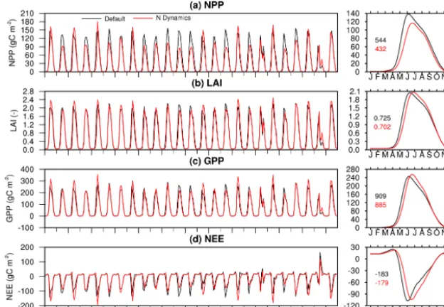
Figure 6 shows the comparison of the simulated C-related state and flux variables between the default and N dynam-ics enhanced Noah-MP. We can see that NPP is decreased from 544 to 432 gC m−2. Most of the decrease occurs be-fore the peak growing season, which results in a slight de-crease in LAI. However, the peak LAI has very minor in-crease. After the peak, LAI decreases more slowly than the default, which is due to the decreased turnover rate propor-tional to the NPP down-regulation rate. If the turnover rate is not down-regulated accordingly, the peak LAI will be cut in half. Due to the slower turnover rate, more leaf biomass (indicated by LAI) is involved in photosynthesis. Therefore, compared to the default, Noah-MP with N dynamics gener-ates higher gross primary production (GPP) during the sec-ond half of the growing season, although it is lower during the first half of the growing season. Annual mean GPP is de-creased by about 28 gC m−2.
Net ecosystem exchange (NEE) has a similar change. The annual NEE is−179 gC m−2(−183 gC m−2)from Noah-MP with N dynamics (default Noah-MP), which is comparable to the NEE in West et al. (2010) for this region. Its absolute value is decreased by 4 gC m−2, which means that the C sink is slightly decreased. This decrease is small compared to the GPP decrease, probably because soil respiration is also creased. All annual peaks of NPP, LAI, GPP, and NEE are de-layed for about half a month. This is probably due to the fact that the primary N fertilizations (>10 gN m−2)were mainly
applied after late June and thus plants encountered high N stress during the first half of the growing season.
3.6 Impacts of nitrogen dynamics on water cycle Through the changes in LAI and soil organic matters (SOMs), the addition of N dynamics affects not only the car-bon cycle but also the water cycle. The change in SOM is not currently considered, and therefore the impacts on the water cycle are from the change in LAI only, as shown in Fig. 7. These impacts are most pronounced on plant tran-spiration, which is increased by 33 mm yr−1. The increase mostly occurs during and after the peak growing season. In Cai et al. (2014a), Noah-MP-simulated evapotranspiration (ET) over croplands increases too fast during the first half of the growing season and reaches peak about 1 month ear-lier than observation. The delayed peaks of LAI and ET can partly mitigate this issue. As there is more water extracted from soil by transpiration, soil moisture further decreases during the second half of the growing season. Therefore, less water is available and thus soil evaporation is decreased by 9 mm yr−1. With the increase in ET, runoff is decreased by 13 mm yr−1.
Figure 6. (left column) Monthly and (right column) climatologically seasonal cycle of model-simulated (a) LAI, (b) NPP, (c) GPP, and (d) NEE from default Noah-MP and enhanced Noah-MP with N dynamics. The values in the right column indicate annual mean for each term (black: Noah-MP without N dynamics; red: Noah-MP with N dynamics).
Figure 7. Same as Fig. 6 except for (a) soil moisture, (b) transpiration, (c) soil evaporation, and (d) runoff.
3.7 Impacts of nitrogen fertilizer application
Observed N fertilizer application data are used in this study. However, this type of data is not always available, especially when models are applied in large regions. Often we only know the approximate amount of N fertilizer applied, with-out information on the exact dates. To guide the future large-scale application of this model, two additional experiments are run: (1) N fertilizer is applied on 20 June every year, and
(2) N fertilizer is applied on 15 April every year. The first experiment is designed because in this site a large amount of N fertilizer is applied mostly during mid-June and early July. Other dates are also reported in the literature; therefore, we use 15 April as another example. Both experiments use the same amount of N fertilizer as in the management log, which on average is 7.8 g N m−2yr−1.
Figure 8. (left column) Monthly and (right column) climatologically seasonal cycle of model-simulated (a) NPP, (b) N uptake, (c) N leaching, and (d) soil nitrate with different dates for N fertilization: real, 20 June, and 15 April. The values in the right column indicate annual mean for each term (black: real; red: 20 June; blue: 15 April). (e) Actual nitrogen fertilizer application amounts and dates as recorded in the agronomic log.
recorded dates and amount of N fertilizer application. De-spite the different application time, the two experiments pro-duce very consistent NPP with the real case. The 20 June experiment is much closer to the real case; even the seasonal variation is identical. The largest discrepancy is in 1993 and 1996. Based on the management log, in these two years, a large amount of N fertilizer was applied, which resulted in much higher NPP than results from the two experiments. Since 15 April is much earlier than the primary fertilizer application dates, NPP from this experiment is flattened out through the year. This also confirms the statement in Sect. 3.5 that later N fertilizer applications delay plant growth. Sim-ulated N uptake from both experiments shows exactly the same story as NPP.
The simulated N leaching shows the opposite pattern to NPP. The default simulation produces the highest leaching, followed by the 20 June experiment and then the 15 April ex-periment. This is very likely because the fertilizer application dates are closer to the flood season for the former two cases and the chance of fertilized N being flashed out is higher. The difference in N fertilization dates also clearly affects the sim-ulations of total soil nitrate. In the 20 June experiment, soil nitrate reaches the lowest level in May because no N
fertil-izer is applied before 20 June. In the default case, N fertilfertil-izer can actually be applied as early as April, but with a smaller amount before mid-June, which prevents the soil nitrate con-centration from getting too low. Besides a large amount of N fertilizer applied in later months, the other reason that the default simulation reaches the highest concentration of soil nitrate is because it produces higher NPP, which can be re-turned to soil for decomposition.
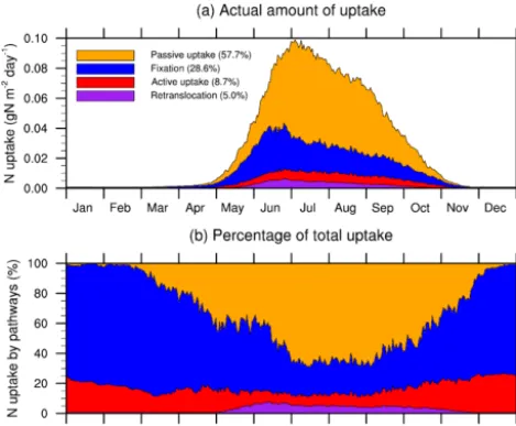
Figure 9. Daily climatology (1989–2013) of nitrogen uptake by pathways expresses as (a) actual amount of uptake and (b) percent-age of total uptake.
3.8 Analysis of nitrogen uptake
As described in Sect. 2.2.1, plants can get N for growth from four pathways: passive uptake, active uptake, fixation, and retranslocation, and the last three require C costs. Figure 9 shows the actual N uptake from these pathways and their percentages of contribution to the total N uptake. Passive up-take is the dominant pathway, which contributes 57.7 % of the total N uptake. Fixation, active uptake, and retransloca-tion contribute 28.6, 8.7, and 5.0 %, respectively. This con-trasts the results from the study by Brzostek et al. (2014) for non-fertilized trees, in which passive uptake only accounts for a small contribution. This is understandable because the purpose of fertilization is to minimize active uptake so that more NPP can be retained for crop growth. As demonstrated in Timlin et al. (2009), a higher fertilization rate results in a higher ratio of N uptake in transpiration to total N uptake. On the one hand, fertilization maintains soil nitrate concen-tration at high level. On the other hand, higher NPP for crop growth in turn results in higher LAI and thus higher transpi-ration. During peak growing season, therefore, plants receive a large amount of N under the combination of high transpira-tion and high soil nitrate concentratranspira-tion. During other periods, biological N fixation dominates.
3.9 Analysis of major soil nitrate fluxes
The soil nitrate storage with time is an outcome of the variations in incoming and outgoing fluxes. Besides N fer-tilizer and atmospheric deposition, humus mineralization and residue decomposition are the two major incoming fluxes. Because N fertilizer is a jumping behavior and atmo-spheric deposition is a relatively small fraction in this study
Figure 10. Daily climatology of the soil nitrate (blue solid line) and some major fluxes (color label bars) going in (humus mineralization and residue decomposition) and out (plant uptake, nitrate leaching, and denitrification) of the soil nitrate pool.
(∼1.5 gN m−2yr−1), they are not analyzed here. The major outgoing fluxes are denitrification, leaching, and plant up-take.
Figure 10 shows the seasonal variation of the above ma-jor fluxes. During the growing season, N fertilizer provides an important role in meeting the plant N demand; however, residue decomposition still makes the largest contribution and is the dominant factor responsible for the increase in total soil nitrate. During the non-growing season, a large amount of N is lost through denitrification and N leaching. However, when it reaches the peak growing season, plants consume a large fraction of soil nitrate, which leaves very little for denitrification and leaching. N leaching is mostly associated with the timing and intensity of precipitation. Denitrification is also associated with precipitation, but it is directly related to the soil water content. High denitrification rate occurs dur-ing high soil water content, especially durdur-ing water loggdur-ing.
4 Conclusions
In this study, a dynamic N model is coupled into Noah-MP by incorporating FUN’s strength in plant N uptake and SWAT’s strength in soil N cycling and agricultural management.
Moreover, the addition of N dynamics in Noah-MP im-proves the modeling of the carbon and water cycles. Com-pared to the default Noah-MP, NPP simulations are improved significantly, in terms of consistent averages and much higher correlation coefficients with observation. The temporal pat-tern of simulated ET is also improved, featuring lower ET during spring and delayed peak.
This enhancement is expected to facilitate the simultane-ous predictions of weather and environment by using a fully coupled Earth modeling system.
Code availability
Noah-MP is an open-source land surface model. The model is being developed by a community led by The University of Texas at Austin. The code is archived at both http://www. ral.ucar.edu/research/land/technology/noahmp_lsm.php and http://www.jsg.utexas.edu/noah-mp. The new code imple-mented in this study will be made available and may be ob-tained by contacting the corresponding author via email.
Acknowledgements. This work is supported by the NASA grant
NNX11AE42G, the National Center for Atmospheric Research Advanced Study Program, and the NASA Jet Propulsion Labo-ratory Strategic University Research Partnership Program. The first author would like to thank Guo-Yue Niu and Mingjie Shi for their help and the beneficial discussion with them. J. B. Fisher contributed to this research from the Jet Propulsion Laboratory, California Institute of Technology, under a contract with NASA, and through the University of California, Los Angeles. J. B. Fisher was supported by the US Department of Energy, Office of Science, Terrestrial Ecosystem Science program, and by the NSF Ecosystem Science program. X. Zhang’s contribution was supported by NASA (NNH11DA001N and NNH13ZDA001N). We are grateful for the observational data from the Kellogg Biological Station, which is supported by the NSF LTER Program (DEB 1027253), by Michigan State University AgBioResearch, and by the DOE Great Lakes Bioenergy Research Center (DE-FCO2-07ER64494 and DE-ACO5-76RL01830).
Edited by: A. B. Guenther
References
Boesch, D. F., Boynton, W. R., Crowder, L. B., Diaz, R. J., Howarth, R. W., Mee, L. D., Nixon, S. W., Rabalais, N. N., Rosenberg, R., Sanders, J. G., Scavia, D., and Turner, R. E.: Nutrient enrichment drives Gulf of Mexico hypoxia, EOS T. Am. Geophys. Un., 90, 117–118, doi:10.1029/2009eo140001, 2009.
Bonan, G. B.: Atmosphere-biosphere exchange of carbon dioxide in boreal forests, J. Geophys. Res., 96, 7301–7312, 1991. Bonan, G. B. and Levis, S.: Quantifying carbon-nitrogen feedbacks
in the Community Land Model (CLM4), Geophys. Res. Lett., 37, L07401, doi:10.1029/2010GL042430, 2010.
Boyer, E. W., Howarth, R. W., Galloway, J. N., Dentener, F. J., Green, P. A., and Vorosmarty, C. J.: Riverine nitrogen export
from the continents to the coasts, Global Biogeochem. Cy., 20, GB1S91, doi:10.1029/2005GB002537, 2006.
Brzostek, E. R., Fisher, J. B., and Phillips, R. P.: Modeling the car-bon cost of plant nitrogen acquisition: Mycorrhizal trade-offs and multipath resistance uptake improve predictions of retransloca-tion, J. Geophys. Res., 119, 1684-1697, 2014.
Cai, X., Yang, Z.-L., David, C. H., Niu, G.-Y., and Rodell, M.: Hy-drological evaluation of the Noah-MP land surface model for the Mississippi River Basin, J. Geophys. Res., 119, 23–38, 2014a. Cai, X., Yang, Z.-L., Xia, Y., Huang, M., Wei, H., Leung, L. R., and
Ek, M. B.: Assessment of simulated water balance from Noah, Noah-MP, CLM, and VIC over CONUS using the NLDAS test bed, J. Geophys. Res., 119, 13751–13770, 2014b.
Clark, D. B., Mercado, L. M., Sitch, S., Jones, C. D., Gedney, N., Best, M. J., Pryor, M., Rooney, G. G., Essery, R. L. H., Blyth, E., Boucher, O., Harding, R. J., Huntingford, C., and Cox, P. M.: The Joint UK Land Environment Simulator (JULES), model descrip-tion – Part 2: Carbon fluxes and vegetadescrip-tion dynamics, Geosci. Model Dev., 4, 701–722, doi:10.5194/gmd-4-701-2011, 2011. Clark, M. P., Kavetski, D., and Fenicia, F.: Pursuing the method of
multiple working hypotheses for hydrological modeling, Water Resour. Res., 47, W09301, doi:10.1029/2010wr009827, 2011. Conley, D. J., Paerl, H. W., Howarth, R. W., Boesch, D. F.,
Seitzinger, S. P., Havens, K. E., Lancelot, C., and Likens, G. E.: Controlling eutrophication: Nitrogen and phosphorus, Science, 323, 1014–1015, 2009.
Diaz, R. J. and Rosenberg, R.: Spreading dead zones and conse-quences for marine ecosystems, Science, 321, 926–929, 2008. Dickinson, R. E., Berry, J. A., Bonan, G. B., Collatz, G. J., Field,
C. B., Fung, I. Y., Goulden, M., Hoffmann, W. A., Jackson, R. B., Myneni, R., Sellers, P. J., and Shaikh, M.: Nitrogen controls on climate model evapotranspiration, J. Climate, 15, 278–295, 2002.
Donner, S. D. and Scavia, D.: How climate controls the flux of ni-trogen by the Mississippi River and the development of hypoxia in the Gulf of Mexico, Limnol. Oceanogr., 52, 856–861, 2007. Fisher, J. B., Sitch, S., Malhi, Y., Fisher, R. A., Huntingford, C.,
and Tan, S. Y.: Carbon cost of plant nitrogen acquisition: A mechanistic, globally applicable model of plant nitrogen up-take, retranslocation, and fixation, Global Biogeochem. Cy., 24, Gb1014, doi:10.1029/2009gb003621, 2010.
Fisher, J. B., Badgley, G., and Blyth, E.: Global nutrient limitation in terrestrial vegetation, Global Biogeochem. Cy., 26, Gb3007, doi:10.1029/2011gb004252, 2012.
Fowler, D., Coyle, M., Skiba, U., Sutton, M. A., Cape, J. N., Reis, S., Sheppard, L. J., Jenkins, A., Grizzetti, B., Galloway, J. N., Vitousek, P., Leach, A., Bouwman, A. F., Butterbach-Bahl, K., Dentener, F., Stevenson, D., Amann, M., and Voss, M.: The global nitrogen cycle in the twenty-first century, Philos. T. R. Soc. B, 368, 20130164, doi:10.1098/Rstb.2013.0164, 2013. Gruber, N. and Galloway, J. N.: An Earth-system perspective of the
global nitrogen cycle, Nature, 451, 293–296, 2008.
Houlton, B. Z., Wang, Y. P., Vitousek, P. M., and Field, C. B.: A unifying framework for dinitrogen fixation in the terrestrial bio-sphere, Nature, 454, 327–334, 2008.
Knops, J. M. H. and Tilman, D.: Dynamics of soil nitrogen and car-bon accumulation for 61 years after agricultural abandonment, Ecology, 81, 88–98, 2000.
Komatsu, E., Fukushima, T., and Harasawa, H.: A modeling ap-proach to forecast the effect of long-term climate change on lake water quality, Ecol. Model., 209, 351–366, 2007.
Kronvang, B., Behrendt, H., Andersen, H. E., Arheimer, B., Barr, A., Borgvang, S. A., Bouraoui, F., Granlund, K., Grizzetti, B., Groenendijk, P., Schwaiger, E., Hejzlar, J., Hoffmann, L., Johns-son, H., Panagopoulos, Y., Lo Porto, A., Reisser, H., Schoumans, O., Anthony, S., Silgram, M., Venohr, M., and Larsen, S. E.: En-semble modelling of nutrient loads and nutrient load partitioning in 17 European catchments, J. Environ. Monitor., 11, 572–583, 2009.
National Research Council: Clean coastal waters: understanding and reducing the effects of nutrient pollution, National Academy of Sciences, Washington, D.C., 2000.
Neitsch, S. L., Arnold, J. G., Kiniry, J. R., and Williams, J. R.: Soil and Water Assessment Tool theoretical documentation version 2009, Texas Water Resources Institute, Texas A&M University, College Station, TXTechnical Report No. 406, 2011.
Niu, G.-Y., Yang, Z.-L., Mitchell, K. E., Chen, F., Ek, M. B., Barlage, M., Kumar, A., Manning, K., Niyogi, D., Rosero, E., Tewari, M., and Xia, Y. L.: The community Noah land surface model with multiparameterization options (Noah-MP): 1. Model description and evaluation with local-scale measurements, J. Geophys. Res., 116, D12109, doi:10.1029/2010jd015139, 2011. Oleson, K. W., Lawrence, D. M., Bonan, G. B., Drewniak, B., Huang, M., Koven, C. D., Levis, S., Li, F., Riley, W. J., Subin, Z. M., Swenson, S. C., Thornton, P. E., Bozbiyik, A., Fisher, R., Heald, C. L., Kluzek, E., Lamarque, J.-F., Lawrence, P. J., Leung, L. R., Lipscomb, W., Muszala, S., Ricciuto, D. M., Sacks, W., Sun, Y., Tang, J., and Yang, Z.-L.: Technical description of ver-sion 4.5 of the Community Land Model (CLM), National Center for Atmospheric Research, Boulder, ColoradoNCAR Technical Note NCAR/TN-503+STR, 434 pp., 2013.
Prince, S. D., Haskett, J., Steininger, M., Strand, H., and Wright, R.: Net primary production of US Midwest croplands from agricul-tural harvest yield data, Ecol. Appl., 11, 1194–1205, 2001. Rasmussen, R., Ikeda, K., Liu, C. H., Gochis, D., Clark, M., Dai, A.
G., Gutmann, E., Dudhia, J., Chen, F., Barlage, M., Yates, D., and Zhang, G.: Climate change impacts on the water balance of the Colorado headwaters: High-resolution regional climate model simulations, J. Hydrometeorol., 15, 1091–1116, 2014.
Running, S. W. and Coughlan, J. C.: A general model of forest ecosystem processes for regional applications I. Hydrologic bal-ance, canopy, Ecol. Model., 42, 125–154, 1988.
Scanlon, B. R., Reedy, R. C., and Bronson, K. F.: Impacts of land use change on nitrogen cycling archived in semiarid unsaturated zone nitrate profiles, southern High Plains, Texas, Environ. Sci. Technol., 42, 7566–7572, 2008.
Schoumans, O. F., Silgram, M., Groenendijk, P., Bouraoui, F., An-dersen, H. E., Kronvang, B., Behrendt, H., Arheimer, B., Johns-son, H., Panagopoulos, Y., Mimikou, M., Lo Porto, A., Reisser, H., Le Gall, G., Barr, A., and Anthony, S. G.: Description of nine nutrient loss models: capabilities and suitability based on their characteristics, J. Environ. Monitor., 11, 506–514, 2009.
Shi, M., Fisher, J. B., Brzostek, E. R., and Phillips, R. P.: Carbon cost of plant nitrogen acquisition: global carbon cycle impact from an improved plant nitrogen cycle in the Community Land Model, Global Change Biol., doi:10.1111/gcb.13131, in press, 2016.
Thornton, P. E., Lamarque, J. F., Rosenbloom, N. A., and Mahowald, N. M.: Influence of carbon-nitrogen cycle cou-pling on land model response to CO2 fertilization and climate variability, Global Biogeochem. Cy., 21, Gb4018, doi:10.1029/2006gb002868, 2007.
Timlin, D., Kouznetsov, M., Fleisher, D., Kim, S.-H., and Reddy, V. R.: Simulation of nitrogen demand and uptake in potato using a carbon-assimilation approach, in: Quantifying and Understand-ing Plant Nitrogen Uptake for Systems ModelUnderstand-ing, edited by: Ma, L., Ahuja, L. R., and Bruulsema, T. W., CRC Press, 2009. Wang, Y. P., Houlton, B. Z., and Field, C. B.: A model of
biogeo-chemical cycles of carbon, nitrogen, and phosphorus including symbiotic nitrogen fixation and phosphatase production, Global Biogeochem. Cy., 21, Gb1018, doi:10.1029/2006gb002797, 2007.
West, T. O., Brandt, C. C., Baskaran, L. M., Hellwinckel, C. M., Mueller, R., Bernacchi, C. J., Bandaru, V., Yang, B., Wilson, B. S., Marland, G., Nelson, R. G., Ugarte, D. G. D. L. T., and Post, W. M.: Cropland carbon fluxes in the United States: increas-ing geospatial resolution of inventory-based carbon accountincreas-ing, Ecol. Appl., 20, 1074–1086, 2010.
Williams, J. R.: The EPIC model, in: Computer models of water-shed hydrology, edited by: Singh, V. P., Water Resources Publi-cations, Highlands Ranch, CO, 1995.
Xia, Y. L., Mitchell, K., Ek, M., Sheffield, J., Cosgrove, B., Wood, E., Luo, L. F., Alonge, C., Wei, H. L., Meng, J., Livneh, B., Lettenmaier, D., Koren, V., Duan, Q. Y., Mo, K., Fan, Y., and Mocko, D.: Continental-scale water and energy flux analysis and validation for the North American Land Data Assimilation Sys-tem project phase 2 (NLDAS-2): 1. Intercomparison and ap-plication of model products, J. Geophys. Res., 117, D03109, doi:10.1029/2011jd016048, 2012.
Yang, X. J., Wittig, V., Jain, A. K., and Post, W.: Integra-tion of nitrogen cycle dynamics into the Integrated Science Assessment Model for the study of terrestrial ecosystem re-sponses to global change, Global Biogeochem. Cy., 23, GB4029, doi:10.1029/2009gb003474, 2009.