https://doi.org/10.5194/gmd-11-1909-2018 © Author(s) 2018. This work is distributed under the Creative Commons Attribution 4.0 License.
Modeling soil CO
2
production and transport with dynamic source
and diffusion terms: testing the steady-state assumption
using DETECT v1.0
Edmund M. Ryan1,2, Kiona Ogle2,3,4,5, Heather Kropp6, Kimberly E. Samuels-Crow3, Yolima Carrillo7, and Elise Pendall7
1Lancaster Environment Centre, Lancaster University, Lancaster, UK 2School of Life Sciences, Arizona State University, Tempe, Arizona, USA
3School of Informatics, Computing, and Cyber Systems, Northern Arizona University, Flagstaff, Arizona, USA 4Center for Ecosystem Science and Society, Northern Arizona University, Flagstaff, Arizona, USA
5Department of Biological Sciences, Northern Arizona University, Flagstaff, Arizona, USA 6Department of Geography, Colgate University, Hamilton, New York, USA
7Hawkesbury Institute for the Environment, Western Sydney University, NSW, Australia
Correspondence:Edmund M. Ryan ([email protected]) Received: 7 September 2017 – Discussion started: 10 October 2017
Revised: 15 February 2018 – Accepted: 21 February 2018 – Published: 28 May 2018
Abstract. The flux of CO2from the soil to the atmosphere
(soil respiration,Rsoil)is a major component of the global
carbon (C) cycle. Methods to measure and model Rsoil, or
partition it into different components, often rely on the as-sumption that soil CO2 concentrations and fluxes are in
steady state, implying thatRsoil is equal to the rate at which
CO2is produced by soil microbial and root respiration.
Re-cent research, however, questions the validity of this assump-tion. Thus, the aim of this work was two-fold: (1) to de-scribe a non-steady state (NSS) soil CO2transport and
pro-duction model, DETECT, and (2) to use this model to evalu-ate the environmental conditions under whichRsoiland CO2
production are likely in NSS. The backbone of DETECT is a non-homogeneous, partial differential equation (PDE) that describes production and transport of soil CO2, which
we solve numerically at fine spatial and temporal resolution (e.g., 0.01 m increments down to 1 m, every 6 h). Production of soil CO2is simulated for every depth and time increment
as the sum of root respiration and microbial decomposition of soil organic matter. Both of these factors can be driven by current and antecedent soil water content and temperature, which can also vary by time and depth. We also analytically solved the ordinary differential equation (ODE) correspond-ing to the steady-state (SS) solution to the PDE model. We applied the DETECT NSS and SS models to the six-month
growing season period representative of a native grassland in Wyoming. Simulation experiments were conducted with both model versions to evaluate factors that could affect de-parture from SS, such as (1) varying soil texture; (2) shifting the timing or frequency of precipitation; and (3) with and without the environmental antecedent drivers. For a coarse-textured soil,Rsoil from the SS model closely matched that
of the NSS model. However, in a fine-textured (clay) soil, growing seasonRsoilwas∼3 % higher under the assumption
of NSS (versus SS). These differences were exaggerated in clay soil at daily time scales wherebyRsoilunder the SS
as-sumption deviated from NSS by up to 35 % on average in the 10 days following a major precipitation event. Incorpo-ration of antecedent drivers increased the magnitude ofRsoil
by 15 to 37 % for coarse- and fine-textured soils, respectively. However, the responses ofRsoilto the timing of precipitation
and antecedent drivers did not differ between SS and NSS assumptions. In summary, the assumption of SS conditions can be violated depending on soil type and soil moisture sta-tus, as affected by precipitation inputs. The DETECT model provides a framework for accommodating NSS conditions to better predictRsoil and associated soil carbon cycling
1 Introduction
The flux of CO2to the atmosphere from the soil (i.e., soil
res-piration,Rsoil)is one of the largest fluxes in the global carbon
(C) cycle, and when aggregated globally over an entire year it is approximately 10 times the annual amount of CO2emitted
by fossil fuel burning (Friedlingstein et al., 2014; Hashimoto et al., 2015). Moreover, global change experiments and pre-dictions from models agree thatRsoilis expected to increase
in a future climate of elevated CO2and warming (Cox, 2001;
Davidson and Janssens, 2006; Piao et al., 2009; Pendall et al., 2013; Ryan et al., 2015). Therefore, monitoringRsoil is
im-portant for quantifying and modeling the global C cycle. Commonly,Rsoil is monitored by directly measuring
sur-face soil CO2 fluxes using various chamber methods (Luo
and Zhou, 2010; Risk et al., 2011) or by estimatingRsoilfrom
soil CO2 concentrations measured at multiple depths using
probe methods (Pendall et al., 2003; Tang et al., 2003; Vargas et al., 2010). The probe methods employ diffusion equations that often rely on the assumption thatRsoilat the surface is in
steady state (SS) with subsurface CO2 production by roots
and micro-organisms (Tang et al., 2003; Lee et al., 2004; Baldocchi et al., 2006; Luo and Zhou, 2010; Vargas et al., 2010; Šim˚unek et al., 2012). That is, the SS assumption es-sentially presumes that CO2produced by roots and microbes
within the soil profile is instantaneously respired from the soil surface, effectively neglecting delays due to CO2
trans-port times. Partitioning Rsoil (surface flux) into its different
components (e.g., sub-surface heterotrophic [microbes] ver-sus autotrophic [root or rhizosphere] respiration) using iso-tope methods (Hui and Luo, 2004; Ogle and Pendall, 2015), trenching methods (Šim˚unek and Suarez, 1993), or soil CO2
models (Vargas et al., 2010) also relies on the SS assump-tion. Even simulations of the vertical movement of soil CO2
through snow have employed a SS diffusion model (Mon-son et al., 2006). Recent work, however, calls into question whether this SS assumption is valid most of the time or in most systems (Maggi and Riley, 2009; Nickerson and Risk, 2009).
Given the use of the SS assumption in a diverse range of settings, the aim of this study was to determine the meteo-rological and site specific conditions under which the SS as-sumption is valid, and the circumstances under which a non-steady state (NSS) model substantially improves our under-standing of subsurface processes that lead to observedRsoil.
We focused on soil texture because it is a critical factor un-derlying soil porosity and tortuosity, which, in turn, control soil CO2 diffusion rates (Bouma and Bryla, 2000). For
ex-ample, coarse-grained (e.g., high sand content) soils gener-ally facilitate fast CO2diffusion rates, especially under low
soil moisture conditions associated with high air-filled poros-ity (Bouma and Bryla, 2000); the opposite is expected for finer-grained (e.g., silt or clay) soils. Thus, we expect coarse-grained soils to generally induce SS conditions for soil CO2,
whereas fine-grained soils would likely produce frequent and
longer duration NSS conditions, especially following rain pulses that decrease air-filled pore space, thereby reducing CO2diffusivity.
We also focused on the impacts of precipitation variability given that the timing and magnitude of precipitation pulses can have large effects onRsoil(Huxman et al., 2004;
Schwin-ning et al., 2004; Sponseller, 2007; Cable et al., 2008; Borken and Matzner, 2009; Ogle et al., 2015). Precipitation indi-rectly impactsRsoilvia its influence on soil moisture
dynam-ics, and soil moisture and soil texture affect both diffusivity (a physical process) and CO2production (a primarily
biolog-ical process governed by roots and microbes). For example, as precipitation pulses infiltrate the soil, the CO2in the pore
spaces gets displaced with water, which may be seen as a transient spike inRsoil(e.g., Lee et al., 2004). Such transient
spikes, however, may also be attributable to changes in de-composition, microbial growth, and/or C substrate availabil-ity in response to wetting (Birch, 1958; Borken et al., 2003; Jarvis et al., 2007; Xiang et al., 2008; Meisner et al., 2013). This transient response may be followed by a depression in Rsoilsince water-filled pores will ultimately slow CO2
diffu-sion and transport (Bouma and Bryla, 2000). These linked effects imply that precipitation pulses and their effects on soil moisture are likely to impose NSS soil CO2conditions,
but the manner in which such pulses impact these processes is temporally dynamic and spatially complex, and therefore difficult to measure directly.
We evaluated the importance of soil texture and precipi-tation variability on SS versus NSS soil CO2 behavior via
a simulation-based approach. To allow for the possibility of both SS and NSS behavior, we implemented a depth- and time-varying CO2transport and production model that built
on the groundbreaking work of Fang and Moncrieff (1999), Hui and Luo (2004), Nickerson and Risk (2009), Moyes et al. (2010) and Risk et al. (2012). These processes are cap-tured by a partial differential equation (PDE) model that is grounded in diffusion theory, and solved numerically. Some current NSS models make simplifying assumptions such as assuming depth-invariant CO2 production rates (e.g., Fang
and Moncrieff, 1999), or assuming that production only re-sponds to concurrent environmental conditions (e.g., Nicker-son and Risk, 2009). Such simplifications may make it diffi-cult to evaluate physical and biological conditions leading to SS versus NSS behavior.
We addressed the aforementioned shortcomings of ex-isting NSS models with the DETECT (DEconvolution of Temporally varying Ecosystem Carbon componenTs) model, version 1.0 (v1.0), which implemented four improvements. First, we simulated soil CO2 at 100 different 0.01 m depth
increments to ensure numerical accuracy of the solutions (Haberman, 1998). Second, we estimated the soil water con-tent and soil temperature data for all depths and all time points using a separate model (HYDRUS; Šim˚unek et al., 2005, 2008). Third, we simulated the production of CO2
these processes to existing respiration models that are typi-cally applied to “bulk” soil (Lloyd and Taylor, 1994; Cable et al., 2008; Davidson et al., 2012; Todd-Brown et al., 2012). Fourth, we included antecedent (past) environmental and me-teorological conditions as part of the functions that predict soil CO2production, due to their importance for predicting
soil and ecosystem CO2 fluxes (Cable et al., 2013;
Barron-Gafford et al., 2014; Ryan et al., 2015). For example, soil respiration following a rain event is generally greater if the rain event follows a dry period versus a wet period (Xu et al., 2004; Sponseller, 2007; Cable et al., 2008, 2013; Thomas et al., 2008). Such antecedent effects may underlie the impor-tance of biological versus physical processes in governing the transition between SS and NSS behavior.
After describing the DETECT model, we subsequently use it to explore the effects of soil texture, precipitation pulses, and antecedent conditions on the relative importance of NSS soil CO2behavior and to identify the factors giving rise to
such behavior. We simulated soil CO2concentrations, CO2
production, and Rsoil under four different soil textures and
three different precipitation regimes. For each scenario, we implemented the DETECT model under the assumption that soil CO2production is affected by antecedent moisture and
temperature versus the assumption that only concurrent con-ditions matter. Data from the Wyoming Prairie Heating and CO2 Enrichment (PHACE) experiment (e.g., Pendall et al.,
2013; Carrillo et al., 2014a; Ryan et al., 2015; Zelikova et al., 2015; Mueller et al., 2016) were used to parameterize the model and motivated the selection of the texture and precipi-tation scenarios. Under the different scenarios, we compared Rsoilpredicted from the DETECT model to that of a simpler
SS model, and evaluated the relative impact of SS assump-tions on inferring subsurface processes (e.g., CO2production
by roots and microbes) and surface CO2fluxes (i.e.,Rsoil).
2 Methods
2.1 Description of the non steady state DETECT model
The PDE that underlies the DETECT model (v1.0) accounts for time- and depth-varying CO2diffusivity and CO2
produc-tion by root and microbial respiraproduc-tion (Fang and Moncrieff, 1999). We use a pair of PDEs, one describing the soil CO2
derived from root respiration (subscripted with R), and the other for CO2derived from microbial respiration (M) such
that forK=RorM: ∂cK(z, t )
∂t =
∂ ∂z
Dgs(z, t )
∂cK(z, t ) ∂z
+SK(z, t ). (1)
cK(z, t )is CO2concentration (mg CO2m−3),Dgs(z, t )is the
effective diffusivity of CO2 through the soil (m2s−1), and SK(z, t ) is the source (or production) term (mg CO2m−3)
(Fig. 1b), all of which vary by depthz(meters) and timet (hours). Note that Dgs is assumed to be the same for
root-and microbial-derived CO2 and is thus not indexed by K.
In this version of the model, we assumed that CO2
trans-port within the soil profile and over time is solely governed by gaseous diffusion, and we ignored other types of CO2
transport – such as diffusion in the liquid state, convection, and bulk transport via the vertical movement of water – that have been shown to have a negligible contribution (Fang and Moncrieff, 1999; Kayler et al., 2010). Total soil CO2and
to-tal CO2production are given asc(z, t )=cM(z, t )+cR(z, t ) andS(z, t )=SM(z, t )+SR(z, t ), respectively. Below we de-scribe the two main components of the PDE model: (1) CO2
diffusivity,Dgs, and (2) the production terms, SR(z, t ) and SM(z, t ). Finally, we note that Eq. (1) is the mass balance
equation (see Sect. S3 in the Supplement for more informa-tion).
2.1.1 Soil CO2diffusivity submodel
The diffusivity of CO2 within the soil (Dgs) depends on
the soil structure and water content; we modeled Dgs
us-ing the Moldrup function (Sala et al., 1992; Moldrup et al., 2004). We chose this formulation because it is more accu-rate than other common models, such as the Millington and Quirk (1961) and Penman (1940) models (Moldrup et al., 2004). Based on Moldrup et al. (2004),Dgs (m2s−1)is
de-fined as
Dgs(z, t )=Dg0(z, t )·
2φg100(z)3+0.04φg100(z)
·
φ
g(z, t ) φg100(z)
2+b(z)3
, (2)
where Dg0(z, t )=Dstp·
TS(z,t ) T0
1.75 · P0
P (t )
and Dstp=
1.39×10⁻⁵m2s−1 is the diffusion coefficient for CO2 in
air at standard temperature (T0, 273 K) and pressure (P0,
101.325 kPa); TS(z, t ) is the soil temperature (Kelvin) at depthz and timet, andP (t ) is the air pressure (kPa) just above the soil surface at time t. The remaining terms in Eq. (2) includeϕg(z,t ), the air-filled soil porosity, which is
related to the total soil porosity (ϕT)and volumetric soil
wa-ter content (θ ) according to ϕg(z, t )=ϕT(z)−θ (z, t ), and ϕT(z)is defined as 1−BD(z)/PD, where BD and PD are
the bulk density and particle density of the soil, respectively (Davidson et al., 2006);ϕg100(z)is the air-filled porosity at a
soil water potential (9)of −100 cm H2O (about−10 kPa); b(z)is a unitless parameter that is related to the pore size dis-tribution of the soil based on the water retention curve given by9=9e(θ/θsat)−b, where9e(z)is the air-entry potential
– calculated from measurements (Morgan et al., 2011) – and θsat(z)is the saturated soil water content (v/v).
2.1.2 CO2source (production) terms
Soil CO2can be produced in the soil (S term in Eq. 1) by
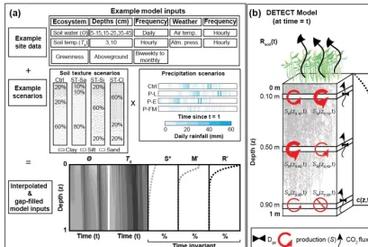
Figure 1.Graphical representation of(a)the required inputs to the DETECT model and the associated scenarios implemented in this study; and(b)the components of the DETECT model at a particular timet, indicating depth-dependent production, CO2concentrations, and CO2
fluxes.
rhizodeposits by root-associated microorganisms and associ-ated microbial respiration, (iv) microbial decomposition of newly produced plant litter that has been incorporated into the soil matrix, and (v) microbial decomposition of older soil organic matter (SOM) (Pendall et al., 2004). Due to the gen-eral lack of sufficient data and process understanding to ac-curately separate all five sources, the DETECT model treats CO2production as the sum of two main contributions: CO2
respired by (1) roots and closely associated microorganisms (the sum of i–iii), givingSR(z, t ), and (2) free-living soil mi-croorganisms (the sum of iv–v), givingSM(z, t ). Such
sim-plification based on root and microbial sources is common in models of soil CO2 transport and production (Šim˚unek
and Suarez, 1993; Fang and Moncrieff, 1999; Hui and Luo, 2004). Although DETECT v1.0 assumes that root and mi-crobial respiration are independent of one another, they both depend on the same environmental data (e.g.,θandTS).
CO2 production by root respiration is represented as the
product of three terms: (i) the mass-specific base respira-tion rate (RRbase)at a reference soil temperature ofTS=Tref
and at average soil water and antecedent conditions,(ii) root mass expressed as the amount of root carbon, CR(z, t ), and (iii) functions that rescaleRRbaseto account for the effect of
soil water (θ ), temperature (TS), and their antecedent coun-terparts. Antecedent temperature is denoted by TSant, and for roots antecedent soil water is given by θRant. In general,
SR(z, t )is given by
SR(z, t )=RRbase·CR(z, t )·f θ (z, t ) , θRant(z, t )
·g TS(z, t ) , TSant(z, t )
. (3)
The functional form of CR(z, t )is informed by field data on root biomass C (see Sect. S1 for complete details). The functionsf andgare given by
f θ, θRant=exp α1θ (z, t )+α2θRant(z, t ) +α3θ (z, t )·θRant(z, t )
(4a) g TS, TRant
=exp(Eo(z, t )
·
1
Tref−To
− 1
TS(z, t )−To
Tucker et al., 2013); we assumeEoresponds to antecedent temperature, reflecting a potential thermal acclimation re-sponse (Atkin and Tjoelker, 2003; Ryan et al., 2015).Tois also related to the apparent temperature sensitivity (Cable et al., 2011), and we assume that it is invariant with depth and time (Lloyd and Taylor, 1994; Cable et al., 2013; Barron-Gafford et al., 2014; Ryan et al., 2015). While the functional forms and choice of environmental drivers used for f and g were motivated by previous analyses (Cable et al., 2013; Barron-Gafford et al., 2014), the exact functions and param-eter values were based on Ryan et al. (2015) and Cable et al. (2013). Exponential functions are also used for the mois-ture (f) and temperature (g)scale functions to ensuref >0 and g >0 (Eq. 4a). The choice of an exponential form of the functions was based on Ryan et al. (2015), with graph-ical forms of the total CO2production based on these
func-tions given in Fig. S10 (Supplement). However, the DETECT model is flexible enough to accommodate alternative func-tions forf andg. For example, we ran DETECT for the con-trol scenario using a bell-shaped function that described how soil CO2production changes with θ (Sect. S4 and Fig. S8,
Supplement) as an alternative to Eq. (4a). For this alternative model run, the modeledRsoilwas very similar to the modeled Rsoilfrom the results of this study (Fig. S9, Supplement).
CO2 production by microbial respiration and SOM
de-composition is represented by a modified version of the Dual Arrhenius and Michaelis–Menten (DAMM) model (David-son et al., 2012). We exclude the O2 term, rendering the
model relevant to systems that are typically unlimited by O2
availability, such as the semi-arid site that we focus on, but we accounted for a microbial C pool (CMIC)and a soluble
soil-C pool (CSOL)(Todd-Brown et al., 2012) such that
SM(z, t )=Vmax(z, t )·
CSOL(z, t ) Km+CSOL(z, t )
·CMIC(z, t )·(1−CUE). (5)
Decomposition is assumed to be an enzymatic process that follows Michaelis–Menten kinetics, where Vmax is the
maximum potential decomposition rate, and Km (the
half-saturation constant) is the amount of substrate required for the decomposition rate to reach half ofVmax. Carbon-use
effi-ciency (CUE) represents the proportion of total C assimilated by microbes that is allocated for microbial growth (Tucker et al., 2013). We excluded a microbial death rate term (Todd-Brown et al., 2012) because we had insufficient data on death rates, and CMICis only∼1 % of CSOLat our study site
(Car-rillo and Pendall, 2018).
In contrast to the original DAMM formulation, we allowed SM(z, t )andVmax(z, t )to vary by depth and time, whereas
existing applications of the DAMM model are generally ap-plied to “bulk” soil (i.e., do not vary withz). We also mod-eled Vmax according to the modified energy of activation
function described in Lloyd and Taylor (1994), which
essen-tially parallels Eq. (4b)–(4c): Vmax(z, t )=VBase·f θ, θMant
·exp(Eo(z, t )
·
1
Tref−To
− 1
TS(z, t )−To
. (6)
VBaseis the “base”Vmaxat a reference soil temperature ofTref
and at mean values of currentθand antecedentθandTS(i.e., mean values ofθMantandTSant).Eo(z, t )andf θ, θmant
follow the same functional forms and interpretation as described for the root respiration submodel (Eqs. 3 and 4a–c), except that θMantis used instead ofθRant, respectively, and different values are specified for the parametersα1,α2,α3,α4,To, andEo∗to reflect microbial respiration The values are given in Table 1, and Sect. 2.4.5 explains how the values were estimated.
Finally, CSOL is modeled as a function of soil organic C
content at depth z, CSOM(z) based on the fraction, p, of
CSOM(z)that is soluble and the diffusivity of the substrate in
liquid,Dliq(Davidson et al., 2012). The equation for CSOLis
given by
CSOL(z, t )=CSOM(z)·p·θ (z, t )3·Dliq. (7)
The values ofpandDliqwere taken from laboratory
anal-ysis (see Sect. 2.4.5) and Davidson et al. (2012), respectively. We assumed that CSOM(z)and CMIC(z)(see Eq. 5) are
con-stant over time given the relatively short simulation peri-ods explored here (a single growing season); but the model could easily be modified to allow for time-varying CSOM
and CMIC. Here, CSOM(z)and CMIC(z)are simple,
empiri-cal functions that were informed by data (see Sect. S1 for de-tails). Moreover, while assumption of time invariant CSOM(z)
and CMIC(z)is an implicit SS assumption about biological
factors affecting soil CO2dynamics, this assumption allows
us to isolate the importance of NSS conditions that are pri-marily due to physical CO2transport characteristics.
2.1.3 Soil respiration
The efflux of CO2 from the soil surface (soil respiration, Rsoil)is computed as
Rsoil(t )=
Dgs(z=0.01, t )
1z (c(z=0.01, t )−catm(t )) . (8) Dgs(z=0.01, t ) is the diffusivity of CO2 in the soil and c(z=0.01, t )is the total CO2concentration (microbial- and
root-derived), respectively, atz=0.01 m depth and timet; catm(t )is the CO2concentration in the atmosphere above the
soil surface; and1zis the depth increment that the model solves for soil CO2concentration (here,1z=0.01 m).
2.2 Numerical implementation of the DETECT model
Table 1.Summary of scalar parameters used in the non-steady-state (DETECT) model, arranged into four groups: parameters unique to the microbial respiration submodel forSM(z, t )(group 1); parameters unique to the root respiration submodel forSR(z, t )(group 2); parameters
that are shared between theSM(z, t )andSR(z, t )submodels (group 3); parameters used to calculate soil CO2diffusivity,Dgs(group 4). See
Sect. 2.4.5 for details about how the parameters were estimated.
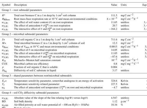
Symbol Description Value Units Eq(s).
Group 1 – root submodel parameters
R* Total root biomass C in a 1 m deep by 1 cm2soil column 111.5 mg C cm−2 3
RRBase Root mass-base respiration rate at 10◦C and mean environmental conditions 6×10⁻⁵ mg C cm−3h−1 3
α1(R) The effect of soil water content (θ )on root respiration 11.65 unitless 3, 4a
α2(R) The effect of antecedentθ(θRant)on root respiration 20.7 unitless 3, 4b
α3(R) The interactive effect ofθandθRanton root respiration −164.2 unitless 3, 4c
Group 2 – microbial submodel parameters
S∗ Total soil organic C in a 1 m deep by 1 cm2soil column 711.6 mg C cm−2 5
M∗ Total microbial biomass C in a 1 m deep by 1 cm2column of soil 12.3 mg C cm−2 5
VBase Value ofVmaxat 10◦C and mean environmental conditions 0.0015 mg C cm−3h−1 5, 6
α1(M) The effect ofθon microbial respiration 14.05 unitless 5, 6
α2(M) The effect of antecedentθ(θMant)on microbial respiration 11.05 unitless 5, 6
α3(M) The interactive effect ofθandθManton microbial respiration −87.6 unitless 5, 6
Km Michaelis–Menten half saturation constant 10−5 mg C cm−3h−1 5
CUE Microbial carbon-use efficiency 0.8 mg C mg−1C−1 5
p Fraction of soil organic C that is soluble 0.004 – 7
Dliq Diffusivity of soil C substrate in liquid 3.17 unitless 7
Group 3 – shared parameters between root/microbial submodels
Eo∗ Temperature sensitivity parameter, somewhat analogous to an energy of activation 324.6 Kelvin 4c
To Temperature sensitivity-related parameter 227.5 Kelvin 4c
α4 The effect of antecedent soil temperature (TSant)on root and microbial respiration −4.7 unitless 4c
Group 4 – soil CO2diffusivity submodel parameters
α3(R) Absolute value of the slope of the line relating log(9)versus log(θ ) 4.547 unitless 2
BD Soil bulk density 1.12 g cm−3 2
ϕg100 Air-filled porosity at soil water potential of−100 cm H20 (∼10 kPa) 18.16 % 2
PD Particle density
condition (IC) and two boundary conditions (BCs), which we specified as
IC: c (z, t=0)=c0(z) (9a)
Upper BC: c (z=0, t )=catm(t ) (9b)
Lower BC: ∂c(z=1, t )
∂z =0. (9c)
The function c0(z)is determined and parameterized in two
stages: (1) observed soil CO2 concentration data at three
depths from the start of the 2007 growing season were used to parametrize a simple function that described the change in CO2concentration for all depths; (2) the DETECT model
was run forward for the growing season of 2007, then the modeled CO2 concentrations for all depths on the final day
of the 2007 growing season (31 September 2007) was used as the initial condition for running the DETECT model for 2008. See Sect. S2 in the Supplement for specific details. We setcatm(t )equivalent to 356 ppm for allt, which was the
av-erage near-surface, ambient atmospheric CO2concentration
measured at the PHACE site in the 2008 growing season. Following the methods of Haberman (1998), we adopted a zero-flux lower BC (Eq. 9c) due to the lack of data at or near a depth of 1 m.
Prior to solving the non-linear PDE (Eq. 1), we expanded the RHS of Eq. (1) using the “product rule for differentia-tion”. We then numerically solved the non-linear PDE (Eq. 1) by employing a forward Euler discretization with a centered difference method for the depth derivative at a depth incre-ment of1z=0.01 m. To ensure numerical stability, we cal-culate model outputs at a numerical time step of1t= dt
Ndt, where dt is the time step at which the predicted outputs are stored (6 h), andNdt is the number of numerical time steps. Ndtis computed based on the fastest (largest) diffusion coef-ficient at each time step such thatNdt= dt×max(Dgs)
0.5×(1z)2 , where
max(Dgs)is the maximumDgs across all depth increments
both root- and microbial-derived CO2 concentrations, such
that forK=RorM: cK(z, t+1t )−cK(z, t )
1t =Dgs(z, t )
cK(z+1z, t )−2cK(z, t )+cK(z−1z, t )
(1t )2
+
D
gs(z+1z, t )−Dgs(z−1z, t )
21z
c
K(z−1z, t )−cK(z+1z, t ) 21z
+SK(z, t ) . (10)
We rearranged Eq. (10) to solve for cK(z, t+1t ), which was iterated forward for all time steps and depth increments; total CO2concentration at each time step and depth is
cal-culated asc(z, t+1t )=cR(z, t+1t )+cM(z, t+1t ). For
clarity, we emphasize that Eq. (10) is the discretized version of Eq. (1), which we require in order to numerically solve Eq. (1) (Haberman, 1998). We programmed the DETECT model v.10 and the numerical solution method in Matlab (Mathworks, 2016).
2.3 Steady-state (SS) solution to the DETECT model
A primary goal of this work was to test if soil CO2and
asso-ciatedRsoilpredicted from the non-steady-state (NSS) model
(DETECT) could be distinguished from that of the steady-state (SS) solution. The SS version of Eq. (1), which we refer to as the SS-DETECT model, can be solved analyti-cally as an ordinary differential equation (ODE) by setting the∂c/∂zterm to zero (Amundson et al., 1998). As with the NSS model, we found the SS solution to Eq. (1) separately for root- and microbial-derived CO2concentrations,c∗R(z, t )
andcM∗(z, t ), respectively. Using the upper and lower bound-ary conditions described for the NSS model (Eq. 9b and c), the analytical SS solutions at timet and depthzare derived by Amundson et al. (1998) and Cerling (1984). The solution is given by
c∗K(z, t )= S
∗
K(t ) Dgs(z, t )
z−z
2
2
+catm(t ) (11)
S∗K(t )= 1
100
1 m X
z=0.01
SK(z, t ), (12)
whereK=R andK=M refers to the soil CO2 from root
(R) and microbial (M) sources, respectively. SK∗(t ) is the depth-averaged source term for microbial or root production (averaging over 100 different 0.01 m increments). The soil CO2 diffusivity term,Dgs(z, t ), and upper boundary
condi-tion,catm(t ), are the same as previously defined (Eqs. 2 and
9b, respectively; Amundson et al., 1998).
2.4 Application of the DETECT and SS-DETECT models to the PHACE site
In this subsection, we provide an overview of the study site, including the PHACE experiment, and relevant data sources from PHACE that we used to drive the DETECT and SS-DETECT models. We also summarize how we calibrated the models in the context of the PHACE site, and we highlight data that we used to informally validate the general behavior of the models. We conclude by describing the simulation ex-periments that we conducted to test the effects of soil texture and precipitation variability on the importance of NSS versus SS soil CO2conditions.
2.4.1 Field site and PHACE experiment
The Prairie Heating and CO2 Enrichment (PHACE) field
experiment is located in south-central Wyoming (latitude 41◦500N, longitude 104◦420W, elevation 1930 m). The site is a mixed-grass prairie with a semi-arid climate character-ized by long winters (mean January temperature= −2.5◦C) and warm summers (mean July temperature = 17.5◦C), with mean annual precipitation of 384 mm (Morgan et al., 2011). The vegetation is predominantly composed of two C3grasses, western wheatgrass (Pascopyrum smithii(Rydb.)
A. Löve) and needle-and-thread grass (Hesperostipa comata
(Trin. & Rupr.)), and a C4 perennial grass, blue grama
(Bouteloua gracilis(H.B.K.) Lag). The soil is a fine-loamy, mixed, mesic Aridic Argiustoll, and biological crusts are not present (Bachman et al., 2010).
2.4.2 Environmental driving data
We simulated the transport and production of soil CO2 for
each 0.01 m depth increment, from the surface (0 m) to a depth of 1 m, across all 732 time steps (i.e., four time steps per day [every 6 h] for 183 days from April to September). To do this, we required soil environmental data consisting of wa-ter content (θ )and temperature (TS)and meteorological data including precipitation, air temperature, and air pressure. The θ andTS data that were used to drive the DETECT model were created using the HYDRUS software (see Sect. 2.4.3), calibrated against actual measurements ofθandTS. For the meteorological data, actual measurements from the PHACE site were used.
The PHACE experiment involved an incomplete factorial of CO2, warming, and irrigation (six treatment levels total),
with five replicate plots per treatment level, resulting in a to-tal of 30 instrumented plots. One of the five plots from the control treatment – ambient CO2, temperature (no heating),
and precipitation (no supplemental irrigation) – was chosen at random and had a system installed to measure soil CO2
we used were collected during the growing season (March– September) of 2008;θwas measured hourly at three depths (5–15, 15–25, and 35–45 cm; EnvironSMART probe, Sentek Sensor Technologies, Stepney, Australia) and we used daily averages to drive the models.TSwas measured hourly at two depths (3 and 10 cm) using type-T thermocouples. Hourly precipitation (mm), air temperature (◦C), relative humidity (%), and surface barometric air pressure (kPa) were recorded by an automated weather station at the site.
2.4.3 High-resolution environmental data
To accommodate the 0.01 m depth increments specified for the DETECT model, we used the coarse-resolution field data (above) to create finer-resolution driving data. For example, temporal gap-filling of the θ, TS, and micrometeorological datasets was required due to gaps that occurred during a small number of days (<1, 6, and 2.5 %, respectively) as a result of instrument failure. We used data from other nearby plots to estimate the values of the missing data, but we also used cubic spline interpolation where gaps remained. De-tails of these gap-filing methods can be found in Ryan et al. (2015).
We used HYDRUS-1D v4.16.0090 to simulateθandTSin 0.01 m increments from a depth of 0.01 to 1 m (Chou et al., 2008; Šim˚unek et al., 2008; Piao et al., 2009) based on pre-cipitation data at the site. HYDRUS simulates the movement of water by solving the Richards’ equation for water move-ment (Richards, 1931; Chou et al., 2008; Sitch et al., 2008) and heat transport via Fickian based advection–dispersion equations. Soil hydraulic and heat transport parameters were estimated in HYDRUS using the inverse mode to solve for parameter values based on the PHACEθ(5–10, 15–25, and 35–45 cm) andTS (3 and 10 cm) data (Šim˚unek et al., 2005, 2008). HYDRUS was then run in forward mode based on the tuned soil hydraulic parameters to estimateθ andTS at all 100 different 0.01 m depth increments at six-hourly time intervals. For consistency, HYDRUS-derivedθandTS were used as the environmental input data to the DETECT models, even at the depths for which PHACE data were available. 2.4.4 Antecedent soil water and soil temperature
conditions
We explicitly evaluated the impact of antecedent (past)θand TSconditions on CO2production by roots and microbes,
mo-tivated by prior work that estimated the relative importance of antecedent conditions and their time scales of influence on soil and ecosystem CO2efflux (Cable et al., 2013;
Barron-Gafford et al., 2014; Ogle et al., 2015; Ryan et al., 2015). Antecedent soil water content and antecedent soil tempera-ture –θKant(z, t )andTSant(z, t ), respectively, forK=R(roots) andM (microbes) were computed as weighted averages of the HYDRUS-produced θ (z, t ) and TS(z, t ) data, respec-tively. These calculations were done external to the DETECT
model, and the antecedent variables were supplied as driving variables to DETECT. For example, for each 0.01 m incre-ment (z)and time period (t ), antecedent soil water associated with microbial CO2production was calculated as
θMant(z, t )=
J X
j=1
w(j )·θ (z, t−j ). (13)
Thew’s are the antecedent importance weights, which sum to 1 fromj=1 (previous time period) toj=J (J previous time periods). The weights were informed by results from an analysis of ecosystem respiration at the PHACE site (Ryan et al., 2015). For microbes,J=4 days andw=(0.75, 0.25, 0, 0), indicating the strong importance ofθconditions occur-ring the previous day (j =1) (Oikawa et al., 2014). Similar equations were used to computeθRant(z, t )andTSant(z, t ), each with their own set of weights (w’s) and time scales (J’s). For example, the time step andJ for θ differ among microbes (2 days) and roots (3 weeks); for roots,θRant(z, t )was com-puted as a weighted average of past, average weekly values ofθ, withj denoting weeks into the past, forJ=4 weeks, andw=(0.2, 0.6, 0.2, 0), indicating a strong lag response toθconditions occurring two weeks ago (Cable et al., 2013; Ryan et al., 2015). For antecedent soil temperature, we as-sumed that each of the past four days were equally important by setting thewvectors to (0.25, 0.25, 0.25, 0.25), for both microbes and roots (Ryan et al., 2015). The specification ofJ and thew’s are independent of the DETECT model formula-tion and can be varied by the user. For clarity we summarize these weight parameters in Table 2.
2.4.5 Overview of parameterization approach using PHACE data
In general, our aim was to specify realistic values for the pa-rameters in the DETECT model. We did not formally “fit” the DETECT model to data, but rather, we simply deter-mined reasonable values based on simple analyses of rele-vant PHACE data sets, results published for the PHACE site, or results from other relevant studies. The full list of param-eters is given in Table 1, and below we describe the logic behind specifying the values in Table 1.
The depth-distributions of root biomass C (CR, Eq. 3), soil microbial biomass C (CMIC, Eq. 5), and soil organic C
(CSOM, Eq. 7) are expressed in terms of a total C content
in a 1 m deep soil column (R*, M*, and S*, respectively; mg C cm−2), multiplied by the proportion of that C that
oc-curs at depthz(fR(z),fM(z), andfS(z), respectively). See Sect. S1 (Supplement) for details. Regarding the data, soil organic C (Fig. S5, Supplement) was determined by combus-tion of acidified, root-free soil collected from 0–5, 5–15, 15– 30, 30–45, 45–75, and 75–100 cm depths, using a Costech Elemental Analyzer. Microbial biomass C was determined by the chloroform fumigation and extraction in 0.05 M K2SO4
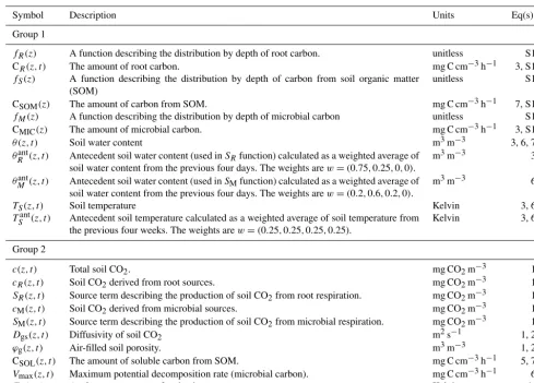
Table 2.Summary of quantities in the non-steady-state (DETECT) model that vary by depth only (z), or by depth (z)and time (t ). Those in group 1 represent input variables (derived prior to the running of the DETECT model), while group 2 contains the modeled quantities (used as part of the operation of the DETECT model). Equation (S1) can be found in Sect. S1 in the Supplement.
Symbol Description Units Eq(s).
Group 1
fR(z) A function describing the distribution by depth of root carbon. unitless S1
CR(z, t ) The amount of root carbon. mg C cm−3h−1 3, S1
fS(z) A function describing the distribution by depth of carbon from soil organic matter
(SOM)
unitless S1
CSOM(z) The amount of carbon from SOM. mg C cm−3h−1 7, S1
fM(z) A function describing the distribution by depth of microbial carbon unitless S1
CMIC(z) The amount of microbial carbon. mg C cm−3h−1 3, S1
θ (z, t ) Soil water content m3m−3 3, 6, 7
θRant(z, t ) Antecedent soil water content (used inSRfunction) calculated as a weighted average of
soil water content from the previous four days. The weights arew=(0.75,0.25,0,0).
m3m−3 3
θMant(z, t ) Antecedent soil water content (used inSMfunction) calculated as a weighted average of
soil water content from the previous four days. The weights arew=(0.2,0.6,0.2,0).
m3m−3 6
TS(z, t ) Soil temperature Kelvin 3, 6
TSant(z, t ) Antecedent soil temperature calculated as a weighted average of soil temperature from the previous four weeks. The weights arew=(0.25,0.25,0.25,0.25).
Kelvin 3, 6
Group 2
c(z, t ) Total soil CO2. mg CO2m−3 1
cR(z, t ) Soil CO2derived from root sources. mg CO2m−3 1
SR(z, t ) Source term describing the production of soil CO2from root respiration. mg CO2m−3 1
cM(z, t ) Soil CO2derived from microbial sources. mg CO2m−3 1
SM(z, t ) Source term describing the production of soil CO2from microbial respiration. mg CO2m−3 1
Dgs(z, t ) Diffusivity of soil CO2 m2s−1 1, 2
ϕg(z, t ) Air-filled soil porosity. m3m−3 1, 2
CSOL(z, t ) The amount of soluble carbon from SOM. mg C cm−3h−1 5, 7
Vmax(z, t ) Maximum potential decomposition rate (microbial carbon). mg C cm−3h−1 6
Eo(z, t ) Analogous to energy of activation. Kelvin 4c
on a total organic carbon analyzer (Shimadzu TOC-VCPN; Shimadzu Scientific Instruments, Wood Dale, IL, USA) af-ter treating with 1 M H3PO4 (1 µL per 10 mL of extract) to remove any carbonates. Root biomass C was estimated from ash-free root biomass and elemental analysis (Carrillo et al., 2014a; Mueller et al., 2016). The solubility parameter,p, was estimated as the ratio of CSOLto CSOMusing measurements
of these two quantities which were based on unfumigated ex-tracts obtained for microbial biomass estimations as above (CSOL)and on totalCconcentration in soil (CSOM).
The values used for the base microbial respiration rates and the half-saturation constant (VBase [Eq. 6] and Km
[Eq. 5]; Table 1) were estimated by fitting the microbial respiration submodel, but without the CMIC or CUE terms
(Eq. 5), to microbial respiration data from the PHACE con-trol plots (Fig. S7, Supplement). The CMIC and CUE terms
were not included in this earlier version of SMsubmodel –
which was used for model calibration purposes – because we did not have measurements of these two variables at the time. We estimated VBase andKm using a Markov chain Monte
Carlo approach, identical to the approach used in Ryan et al. (2015). In the absence of root respiration data, we as-sumed that base root respiration (RRbase [Eq. 3]; Table 1)
was proportional to the microbial base rate term (Hanson et al., 2000). The parameters denoting the effects of current soil moisture (e.g.,α1; Eq. 4a), antecedent moisture (α2), and
the interaction between current and antecedent moisture (α3)
on root and microbial respiration were derived from Ryan et al. (2015), based on an analysis of ecosystem respiration (Reco)data from PHACE. However, we adjusted the values
(Table 1) by trial and error to reflect the expectation that the effects of current soil moisture should be stronger for mi-crobial compared to root respiration because microbes tend to respond more rapidly to precipitation pulses (Risk et al., 2008), whereas root respiration is likely to show a delayed response which depends more strongly on past moisture con-ditions (Cable et al., 2008, 2013). Of the remaining two pa-rameters describingSM(Eqs. 5–6; Table 1), the value of CUE
Dliq was taken from Davidson et al. (2012). Three
parame-ters (Eo∗,To, andα4; Eq. 4a–b) were shared between theSR andSMsubmodels, and their values were also obtained from
Ryan et al. (2015). Finally, the parameters used for CO2
dif-fusivity (b, BD, andϕg100; Eq. 2) were based on published,
site-specific data (Morgan et al., 2011).
2.4.6 Informal model validation with soil respiration measurements
We evaluated the accuracy of the DETECT model by com-paring (1) predicted Rsoil (Eq. 8) against plot-level
mea-surements of ecosystem respiration (Reco)(see below) and
(2) predicted soil CO2 concentrations, c(z, t ), versus
ob-served concentrations; all obob-served data were from the PHACE study. Since we did not rigorously parameterize the DETECT model with PHACE data, we were simply looking for reasonable, qualitative agreement between the modeled variables and the observations (e.g., similar order of magni-tude, comparable temporal trends). ObservedRecowas
mea-sured on control plots every two to four weeks during the target growing season, using a canopy gas exchange cham-ber, and instantaneous fluxes were scaled to daily rates us-ing a linear, empirical function (Jasoni et al., 2005; Bach-man et al., 2010). We assumed thatRsoilwas similar toReco
given that aboveground biomass was <20 % of total plant biomass (Mueller et al., 2016). Measurements of microbial respiration were obtained by applying glyphosate herbicide to small subplots in May 2008, limiting ecosystem CO2
ef-flux to microbial sources (Pendall et al., 2013), Non-steady state soil chambers were used to estimate the resulting sur-face soil fluxes every two weeks around midday (Oleson et al., 2013; Ogle et al., 2016). Soil CO2 concentrations were
also measured with non-dispersive infrared sensors (Vaisala GM222, Finland) installed at 3, 10, and 20 cm below the soil surface, averaged on an hourly basis (Risk et al., 2008; Var-gas et al., 2011; Brennan, 2013). Observations of soil [CO2]
for control plots were compared against predictions ofc(z, t ) atz=0.03, 0.1, and 0.2 m and at the corresponding times. 2.5 Simulation experiments
We evaluated the impact of three potentially important fac-tors that could affect the frequency of NSS (Eqs. 1 and 9a–c) relative to SS (Eq. 11) conditions: (1) soil texture, (2) pre-cipitation patterns, and (3) importance of antecedent condi-tions. In the control (Ctrl) scenario, we calculated the source terms and diffusion terms (SK and Dgs in Eqs. 1 and 2)
based on soil environmental (θ andTS), soil texture (sandy clay loam: 60 % sand, 20 % silt, 20 % clay), and meteoro-logical data (e.g., precipitation) measured at the PHACE site in 2008. We varied soil texture, relative to that of the site, by altering the relative amounts of sand, silt, and clay, giv-ing three levels (Table 3): 80 % sand, 10 % silt, and 10 % clay (sandy loam, scenario denoted as ST-Sa); 20 % sand,
60 % silt, and 20 % clay (silt loam, ST-Si); 20 % sand, 20 % silt, and 60 % clay (clay, ST-Cl). The control (Ctrl) scenario was also paired with the observed daily precipitation data for 2008. We explored three additional precipitation scenarios, under the control soil texture, by shifting the daily precipi-tation to occur one month earlier, or one month later, or by using precipitation data from 2009 (scenarios P-E, P-L and P-FM, respectively; Table 3). For P-FM, we chose 2009 cause it had approximately the same total precipitation be-tween April and September as 2008 (340 and 348 mm for 2008 and 2009, respectively), but it fell as more frequent events of smaller magnitudes. For each texture and precip-itation scenario, HYDRUS was used to compute the cor-responding TS andθ at the required depth and time inter-vals. Specifically, the different soil texture and precipitation regimes were used as inputs for the HYDRUS software when generating TS and θ for all 100 depths and all 732 time points. Hence, the differences in soil texture and differences in precipitation regimes were implemented by using different input files for the HYDRUS-generatedθandTSdata.
All of the above scenarios assumed that antecedent con-ditions were not important, which was achieved by setting all antecedent effects parameters (α2, α3, and α4; Table 1)
equal to zero. We contrasted these scenarios against ones that included antecedent conditions (thus, computedθKantand TSantin Eqs. 3 and 6) in the calculation of soil CO2
produc-tion by roots (K=R)and microbes (K=M); all such sce-nario names were appended with “ant” (Table 3, Fig. 1a). For each scenario summarized in Table 3, we evaluated the po-tential for NSS conditions by comparing the predictedRsoil
produced by the DETECT model versus the SS-DETECT model.
3 Results
3.1 Control scenarios
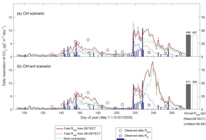
Soil CO2was in steady state (SS) during most of the
grow-ing season under the control soil texture (sandy clay loam) and precipitation conditions that assumed no antecedent af-fects (Ctrl scenario). For example, soil respiration (Rsoil)
predicted by the DETECT model was approximately equal toRsoil predicted by the SS-DETECT model during times
of no or little precipitation (Fig. 2a, days<218 or >230). Conversely,Rsoil predicted by the SS-DETECT model was
temporarily greater and more variable than that predicted by the DETECT model immediately following a large pre-cipitation event (Fig. 2a, days 218–229). However, the total cumulativeRsoil between days 92 to 274 – hereafter “total
growing seasonRsoil” – under SS (497 g C m−2)versus NSS
(498 g C m−2)assumptions was approximately equal (a dif-ference of∼0.2 %).
The differences between the Rsoil from DETECT and
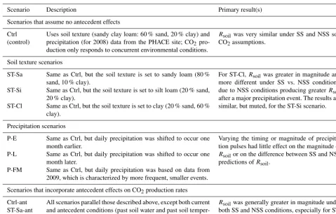
Table 3.The scenario code, description, and summary of results associated with each model scenario; the 14 scenarios below were applied to both the DETECT and SS-DETECT models. The scenarios involved a non-factorial combination of different soil texture, precipitation regimes, and inclusion/exclusion of antecedent effects on the root and microbial CO2production rates.
Scenario Description Primary result(s)
Scenarios that assume no antecedent effects
Ctrl (control)
Uses soil texture (sandy clay loam: 60 % sand, 20 % clay) and precipitation (for 2008) data from the PHACE site; CO2
pro-duction only responds to concurrent environmental conditions.
Rsoilwas very similar under SS and NSS soil
CO2assumptions.
Soil texture scenarios
ST-Sa Same as Ctrl, but the soil texture is set to sandy loam (80 %
sand, 10 % clay).
For ST-Cl,Rsoilwas greater in magnitude and
more different under SS vs. NSS conditions, due to NSS conditions producing greaterRsoil
after a major precipitation event. The results are similar, but muted, for the ST-Si scenario. ST-Si Same as Ctrl, but the soil texture is set to silt loam (20 % sand,
20 % clay).
ST-Cl Same as Ctrl, but the soil texture is set to clay (20 % sand, 60 % clay).
Precipitation scenarios
P-E Same as Ctrl, but daily precipitation was shifted to occur one
month earlier.
Varying the timing or magnitude of precipita-tion pulses had little effect on the magnitude of Rsoilor on the difference between SS and NSS
predictions ofRsoil.
P-L Same as Ctrl, but daily precipitation was shifted to occur one
month later.
P-FM Same as Ctrl, but daily precipitation was based on data from
2009, which is characterized by more frequent, smaller events.
Scenarios that incorporate antecedent effects on CO2production rates
Ctrl-ant ST-Sa-ant ST-Si-ant ST-Cl-ant P-E-ant P-L-ant P-FM-ant
All scenarios parallel those described above, except both current and antecedent conditions (past soil water and past soil temper-ature) are used in the calculation of the source terms (i.e., root and microbial CO2production rates).
Rsoilwas generally greater in magnitude under
both SS and NSS conditions, especially for Si-ant and Cl-ant (relative to Si and ST-Cl).
source terms of the models (Ctrl-ant scenario; Fig. 2b) were generally consistent with the results from the Ctrl sce-nario (Fig. 2a). However, the magnitude of Rsoil predicted
by both the DETECT and SS-DETECT models was up to 9 g C m−2day−1greater during days following the major rain event (i.e., during days 230–243) when antecedent condi-tions were considered. Moreover, the incorporation of an-tecedent effects led to a longer delay between the timing of the major rain event and the maximum Rsoil, which
oc-curred ∼five days later than when only current conditions were considered (Fig. 2a vs. 2b). As a result, total grow-ing season Rsoil was∼15 % higher under the Ctrl-ant
sce-nario (e.g., 571 g C m−2 under NSS assumptions, Fig. 2b) compared to the Ctrl scenario (e.g., 498 g C m−2under NSS, Fig. 2a). This increase in predictedRsoil under the Ctrl-ant
scenario for days 230–243 was primarily driven by greater root respiration (Fig. 2a vs. 2b).
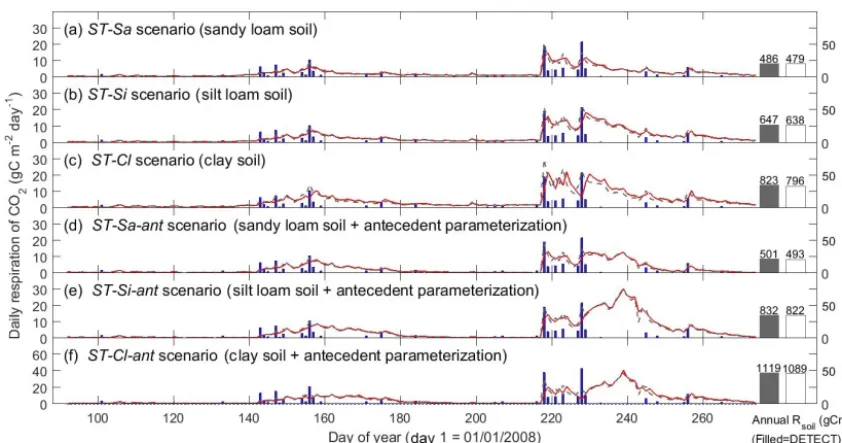
3.2 Effects of soil texture
Varying soil texture resulted in the greatest difference in daily Rsoil between the DETECT and SS-DETECT models;
how-ever, integrated over the growing season, these differences were very small (Fig. 3a, b, c). In particular, total grow-ing seasonRsoilpredicted by SS-DETECT was∼1.5 % less
than predicted by DETECT for soils consisting primarily of sand and silt (ST-Sa and ST-Si scenarios; Fig. 3a, b), but was∼3.3 % less for a clay dominated soil (ST-Cl scenario; Fig. 3c red versus grey bars). These differences inRsoilunder
NSS versus SS assumptions were approximately the same for the scenarios involving antecedent effects (Fig. 3d, e, f). Despite the minor differences at the growing season scale, notable differences emerged at the daily scale. For exam-ple, with the largest precipitation event of the year and the 10 days that followed (days 218–228), the median absolute difference between daily Rsoil from the SS-DETECT and
Figure 2.Time series of daily surface soil CO2fluxes (Rsoil)predicted by the non-steady-state (DETECT) and steady-state (SS-DETECT)
models over the growing season (1 April–30 September), based on the control scenarios(a)without (Ctrl) and(b)with (Ctrl-ant) antecedent effects (see Table 2). Only Rsoil is simulated using the SS-DETECT model, whereasRsoil and its root and microbial contributions are
simulated using the DETECT model. The predicted fluxes are overlaid with observed ecosystem respiration (Reco;Rsoil+aboveground
plant respiration) and microbial respiration (Rm; based on plots where vegetation was removed).
included (Figs. 3 and S3a, b). These differences increased to 31–35 % for the two clay soil texture scenarios (ST-Cl and ST-Cl-ant).
Soil texture also affected the magnitude of predictedRsoil
compared to the control scenarios, both with and without an-tecedent effects (Ctrl-ant and Ctrl, respectively). In particu-lar, we found that total growing season Rsoil, whether from
the DETECT or the SS-DETECT model, was ∼30 % and
∼60 % higher for the ST-Si and ST-Cl scenarios relative to the Ctrl scenario (Figs. 3b, c, 4a). The change inRsoil was
negligible, however, when the sand content was increased from 60 % (Ctrl) to 80 % (ST-Sa) for both models (Figs. 3a, 4a). The antecedent versions of the fine-textured scenarios (ST-Si-ant and ST-Cl-ant) resulted in ∼45 and ∼95 % in-creases in total growing seasonRsoil, respectively, compared
to the Ctrl-ant scenario (Figs. 3e, f, 4b). As with the Ctrl-ant scenario (Sect. 3.1), greater root respiration following the end of the second precipitation period between days 230 and 245, primarily drove the larger percentage increases for the SL-Si-ant and SL-Cl-SL-Si-ant scenarios compared to the non-SL-Si-antecedent versions.
3.3 Effects of precipitation regimes
Although varying the timing, frequency, or magnitude of pre-cipitation led to little difference betweenRsoil as predicted
by the DETECT and SS-DETECT models (Fig. S2), these precipitation regimes did affect the magnitude ofRsoil
pre-dicted by both models. For example, total growing season Rsoil predicted under the alternative precipitation scenarios
was lower relative to the Ctrl scenario. This decrease was relatively small (5–10 %) for the non-antecedent versions of the models (Fig. 4c), but was comparatively larger (15– 22 %) for the antecedent versions (Fig. 4d). This reduction appears to be driven by the amount of time over which daily Rsoil responded to the second precipitation period, which
occurred around day 220, 190, and 250 in the Ctrl, P-E, and P-L scenarios, respectively. Following this precipitation event, dailyRsoil achieved values around 10 g C m−2day−1
Figure 3.Time series of daily surface soil respiration (Rsoil)predicted from the non-steady-state (NSS) DETECT model (red solid lines)
and the steady-state (SS-DETECT) model (grey dashed lines), for different soil texture scenarios. The first three scenarios are the same as the control (Ctrl), except they assume a different soil texture:(a)more sandy soil,(b)more silty soil, or(c)more clayey soil. Panels(d),(e), and(f)show theRsoilpredictions from the same soil texture scenarios as in(a)–(c), but also include the antecedent effects of soil moisture
and temperature. See Table 2 for descriptions of each scenario.Rsoilpredictions are overlaid with daily precipitation.
Figure 4.Differences of total growing season (April–September) soil respiration (Rsoil)as predicted by the non-steady-state (DETECT) and
steady-state (SS-DETECT) models, for different pairs of scenarios. Comparisons are grouped so that they quantify the effects of(a)soil texture without antecedent effects,(b)soil texture with antecedent effects,(c)precipitation without antecedent effects,(d)precipitation with antecedent effects, and(e)antecedent effects. See Table 2 for descriptions of each scenario.
Ctrl scenario, which led to a reduction in total growing sea-sonRsoilin the P-FM scenario (Fig. S2c).
3.4 Effects of antecedent responses
When antecedent soil water content and soil temperature were included in the DETECT model we found that predicted Rsoilwas 15 % greater for the control scenario and 29–37 %
greater for the fine textured soil scenarios, compared to the corresponding scenarios that did not include antecedent
con-ditions (Fig. 4e). When the sand content was 80 % or for any of the different precipitation regimes, there was a negligible difference betweenRsoilpredicted by the antecedent versus
non-antecedent parametrizations of DETECT.
Daily Rsoil predicted by the DETECT model based on
the Ctrl and Ctrl-ant scenarios agreed well with observed ecosystem respiration (Reco), but Reco was slightly higher
than predictedRsoil (Fig. 2a, b), which was expected since Reco=Rsoil+aboveground autotrophic respiration. For the
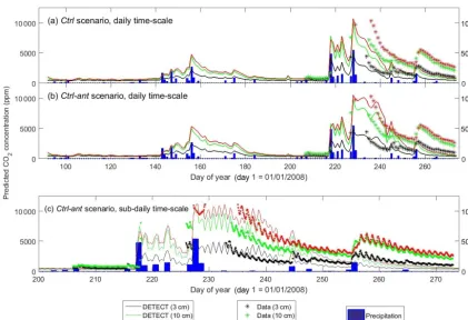
Figure 5.Time series of predicted versus observed soil CO2concentrations at 3 cm depth, 10 cm depth, and 20 cm depth, where the
pre-dictions are based on the non-steady-state (NSS) DETECT model. Predicted [CO2] is shown for the daily time scale for the control scenar-ios(a)without (Ctrl) and(b)with (Ctrl-ant) antecedent effects, and for(c)the subdaily (every 6 h) time scale for the Ctrl-ant scenario. Units are in parts per million (ppm).
the antecedent model terms were included (Fig. 2b) or not (Fig. 2a). Unfortunately,Recodata were not available during
the time period (days 230–250) associated with the greatest disagreement between the Ctrl and Ctrl-ant scenarios. During this period, frequent hourly measurements of soil [CO2] were
in better agreement with predicted soil CO2from the Ctrl-ant
scenario compared to the Ctrl scenario (Figs. 5a, b, S4a, b). After day ∼250, based on the DETECT model, both sce-narios (Ctrl and Ctrl-ant) under-predicted the observed soil [CO2] by∼50 % (Fig. 5).
4 Discussion
The DETECT and SS-DETECT models provide a framework for evaluating the circumstances under which steady-state (SS) assumptions of soil CO2production and surface soil
res-piration (Rsoil)are valid, and to identify the major physical
(i.e., soil texture, soil moisture) and/or biological (i.e., root and microbial respiration responses) factors that lead to non-steady-state (NSS) conditions.
4.1 Steady-state versus non-steady-state conditions
At the seasonal scale, there was reasonable agreement be-tween total growing seasonRsoilpredicted under the
assump-tion of SS versus NSS condiassump-tions, but the strength of this agreement depended on soil texture (see Sect. 4.2). At the daily scale,Rsoil predicted by the DETECT model deviated
from values expected under the assumption of SS conditions for 11 days or 4 % of the days during the April-September growing season (Fig. 2, days 218–228). These discrepan-cies, attributed to NSS conditions, were generally limited to periods following large rain events. For applications that assume SS conditions, such as isotopic partitioning studies (Hui and Luo, 2004; Ogle and Pendall, 2015), the SS as-sumption seemed reasonable during periods of minimal or no precipitation, representative of times during which soil water content changes very little or gradually. For sites or time pe-riods characterized by pulsed precipitation patterns, our re-sults suggested that NSS conditions would be more likely over longer periods of time.
4.2 Effect of varying soil texture
a predominantly (e.g., 60 %) sandy or silty soil, soil CO2
transport and efflux generally aligned with the SS assump-tion (Figs. 2, 3a–b). This was consistent with previous work that used SS models to predict Rsoil for similar soil types
(Baldocchi et al., 2006; Vargas et al., 2010).
For very fine-texture soil dominated by clay, however, SS assumptions were far less appropriate. The larger difference – relative to the Ctrl scenario – inRsoil predicted under SS
versus NSS conditions for fine-texture (i.e., 60 % clay) soil was apparent at both the growing season scale and the daily scale following a large precipitation event (Figs. 3, S3a, b). In general, the DETECT model predicted that Rsoil should
be higher in clay compared to sandy soil after precipitation events, a result supported by field experiments (Cable et al., 2008), but this texture effect is muted under assumptions of SS. Moreover, recovery ofRsoilto SS rates after a large rain
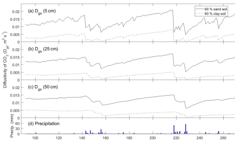
event took∼30 days in the clay soil (Fig. 3c, days 218 to 248) compared to∼10 days for the other coarser soil texture scenarios (Figs. 2, 3a–b, days 218 to∼230). These effects of soil texture on the prevalence of NSS conditions can be attributed to soil physical properties and their effects on air-filled porosity and CO2diffusivity. Fine textured soils have
smaller pores and tend to retain water for longer (Bouma and Bryla, 2000), which has the effect of decreasing soil CO2
diffusivity (Fig. 6). Thus, under moist conditions that follow a rain event, it may take about 15 min for a CO2 molecule
produced at 0.5 m to diffuse to the surface in a clay soil com-pared to only 1–2 min for a sandy soil. This means that the increase in CO2concentration near the soil’s surface will be
almost immediate under a coarsely textured soil (Fig. 6a), but slightly delayed under a finely texture soil. Finally, fine-textured soils have slower infiltration rates (Hillel, 1998), de-laying the exposure of more deeply distributed roots and mi-crobes to increased moisture availability. While this effect may not directly impact the SS assumption, it would lead to greater time lags between precipitation pulses and Rsoil
peaks.
These findings have important implications for studies that rely on the SS assumption to predict subsurface soil CO2
pro-duction. The SS assumption may be sufficient for systems defined by coarse-textured soils, but it may lead to erroneous conclusions if applied to fine-textured soils, especially at the very short-term scale (e.g., diurnalRsoil)during times of
pre-cipitation. Our simulation experiments made the simplifying assumption that soil texture is constant with depth, but in many ecosystems, texture may vary greatly with depth (Ogle et al., 2004). An important next step is to extend the simu-lations to explore the impacts of depth-varying soil texture on SS versus NSS conditions. The DETECT model can eas-ily accommodate such modifications; allowing soil texture to vary by depth would have a direct effect on soil water con-tent, which is simulated outside of DETECT using HYDRUS (Chou et al., 2008; Šim˚unek et al., 2008; Piao et al., 2009), and can accommodate such depth variation.
4.3 Effect of varying the timing or frequency of precipitation
Unlike soil texture, varying the timing, frequency, and mag-nitude of precipitation resulted in predictedRsoilthat was
al-most identical under SS and NSS assumptions, both at the growing season and daily time scales (Fig. S2). We had an-ticipated that such changes in the precipitation regime would impact SS conditions via impacts on soil air-filled porosity and potentially by changing the covariance between soil wa-ter and soil temperature, both of which affect soil CO2
dif-fusivity (e.g., see Eq. 2). We did not explore, however, the effect of decreasing the frequency while simultaneously in-creasing the magnitude of individual pulses. We hypothesize that this latter scenario could produce more exaggerated or extended NSS conditions given that large rain events would infiltrate deeper, reducing CO2diffusivity across greater soil
depths, thus slowing the transport of more deeply derived CO2. Increasing the number of small events, as done in the
P-FM scenario, would generally confine water inputs to shal-low layers, from which CO2has shorter distances to travel to
reach the surface, creating less opportunity forRsoil to
ex-hibit NSS behavior.
4.4 Effect of antecedent conditions
The inclusion or exclusion of antecedent soil moisture and temperature effects on CO2production rates had little to no
impact on the balance between SS versus NSS behavior of Rsoil. However, incorporating antecedent effects generally
increased the magnitude ofRsoil. This was for two reasons.
Firstly, microbial respiration was stimulated more during the initial onset of the main precipitation period when antecedent effects were considered (Fig. 2b vs. Fig. 2a, day 218, blue line). This is expected because the instantaneous response of microbes to a rain event is expected to be greater follow-ing a dry period compared to durfollow-ing a wet period (Xu et al., 2004; Sponseller, 2007; Cable et al., 2008, 2013; Thomas et al., 2008). These dynamics are incorporated in the an-tecedent version of the models when the parameter corre-sponding to the interaction between current and antecedent soil water content is negative (e.g.,α3, Table 1). Secondly,
root respiration was greatly enhanced following the end of this period of precipitation (Fig. 2b vs. Fig. 2a, days∼230– 250, green line), despite there being little precipitation after day 230 (Fig. 2b). This likely occurred because our DETECT model assumed that soil water over relatively longer time pe-riods (past 1–2 weeks, Eq. 12) affects current root respiration rates. This partly reflects the mechanism that roots are able to take up more soil water that has infiltrated to deeper depths (Cable et al., 2013). The microbes, however, are coupled to past conditions over comparatively short time periods (a cou-ple of days).
Figure 6.Time series of how the modeled diffusivity of CO2(Dgs)at three different depths (5, 25, and 50 cm) varies between a predominantly
sandy soil (solid line) and a predominantly clay soil (dashed line). Predictions are from the non-steady state (DETECT) model for the Ctrl (60 % sand) and ST-Cl (60 % clay) scenarios; see Table 2 for a description of the scenarios.
been well documented (Cable et al., 2013; Barron-Gafford et al., 2014; Ryan et al., 2015). Thus, we encourage future studies to include influences of past conditions when model-ing subsurface and surface CO2fluxes. Fortunately, our
sim-ulation experiments suggest that the lagged responses of mi-crobial and root respiration to soil moisture and temperature do not have a notable impact on the SS assumption.
4.5 Comparison of modeled soil CO2with data
The good agreement between modeled and observed soil CO2concentrations – particularly when including antecedent
effects – was very encouraging because the DETECT model was not rigorously tuned or calibrated to fit data on soil [CO2] or ecosystem CO2fluxes (Reco)(Figs. 5, S4a,b).
How-ever, discrepancies remained between the predicted and ob-served CO2fluxes, particularly after rain events. These
dis-crepancies could be an artifact of the input data used to cal-culate CO2production (i.e., the source term). Some
param-eter values were drawn from the literature and others were estimated by fitting a non-linear regression model to data. For example, the parameters describing the current and an-tecedent soil water content effects (α’s) were obtained by fitting a non-linear model to Reco data (Ryan et al., 2015).
While measuredRecorepresents both root respiration and
mi-crobial respiration contributions, it also reflects aboveground respiration, which is not currently treated in the DETECT model. Moreover, we made further assumptions about how the Reco parameter estimates translate to component
pro-cesses (root and microbial responses), and we relied on liter-ature information about how microbes and roots respond to precipitation events (e.g., the timing, magnitude, and lags). Future studies could rigorously fit the DETECT model to field data, such as observations ofRsoil, soil CO2
concentra-tions, and13C isotope fluxes. Using a Bayesian methodology to do this would allow one to incorporate multiple data sets to inform all parameters in DETECT.
4.6 Non-steady state model of soil CO2transport and production
An important contribution of this study was the development of a non-steady state (NSS) model of soil CO2 transport
and production (the DETECT model version 1.0), which is particularly useful for systems that may frequently experi-ence NSS conditions. Other comparable NSS models exist (e.g., Šim˚unek and Suarez, 1993; Fang and Moncrieff, 1999; Hui and Luo, 2004), but they generally treat the production (source) terms – root/rhizosphere respiration and microbial decomposition of soil organic matter – simplistically, and accompanying model code is not available. Our DETECT v1.0 model includes more detailed submodels for the produc-tion terms, inspired by recent studies (e.g., Lloyd and Tay-lor, 1994; Pendall et al., 2003; Davidson et al., 2012; Todd-Brown et al., 2012; Carrillo et al., 2014a); in contrast to these studies, which essentially described models for “bulk” soil, we applied the CO2 production models to every depth