On the use of the BMC to resolve Bayesian inference with nuisance parameters

R

A

On the use of the BMC to resolve Bayesian inference

with nuisance parameters

Edwin Privas*, Cyrille De Saint Jean, and Gilles Noguere

CEA, DEN, Cadarache, 13108 Saint Paul les Durance, France

Received: 31 October 2017 / Received infinal form: 23 January 2018 / Accepted: 7 June 2018

Abstract.Nuclear data are widely used in many researchfields. In particular, neutron-induced reaction cross sections play a major role in safety and criticality assessment of nuclear technology for existing power reactors and future nuclear systems as in Generation IV. Because both stochastic and deterministic codes are becoming very efficient and accurate with limited bias, nuclear data remain the main uncertainty sources. A worldwide effort is done to make improvement on nuclear data knowledge thanks to new experiments and new adjustment methods in the evaluation processes. This paper gives an overview of the evaluation processes used for nuclear data at CEA. After giving Bayesian inference and associated methods used in the CONRAD code [P. Archier et al., Nucl. Data Sheets118, 488 (2014)], a focus on systematic uncertainties will be given. This last can be deal by using marginalization methods during the analysis of differential measurements as well as integral experiments. They have to be taken into account properly in order to give well-estimated uncertainties on adjusted model parameters or multigroup cross sections. In order to give a reference method, a new stochastic approach is presented, enabling marginalization of nuisance parameters (background, normalization...). It can be seen as a validation tool, but also as a general framework that can be used with any given distribution. An analytic example based on afictitious experiment is presented to show the good ad-equations between the stochastic and deterministic methods. Advantages of such stochastic method are meanwhile moderated by the time required, limiting it’s application for large evaluation cases. Faster calculation can be foreseen with nuclear model implemented in the CONRAD code or using bias technique. The paper ends with perspectives about new problematic and time optimization.

1 Introduction

Nuclear data continue to play a key role, as well as numerical methods and the associated calculation schemes, in reactor design, fuel cycle management and safety calculations. Due to the intensive use of Monte-Carlo tools in order to reduce numerical biases, thefinal accuracy of neutronic calculations depends increasingly on the quality of nuclear data used. The knowledge of neutron induced cross section in the 0 eV and 20 MeV energy range is traduced by the uncertainty levels. This paper focuses on the neutron induced cross sections uncertainties evaluation. The latter is evaluated by using experimental data either microscopic or integral, and associated uncertainties. It is very common to take into account the statistical part of the uncertainty using the Bayesian inference. However, systematic uncertainties are not often taken into account either because of the lack of information from the experiment or the lack of description by the evaluators.

A first part presents the ingredients needed in the evaluation of nuclear data: theoretical models, microscopic and integral measurements. A second part is devoted to the presentation of a general mathematical framework related to Bayesian parameters estimations. Two approaches are then studied: a deterministic and analytic resolution of the Bayesian inference and a method using Monte-Carlo sampling. The next part deals with systematic uncertainties. More precisely, a new method has been developed to solve the Bayesian inference using only Monte-Carlo integration. A final part gives afictitious example on the235U total cross section and comparison between the different methods.

2 Nuclear data evaluation

2.1 Bayesian inference

Lety¼y~iði¼₁. . .NyÞ denote some experimentally mea-sured variables, and letxdenote the parameters defining the model used to simulate theoretically these variables andtis the associated calculated values to be compared with y. Using Bayes’theorem [1] and especially its generalization to * e-mail:[email protected]

©E. Privas et al., published byEDP Sciences, 2018

https://doi.org/10.1051/epjn/2018042 & Technologies

Available online at:

https://www.epj-n.org

continuous variables, one can obtain the well known relation between conditional probability density functions (writtenp

(.)) when the analysis of a new datasetyis performed:

pðxjy;UÞ ¼ pðxjUÞ⋅pðyjx;UÞ

∫dx⋅pðxjUÞ⋅pðyjx;UÞ; ð1Þ

whereUrepresents the“background”or“prior”information from which the prior knowledge of x is assumed. U is supposed independent of y. In this framework, the denominator is just a normalization constant.

The formal rule [2] used to take into account information coming from new analyzed experiments is:

posterior∝prior⋅likelihood: ð2Þ

The idea behind fitting procedures is to find an estimation of at least the first two moments of the posterior density probability of a set of parameters x, knowing an a priori information (or first guess) and a likelihood which gives the probability density function of observing a data set knowingx.

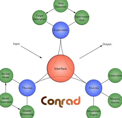
Algorithms described in this section are summarized and detailed description can be found in paper linked to the CONRAD code in which they are implemented [3]. A general overview of the evaluation process and the conrad code is given inFigures 1and2.

2.2 Deterministic theory

To obtain an equation to be solved, one has to make some assumptions on the prior probability distribution involved.

Given a covariance matrix and mean values, the choice of a multivariate joint normal for the probability densitypðxjUÞ

and for the likelihood is maximizing the entropy [4]. Adding Bayes’theorem, equation(1)can be written as follow:

pðxjy;UÞ∝e12½ðxxmÞTMx1ðxxmÞþðytÞTMy1ðytÞ; ð3Þ

where xm (expectation) and Mx (covariance matrix) are

prior information onx,yan experimental set and M_ythe associated covariance matrix.trepresents the theoretical model predictions.

The Laplace approximation is also made. It enables to approximate the posterior distribution by a multivariate normal distribution with the same maximum and curvature of the right side of equation(3). Then, it can be demonstrated that both the posterior expectation and the covariances can be calculated byfinding the minimum of the following cost function (Generalized Least Square):

x2GLS¼ ðxxmÞ T

M_x1ðxxmÞ þ ðytÞTM_y1ðytÞ: ð4Þ

To take into account non-linear effects and ensure a proper convergence of the algorithm, a Gauss–Newton iterative solution can be used [5].

Thus, from a mathematical point of view, the evaluation of parameters through a GLS procedure suffers from the Gaussian choice as guessed distribution for the

prior and the likelihood, the use of Laplace approximation, the linearization around the prior for Gauss-Newton algorithm and at last a 2nd order terms neglected in the Gauss–Newton iterative procedure.

2.3 Bayesian Monte-Carlo

Bayesian Monte-Carlo (BMC) methods are natural solutions for Bayesian inference problems. They avoid approximations and propose alternatives in probability

Fig. 1. General overview of the evaluation process.

density distribution choice for priors and likelihoods. This paper exposes the use of BMC in the whole energy range from thermal, resonance to continuum range.

BMC can be seen as a reference calculation tool to validate the GLS calculations and approximations. In addition, it allows to test probability density distributions effects and to find higher distribution moments with no approximations.

2.3.1 Classical Bayesian Monte-Carlo

The main idea of“classical”BMC is the use of Monte-Carlo techniques to calculate integrals. For any function f of random variable setx, any integral can be calculated by a Monte-Carlo sampling:

Z

pðxÞ⋅fðxÞdx¼lim

n∞! 1

n

Xn

k¼1

fðxkÞ !

; ð5Þ

wherep(x) is a probability density function. One can thus estimate any moments of the probability functionp(x). By definition, the mean value is given by:

〈x〉 ¼

Z

x⋅pðxÞdx: ð6Þ

Application of these simple features to Bayesian inference analysis gives for posterior distribution’s expectation values:

〈x〉 ¼ Z

x⋅Z pðxjUÞ⋅pðyjx;UÞ pðxjUÞ⋅pðyjx;UÞdx

dx: ð7Þ

The proposed algorithm to find out the first two moments of the posterior distribution is to sample the prior probability distribution functionpðxjUÞNx times and for eachxkrealization evaluate the likelihood:

Lk ¼pðykjxk;UÞ: ð8Þ

Finally, the posterior expectation and covariance is given by the following equation:

〈xi〉Nx ¼ XNx

k¼1

xi_;kLk

XNx

k¼1

Lk

; ð9Þ

〈xi;xj〉Nx¼ XNx

k¼1

xi_;k⋅xj_;k⋅Lk

XNx

k¼1

Lk

〈xi〉Nx〈xj〉Nx: ð10Þ

The choice of the prior distribution depends on what kind of analysis is done. If no prior information is given, a non-informative prior could be chosen (uniform distribu-tion). On the contrary, for an update of a given parameters set, the prior is related to a previous analysis with a known probability distribution function.

The use of Lk weights indicates clearly the major drawbacks of this classical BMC method: if the prior is far from high likelihood values and/or by natureLkvalues are small (because of the number of experimental points for example), then the algorithm will have difficulties to converge.

Thus, the main issue is that the covered phase space of sampling is not favorable to convergence. In practice a trial function close to the posterior distribution should be chosen for sampling.

More details can be found in paper [6].

2.3.2 Importance sampling

As previously exposed, the estimation of the integral off(x) times a probability density functionp(x) is not straightfor-ward. Especially in this Bayesian inference case, sampling the priorpðxjUÞdistribution, when it is far away from the posterior distribution or when the likelihood weights are difficult to evaluate properly, could be very expensive and time consuming without any valuable estimation of posterior distributions. The idea is then to sample in a different phase space region by respecting statistics.

This trial probability density function ptrial(x) can be

introduced by a trick as follow:

pðxÞ ¼ pðxÞ

ptrialðxÞ⋅ptrialðxÞ: ð11Þ

Thus, putting this expression in equation (5), one obtains the following equation:

Z

pðxÞ⋅fðxÞdx¼lim

n∞! 1

n

Xn

k_¼1

pðxkÞ

ptrialðxkÞ⋅fðxkÞ !

: ð12Þ

Then, sampling is done on the trial probability density function ptrial(x) getting a new set of {xk}. For each

realizationxk, an evaluation of additional terms

p_ðxÞ pbiasðxÞ

is necessary.

As a result, expectation and covariances are defined by:

〈xi〉Nx ¼ XNx

k¼1

xi;k⋅hðxkÞ⋅Lk

XNx

k_¼1

hðxkÞ⋅Lk

; ð13Þ

and

〈xi;xj〉Nx ¼ XNx

k¼1

xi;k⋅xj;k⋅hðxkÞ⋅Lk

XNx

k_¼1

hðxkÞ⋅Lk

〈xi〉Nx〈xj〉Nx; ð14Þ

withhðxkÞ ¼ pðxkjUÞ

p_trialðxkÞ.

The choice of trial functions is crucial and the closer to the true solutionptrial(x) is, the quicker the algorithm

comes from the result of the generalized least square (with additional standard deviation enhancement). Many other solutions can be used depending on the problem.

3 Systematic uncertainties treatment

3.1 Theory

Let recall some definitions and principles. First, it is possible to link model parameters x and nuisance parametersuwith conditional probability:

pðx;ujy;UÞ ¼pðxju;y;UÞ⋅pðujy;UÞ; ð15Þ

withUthe prior information on both model and nuisance parameters. The latter is supposed independent to the measurement. It means nuisance parameters are consid-ered acting on experimental model. It induces

pðujy;UÞ ¼pðujUÞ;giving the following equation:

pðx;ujy;UÞ ¼pðxju;y;UÞ⋅pðujUÞ: ð16Þ

Moreover, evaluators are looking at the marginal probability densitypðx;ujy;UÞ;also written p_uðxjy;UÞ. It is given by the integration of the probability density function over marginal variables as follow:

p_uðxjy;UÞ ¼ Z

pðx;ujy;UÞdu: ð17Þ

According to(16), the follow equation is obtained:

p_uðxjy;UÞ ¼ Z

pðxju;y;UÞ⋅pðujUÞdu: ð18Þ

Then the Bayes theorem is used to calculate the first integral term of(18):

pðxju;y;UÞ ¼Z pðxjUÞ⋅pðyju;x;UÞ pðxjUÞ⋅pðyju;x;UÞdx

: ð19Þ

This expression is right if both model and nuisance parameters are supposed independent. According to(18) and(19), the marginal probability density function of the a posteriori model parameters is given by:

p_uðxjy;UÞ ¼ Z

pðujUÞduZ pðxjUÞ⋅pðyju;x;UÞ pðxjUÞ⋅pðyju;x;UÞdx

: ð20Þ

3.2 Deterministic resolution

The deterministic resolution is well described in Habert thesis [7]. Several works have beenfirst performed in 1972 by H. Mitani and H. Kuroi [8,9] and later by Gandini [10] giving a formalism to the multigroup adjustment and a way to take into account the systematic uncertainties. These were the first attempts to consider the possible

presence of systematic errors in a data adjustment process. Equations are not detailed here, only the idea and the final equation is provided.

Let Mstat_x be the a posteriori covariance matrix obtained after an adjustment. The a posteriori covariance after marginalization Mmarg_x can be found as follow:

Mmarg_x ¼Mstat_x þ ðG_xTGxÞ1⋅GTx⋅GuMuGTu⋅Gx⋅ðGTxGxÞ1 ð21Þ

withGxsensitivities vector of the calculated model values

to the model parameters andG_usensitivities vector of the calculated model values to the nuisance parameters. Similar expressions have been given in reference [8,9] where two terms appear: one for classical resolution and the second for some added systematic uncertainties.ðGT_xGxÞis a square matrix supposed reversal. It is often the case when there are more experimental points than fitted parameters. If numeric issues appeared, it is mandatory to find another way, giving by a stochastic approach. Further study should be undertaken to compare the deterministic method proposed here and the one identified in Mitani’s papers in order to provide a more robust approach.

3.3 Semi-stochastic resolution

This method (written MC_Margi) is easy to understand starting from the equation (20): nuisance parameters are sampled according to a Gaussian distribution and for each history, a deterministic resolution is done (GLS). At the end of every simulation, parameters and covariances are stored. When all the histories have been simulated, the covariance total theorem gives thefinal model parameters covariance. The methods is not developed here but more detailed can be found in papers [7,11].

3.4 BMC with systematic treatment

BMC method can deal with marginal parameters without deterministic approach. This work has been successfully implemented in the CONRAD code. One wants tofind the posterior marginal probability function defined in equation (20). It is similar to the case with no nuisance parameters but with two integrals. Same weighting principle can be applied by replacing the likelihood term by a new weightw_uðxjyÞdefined by:

w_uðxjyÞ ¼ Z

pðujUÞ⋅pðyju;x;UÞ Z

pðxjUÞ⋅pðyju;x;UÞdx

du: ð22Þ

The very close similarities between the case with no marginal parameter enabled a quick implementation and understanding. Finally, the previous equation gives:

Both integrals can be solved using a Monte-Carlo approach. The integral calculation of the equation(22)is done as follow:

w_uðxjyÞ ¼ _lim

n_u→∞ 1

n_u Xn_u

l¼0

pðyjul;x;UÞ Z

pðxjUÞ⋅pðyjul;x;UÞdx 0 B B @ 1 C C

A: ð24Þ

Then_uhistories are calculated by sampling according to

pðujUÞ. The denominator’s integral of equation(24)is then computed:

∀l∈⟦1;n_u⟧; Z

pðxjUÞ⋅pðyjul;x;UÞdx¼ _lim

nx→∞

1

nx

Xnx

m¼0

pðyjul;xm;UÞ !

:

ð25Þ

Thenxhistories are evaluated by sampling according to pðxjUÞ. Mixing equations(24) and (25), the new weight

w_uðxjyÞis given by:

lim n_u→∞

1

n_u Xn_u

l_¼0

pðyjul;x;UÞ

lim nx→∞

1

nx

Xnx

m_¼0

pðyjul;xm;UÞ ! 0 B B B B @ 1 C C C C

A: ð26Þ

Let us consider Nx is the number of history sampled

according the prior parameters and N_u is the number of history sampled according the marginal parameters. The larger those number are, the more converge the results will be. The previous equation can be numerically written with no limits as follow:

w_uðxjyÞ ¼Nx N_u

XN_u

l¼0

pðyjul;x;UÞ XNx

m¼0

pðyjul;xm;UÞ

: ð27Þ

In order to simplify the algorithm, N_u and Nx are

considered equal (introducing N asN=N_u=Nx). First, N

samples are drawn according toukand xk. Equation(26)

can be simplified as follow:

w_uðxjyÞ ¼X

N

l¼0

pðyjul;x;UÞ

XN

m¼0

pðyjul;xm;UÞ

: ð28Þ

In CONRAD, the N*N values of the likelihood are stored (i.e. ∀ði;jÞ∈⟦1;N⟧2;pðyj_uj;xi;UÞ. Those values are required to perform statistical analysis at the end of the simulation. The weight for an history k is then calculated:

w_uðxkjykÞ ¼X

N

l¼0

pðykjul;xk;UÞ

XN

m¼0

pðykjul;xm;UÞ

: ð29Þ

To get the posterior mean values and the posterior correlation, one should apply the statistical definition and get the two next equations:

〈x〉N ¼ 1

N

XN

k¼0

xk⋅

XN

l¼0

pðyjul;xk;UÞ

XN

m¼0

pðyjul;xm;UÞ

; ð30Þ

Covðxi;xjÞN ¼ ðMxpostÞ

Nx

ij

¼ 〈xixj〉N 〈xi〉N〈xj〉N; ð31Þ

with 〈xixj〉N defined as the weighting mean of the two parameters product:

〈xixj〉N ¼ 1

N

XN

k_¼1

xi_;k⋅xj_;k⋅w_uðxkjykÞ: ð32Þ

4 Illustrative analysis on

U total cross

section

4.1 Study case

The selected study case is just an illustrative example giving a very first step towards the validation of the method, its applicability and potential limitations. The 238_{U total cross section is chosen and fitted on the}

unresolved resonance range, between 25 and 175 keV. The theoretical cross section is calculated using the R mean matrix model. The main sensitives parameters in this energy range is the twofirst strength functionsSl= 0and

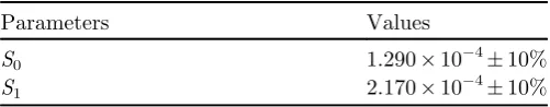
Sl= 1. Tables 1 and 2 give respectively the spin confi g-urations and the prior parameters governing the total cross section. An initial relative uncertainties of 15% is taken into account with no correlations. The experimental dataset used comes from the EXFOR database [12]. A 1% arbitrary statistical uncertainty is chosen.

Table 1. 238

U spin configuration considered for resonance wavessand p.

l s Jp gJ onde

238_{U (0}+_{) 0 1/2 1/2}+ _{1 s}

1 1/2 1/2 3/2 1 2 p

Table 2. Initial URR parameters with no correlation.

Parameters Values

S0 1.290104± 10%

4.2 Classical resolution with no marginal parameters

All the methods have been used to perform the adjustment. One million histories haven been simulated in order to get the statistical values converged below 0.1% for the mean values and 0.4% for the posterior correlation. The convergence is driven by how far the solution is from the prior values. Table 3shows the overall good results coherence. Very small discrepancies can be seen for the classical methods caused by

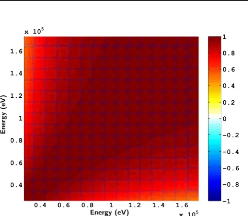
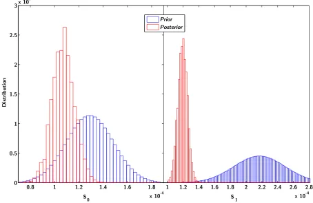
the convergence issues. For a similar number of history, the importance methods converged better than the classical BMC. The prior covariance on the total cross section is given onFigure 3. The anti-correlation created betweenS0andS1 directly give correlations between the low energy and the high energy (seeFig. 4). The prior and posterior distribution engaged in the BMC methods are given inFigure 5. One can notice the Gaussian distributions for all the parameters (both prior and posterior).

Table 3. Results comparison between the different methods implemented in CONRAD for238U total cross section.

Physical quantities Prior GLS BMC Importance

S0(104) 1.290 1.073 1.072 1.073

dS0(106) 19.35 9.013 9.122 9.020

S1(104) 2.170 1.192 1.193 1.192

dS1(106) 32.55 6.089 6.135 6.095

Correlation 0.000 0.446 0.425 0.447

x2 381.6 8.78 8.79 8.78

〈dyi(%) 2.78 0.64 0.65 0.64

Fig. 3. A priori covariance matrix on238_{U total cross section.}

Table 4. Results comparison when a normalisation marginal parameter is taken into account. AN_Margi represents the deterministic method, MC_Margi represents the semi-stochastic resolution, BMC is the classical method and the last column called Importance is the BMC where an importance function is used for the sampling.

Physical quantities AN MC_Margi BMC Importance

S0(10 4

) 1.073 1.073 1.063 1.074

dS0(106) 9.634 9.469 8.939 9.490

S1(104) 1.192 1.194 1.215 1.193

dS1(106) 11.60 11.52 8.945 11.54

Correlation 0.081 0.035 0.061 0.044

〈dyi(%) 1.19 1.17 0.93 1.18

4.3 Using marginalization methods

This case is very closed to the previous paragraph. But this time, a nuisance parameter is taken into account. More precisely, a normalization is considered with a systematic uncertainties of 1%. 10 000 histories are sampled for the MC_Margi case (semi-stochastic resolution) and 10 00010 000 for BMC methods. For the importance resolution, the biasing function is the posterior solution coming from the deterministic resolution. All the results seem to be equivalent, as shown inTable 4. However, the classical BMC is not fully converged because slight

differences are found between the means values.Figures 6 and 7 show the mean values convergence using the stochastic resolutions, showing one more time not converged results with the classical BMC method. Calculation time are longer with marginal parameters. This is explained by the method which the idea is to perform a double Monte-Carlo integration. The good coherence on the mean values and correlation between parameters give identical posterior correlation on the total cross section.Figure 8 shows the a posteriori covariance, whatever methods chosen.

Fig. 5. S0andS1distributions obtained with the classical BMC method.

5 Conclusions

The use of BMC methods was exposed in this paper and an illustrative analysis was detailed. One important point is that these methods could be used for resonance range analysis (both resolved and unresolved resonance) as well as higher energy models. In addition, both microscopic and integral data assimilation could be achieved. Nevertheless, the major issue is related to the convergence estimator: depending on which parameters are investigated (central values or correlation between them), the number of histories (sampling) could be very different. Indeed, special care should be taken for the correlations calculation because an additional order of magnitude of sampling histories could be necessary. Furthermore, it was shown that sampling priors are not a problem. It is more efficient to properly sample in the phase space region where the likelihood is large. In this aspect, Importance and Metropolis algorithms are working better than brute force (“classical”) Monte-Carlo. It also highlights the fact that pre-sampling prior with a limited number of realizations could be inadequate for further inference analysis. The integral data assimilation with feedback directly on the model parameter is too much time consuming. However, a simplified model can be adopted by using a simple model with a linear approach for instance (to predict integral parameters response to input parameters). Such approxi-mation would be less consuming but will erase non-linearity effect that may be observed in the posterior distribution. Such study should be performed with extensive cases to improve the Monte-Carlo methods.

Concerning BMC inference methods, in the future, other Markov chain algorithms will be developed in CONRAD code and efficient convergence estimators will be proposed as well. The choice of Gaussian probability functions for both prior and likelihood will be challenged and discussed.

More generally, an open range of scientific activities will be investigated. In particular, one major issue is related to a change in paradigm: to go beyond covariance matrices and deal with parameters knowledge taking into account full probability density distributions. In addition, for end-up users, it will be necessary to investigate the feasibility of a full Monte-Carlo approach, from nuclear reaction models to nuclear reactors or integral experiments (or any other applications) without format/files/processing issues which are most of the time bottlenecks.

The use of Monte-Carlo could solve a generic issue in nuclear data evaluation related to difference of information given in evaluatedfiles: in the resonance range where cross section uncertainties and/or nuclear model parameters uncertainties are compiled and in the higher energy range where only cross section uncertainties are formatted. This could simplify the evaluation of full covariance over the whole energy range.

Author contribution statement

The main author (E. Privas) has done the development and the analysis of the new stochastic method. The other authors participated in the verification process and in the overall development of CONRAD.

References

1. T. Bayes, Philos. Trans. R. Soc. London53, 370 (1763) 2. F. Frohner, JEFF Report 18, 2000

3. P. Archier, C. De Saint Jean, O. Litaize, G. Noguère, L. Berge, E. Privas, P. Tamagno, Nucl. Data Sheets118, 488 (2014) 4. T. Cover, J. Thomas,Elements of information theory

(Wiley-Interscience, New York, 2006)

5. R. Fletcher,Practical methods of optimization(John Wiley & Sons, New York, 1987)

6. P.A.C. De Saint Jean, E. Privas, G. Noguère, inProceeding of the International Conference on Nuclear Data,2016

7. B. Habert, Ph.D. thesis, Institut Polytechnique de Grenoble, 2009

8. H. Mitani, H. Kuroi, J. Nucl. Sci. Technol.9, 383 (1972) 9. H. Mitani, H. Kuroi, J. Nucl. Sci. Technol.9, 642 (1972) 10. A. Gandini, Y. Ronen Ed.Uncertainty analysis(CRC Press,

Boca Raton, 1988)

11. C. De Saint Jean, P. Archier, E. Privas, G. Noguère, O. Litaize, P. Leconte, Nucl. Data Sheets123, 178 (2015)

12. C. Uttley, C. Newstead, K. Diment, in Nuclear Data For Reactors, in ConferenceProceedings(Paris, 1966), Vol.1, p. 165

Cite this article as: Edwin Privas, Cyrille De Saint Jean, Gilles Noguere, On the use of the BMC to resolve Bayesian inference with nuisance parameters, EPJ Nuclear Sci. Technol.4, 36 (2018)